仿效兔子視網膜開持續中樞神經細胞之視覺神經晶片

全文

(1)國立交通大學電子工程學系電子研究所碩士論文仿效兔子視網膜開持續中樞神經細胞之視覺神經晶片 A NEUROMORPHIC CHIP THAT IMITATES THE ON SLUGGISH SUSTAIN GANGLION CELL SET IN THE RETINA OF RABBITS. 研究生：許筱妊指導教授：吳重雨教授. 中華民國九十七年八月.

(2) 仿效兔子視網膜開持續中樞神經細胞之視覺神經晶片. A NEUROMORPHIC CHIP THAT IMITATES THE ON SLUGGISH SUSTAIN GANGLION CELL SET IN THE RETINA OF RABBITS. 研究生：許筱妊. Student: Xie-Ren Hsu. 指導教授：吳重雨教授. Advisor: Chung-Yu Wu. 國立交通大學. 電子工程學系電子研究所碩士班碩士論文 A Thesis Submitted to Institute of Electronics College of Electrical Engineering and Computer Science National Chiao Tung University in partial Fulfillment of the Requirements for the Degree of Master in Electronic Engineering August 2008 Hsin-Chu, Taiwan, Republic of China. 中華民國九十七年八月.

(3) 仿效兔子視網膜開持續中樞神經細胞之視覺神經晶片仿效兔子視網膜開持續中樞神經細胞之視覺神經晶片. 研究生：研究生：許筱妊. 指導教授：指導教授：吳重雨老師. 國立交通大學電子工程學電子工程學系. 電子研究所碩士班電子研究所碩士班. 摘要哺乳類動物視網膜由五種不同的細胞構成，而每一種細胞又各自有不同的分類與功能。除了將影像世界的訊息轉變為神經訊號外，視網膜還負責 0.3%的大腦視覺處理功能。在本研究中，我們嘗試以工程的角度去瞭解視網膜的運作功能。於本論文中，我們提出了一個新的設計方法用以設計金氧半場效電晶體神經型態晶片，此神經型態晶片依據由哺乳類動物視網膜建立之生物模型所設計的仿視網膜矽晶片，模擬了兔子視網膜的開持續中樞神經節細胞組；文中詳論其特性與工作原理。此晶片包含一個大小為 32x32 的影像感測陣列，可仿效兔子視網膜開持續中樞神經細胞的功能。陣列中包含了許多相同的基本單元，而每個基本單元中包含了光輸入元件、感光細胞、水平細胞、開兩極細胞、關兩極細胞、Amacrine 細胞與中樞神經細胞元件。晶片中還包括了輸入輸出接墊（I/O pads）的靜電防護、位址解碼（address decoder）及訊號讀出電路。最後，我們比較原本生物模型的結果與電路模擬及晶片的量測結果之異同，檢驗此晶片的正確性與待改進之處。量測結果顯示，該金氧半場效電晶體神經型態晶片在時域及空間域的特性與生物量測結果相符，驗證了該晶片的仿生功能。經由實驗驗證，這個設計方法所設計的神經型態晶片能協助尚未揭露的視網膜細胞行為與視覺語言，並且也可用以設計所有的視網膜神經節細胞組，將視網膜功能完全由晶片實現。此外，該研究結果也使得極具潛力的視網膜晶片應用，諸如運動偵測、電腦視覺、人工視網膜和生醫元件方面變的更有可行性。 i.

(4) A NEUROMORPHIC CHIP THAT IMITATES THE ON SLUGGISH SUSTAIN GANGLION CELL SET IN THE RETINA OF RABBITS. Student: Xie-Ren Hsu. Advisor: Chung-Yu Wu. Department of Electronics Engineering & Institute of Electronics National Chiao Tung University. ABSTRACT The mammalian retina is comprised of five different kinds of cells, for each kind can be divided into more types. Besides transducing the visual world into neural signals, these cells are in charge of 0.3% of the visual function of the brain. In this research, we try to understand the retinal functions from the engineering point of view. In this thesis, a new design methodology is proposed to implement CMOS neuromorphic chips which imitate the ON sluggish sustain ganglion cell set of rabbits’ retinas. A retinal chip based on the biological model derived from the mammalian retina is proposed. The retinal chip contains a focal plane sensory array of 32x32 similar basic cells that perform the functions. Each basic cell contains photo-input, photoreceptor, horizontal cell, on bipolar cell, off bipolar cell, amacrine cell and ganglion cell. ESD protection circuit for I/O pads, address decoders and readout circuits are also included in this chip. Finally, the results of HSPICE simulation and chip measurement are compared with that of the original model to examine the consistency and the difference for further improvement. The ii.

(5) measurement results on the fabricated CMOS neuromorphic chip are consistent with the biological measurement results. Thus the biological functions of the chip have been successfully verified. It can be used to understand more biological behaviors and visual language of retina under different input optical images which have not yet been tested in biological experiments. Based on the results, the full ganglion cell sets of retina can be designed. Otherwise, many potential applications of retinal chips on motion sensors, computer vision, retinal prosthesis, and biomedical devices are feasible.. iii.

(6) ACKNOWLEDGEMENT 感謝指導教授吳重雨博士，給予我能夠受到這個環境薰陶的機會。ㄧ年半來耐心的指導與鼓勵，使我能順利完成碩士學位。在吳教授循序漸進的諄諄教誨下，前瞻的見解與淵博的專業知識，給予我指導與啟發，讓我不僅獲得許多積體電路設計的專業知識，更學習到研究時應有的挑戰困難及解決問題的態度與方法，面對問題時如何著手構思和勇於嘗試，使我得以一點一滴地累積自己的實力，雖然在過程倍感艱辛，但卻獲益良多。此外，我要特別感謝林俐如教授和楊文嘉學長，在研究上所給予的教導與協助，並給予我寶貴的建議與指導，真的很感謝你們。祝福你們研究順利、事事順心，也祝福學長早日畢業。感謝307實驗室的王文傑學長、虞繼堯學長、陳勝豪學長、黃祖德學長、盧台祐學長、黃鈞正學長、蘇烜毅學長、蔡夙勇學長、陳旻珓學長在研究上所給予的指導與協助，給予我指點和研究上的經驗傳承。同時也感謝所有碩班的學長姐與同學。感謝國忠、順哥、萬諶、維德、豪哥、松諭、巧玲、威宇、建名、期聖、國權、政邦、亭州、區文、世範、宗恩、紹岐、柏硯、歐陽、昕華、國維、晟佑等學長姐的諸多幫助。還要謝謝惠雯、佳琪、怡歆、家菱、炯為、宗昀、韋丞、順天、暄泰、彥良、哲倫、世昕、凱悌、彥瑋、育祥、詠儒以及所有新進來的學弟妹們一起奮鬥玩樂所建立那起無堅不摧的友誼情感，在生活上所帶來的歡樂與相互幫忙。謝謝你們一直以來的陪伴與關懷。此外，特別感謝當初帶我進入電路設計領域的大學專題教授：翁若敏博士。感謝老師的啟蒙與教導，平日的叮嚀與教誨，一直以來的提攜與指引、支持與鼓勵，讓我得以在電路設計領域紮下穩固的基礎進而深入研究。如師亦友的相處，也為冷浚的生涯平添華麗且優美樂章！更教導了人生旅途上遇到的挫折該如何面對，使得我在專業知識增長的同時，更學習到為人處世的珍貴態度。在此獻上最誠懇的謝意。最後感謝我的父親許清堃先生、母親張淑媛女士，感謝你們無怨無悔、永無止境的付出、照顧、支持與鼓勵，給予我最溫暖的關心，你們是我學習過程中最大的後盾，衷心的感謝你們。在此，僅以這份小小的成果與你們分享，並致上深深的感謝之意。謹以此論文獻給所有關心我的人，並祝福我的師長、家人、朋友及學弟妹們事事順心、身體健康。我在撰寫的過程中，雖力求嚴謹，然誤謬之處，在所難免，尚祈各位讀者賜予寶貴意見，使本論文能更加完善。. 許筱妊誌於風城交大九十七年盛夏 iv.

(7) CONTENTS ABSTRACT (CHINESE)……………………………………….….….….i ABSTRACT (ENGLISH)……………………………………….……..…ii ACKNOWLEDGEMENT…………………………..……...………..…..iv CONTENTS………………………………………………………........….v TABLE CAPTIONS……………………………………………….....…vii FIGURE CAPTIONS……………………………………………....…..viii. CHAPTER 1 1.1. Introduction.…………………………………………………..…...……1. BACKGROUND……………………………………………………………………...…...1 1.1.1. Morphology and physiology of retina……………………………….…………1. 1.1.2. The classification of ganglion cells of the rabbits’ retina…………………..4. 1.2. OPERATIONAL PRINCIPLE – FROM THE ENGINEERING POINTS OF VIEW………….5. 1.3. MOTIVATIONS…………………………………………………………………………...8. 1.4. MAIN RESULTS………………………………………..………………………………...9. 1.5. THESIS ORGANIZATION………………………………………………………………..10. CHAPTER 2. The CNN Model of the ON Sluggish Sustain Ganglion Cell.............................................................................................................15. 2.1. NEUROMORPHIC MODEL OF THE RETINAL CELL SET…………………….…..….....15. 2.2. MACROMODEL FOR CHIP IMPLEMENTATION……………………….……………….17 v.

(8) 2.3. SIMULATION RESULTS…………………….……………………………….…………..18. CHAPTER 3. Circuit Design…………………………………………….……...…..26. 3.1. ARCHITECTURE OF A BASIC CELL OF THE RETINAL CHIP…………………..…...…26. 3.2. CIRCUIT DESIGN OF THE BASIC CELL…………………..…………………….………27 3.2.1 Photoreceptor and Horizontal cell………..…………………….……….……27 3.2.2 On bipolar cell………..…………………………………………………...……...28 3.2.3 Off bipolar cell………..…………………….……………………………..……...29 3.2.4 Amacrine and Ganglion cells………..……………………………….….……..34 3.2.5 Impacts of device leakage and mismatch………..………………...….…..….34. 3.3. ARCHITECTURE OF 2-D RETINAL ARRAY…..………………...…….……..…..……...35. 3.4. SIMULATION RESULTS…..………………...…….……..………………...…….....……35. CHAPTER 4. Layout Descriptions and Experimental Results….…....53. 4.1. LAYOUT DESCRIPTIONS……………………………………………………………….53. 4.2. EXPERIMENTAL ENVIRONMENT…………………………………………......…….…54. 4.3. EXPERIMENTAL RESULTS………………………………………………………..….…55. CHAPTER 5. Conclusions and Future Work…………………………..…….72. 5.1. CONCLUSIONS…….……………………………………………………………….…….72. 5.2. FUTURE WORK…….……………………………………………………………....….….73. REFERENCES..........................................................................................................................74. vi.

(9) TABLE CAPTIONS. CHAPTER 1 Table I. Ganglion cell types, defined by response to spot sizes and level of dendritic stratification [13]……………………………………………………………………….11. CHAPTER 3 Table II. The transistor’s sizes of circuits in Fig. 3. 2(a)-(d)…………………………………….39. CHAPTER 4 Table III. The bias condition to measure the spatiotemporal patterns of Fig. 4. 7………………..58. Table IV. Summary of characteristics of the proposed 32x32 retinal chip………………………..69. vii.

(10) FIGURE CAPTIONS CHAPTER 1 Fig. 1.1. Schematic of the mammalian retina. Reprinted from [1]………………………………..12. Fig. 1.2. The major cell types of a typical mammalian retina. From the top row to the bottom, photoreceptors, amacrine cells and ganglion cells. Reprinted from [2]………………….12. Fig. 1.3. Bipolar cell types of the primate retina. Reprinted from [1]……………………………..13. Fig. 1.4. Spiking patterns in each row (measured from four different members of the same cell class) for five different classes of ganglion cells. The numbers at the beginning of each row refer to the classification shown in Table 1. 1. The arrows in row 5 (cell type 7) point to the enhanced activity at the stimulus edge, a feature that is characteristic of this class [13]……………………………………………………………………………………….13. Fig. 1.5. A sketch of the processing structure of the CNN model of the mammalian rabbit retina [14]……………………………………………………………………………………….14. CHAPTER 2 Fig. 2.1. The neuromorphic model of the ON sluggish sustain ganglion cell set of rabbits’ retinas. The parameter τ denotes the time constant in millisecond of the LPF. The parameter D denotes the space constant, which is defined by the laterally diffusing range in cell number in a 180-cell array………………………………………………………………..21. Fig. 2.2. The RC equivalent model of the ON sluggish sustain ganglion cell set of rabbits’ retinas…………………………………………………………………………………….21. viii.

(11) Fig. 2.3. The macromodel of a single pixel of the implemented chip…………………………….22. Fig. 2.4. The HSPICE model-simulated time domain waveforms of the neuromorphic model of the ON sluggish sustain cell set in a 32x32 array for (a) photoreceptor, (b) horizontal cell, (c) ON bipolar cell, (d) OFF bipolar cell, (e) amacrine cell, and (f) ganglion cell. These waveforms are recorded from the 17th row of the array. The x-axis is normalized time and the y-axis is the pixel location which denotes space. The stimulus is applied to the 15th to the 20th pixel at time point 1001 to 2000………………………………………………...23. Fig. 2.5. The HSPICE model-simulated space domain waveforms of the neuromorphic model of the ON sluggish sustain cell set in a 32x32 array for (a) photoreceptor, (b) horizontal cell, (c) ON bipolar cell, (d) OFF bipolar cell, (e) amacrine cell, and (f) ganglion cell. These waveforms are recorded from the 17th row of the array. The x-axis is normalized time and the y-axis is the pixel location which denotes space. The stimulus is applied to the 15th to the 20th pixel at time point 1001 to 2000………………………………………………...24. Fig. 2.6. The HSPICE model-simulated time domain waveforms of the neuromorphic model of the ON sluggish sustain cell set in a 32x32 array for (a) photoreceptor, (b) horizontal cell, (c) ON bipolar cell, (d) OFF bipolar cell, (e) amacrine cell, and (f) ganglion cell. These waveforms are recorded from the 17th row of the array. The x-axis is normalized time and the y-axis is the pixel location which denotes space. The stimulus is applied to the 15th to the 20th pixel at time point 1001 to 2000. The waveform at the left of each pattern is the spatial domain waveform(s) obtained at the time marked by the vertical arrow(s). The waveform at the bottom of each pattern is the temporal domain waveform obtained at the location marked by the horizontal arrow. The Vsm = 2.2V……………………………….25. ix.

(12) CHAPTER 3 Fig. 3.1. The block diagram of a single pixel……………………………………………………...40. Fig. 3.2. (a) The circuit of the photoreceptor and horizontal cell (PH1, PH2, H); (b) The circuit of ON bipolar cell (ONBIP); (c)OFF bipolar cell (OFFBIP); (d) The circuit of amacrine and ganglion cells (Ama, GC)………………………………………………………………...43. Fig. 3.3. (a) A linearized transconductor using floating voltages sources; (b) Flipped Voltage Follower implementation; (d) Transconductor using two identical FVFs to implement the floating batteries.………………………………………………………………………....44. Fig. 3.4. (a) The whole chip architecture of the implemented chip, and (b) the implementation of smoothing networks……………………………………………………………………...45. Fig. 3.5. The schematic of the address decoder used in the chip (a) column address decoder; (b) row address decoder; (c) buffer; (d)AND gate…………………………………………...48. Fig. 3.6. The monte carlo analysis of OFF bipolar cell with (a) the original V-I converter structure (b) the modified linear transconductor structure.…………………….…………………..49. Fig. 3.7. The HSPICE circuit-simulated time domain waveforms of the neuromorphic model of the ON sluggish sustain cell set in a 32x32 array for (a) photoreceptor, (b) horizontal cell, (c) ON bipolar cell, (d) OFF bipolar cell, (e) amacrine cell, and (f) ganglion cell. The light stimulus is applied at 1000th~2000th micro-second and Vsm = 2.2V……………………..50. Fig. 3.8. The HSPICE circuit-simulated space domain waveforms of the neuromorphic model of the ON sluggish sustain cell set in a 32x32 array for (a) photoreceptor, (b) horizontal cell, (c) ON bipolar cell, (d) OFF bipolar cell, (e) amacrine cell, and (f) ganglion cell. The light stimulus is applied at 15th~20th pixel and Vsm = 2.2V……………………………………51. Fig. 3.9. The HSPICE circuit-simulated spatiotemporal patterns for (a) photoreceptor, (b) horizontal cell, (c) ON bipolar cell, (d) OFF bipolar cell, (e) amacrine cell, and (f) x.

(13) ganglion cell. These waveforms are recorded from the 17th row of the array. The x-axis is normalized time and the y-axis is the pixel location which denotes space. The stimulus is applied to the 15th to the 20th pixel at time point 1001 to 2000. The waveform at the left of each pattern is the spatial domain waveform(s) obtained at the time marked by the vertical arrow(s). The waveform at the bottom of each pattern is the temporal domain waveform obtained at the location marked by the horizontal arrow. Vsm = 2.2V………………………………………………………………………………………52. CHAPTER 4 Fig. 4.1. Layout of the whole retinal chip. Main parts of the chip are labeled. Sensory array is in the center, the row and column address decoders are in the upper and left of the array respectively……………………………………………………………………………….59. Fig. 4.2. Layout and floorplan of a basic cell of the sensory array. The six regions of main parts of the basic cell and the phototransistor are labeled………………………………………...60. Fig. 4.3. Photograph of the whole retinal chip. Main parts of the chip are labeled. Sensory array is in the center, the row and column address decoder are in the upper and left of the array respectively……………………………………………………………………………….61. Fig. 4.4. Photograph of a basic cell. Only the photo-BJT region is not covered by metal………...61. Fig. 4.5. The read-out circuit to translate the output current into voltage…………………………62. Fig. 4.6. The measurement setup diagram…………………………………………………………62. Fig. 4.7. Comparison of the chip measured transient response to the model simulation results and circuit simulation results. (a) photoreceptor, (b) horizontal cell. The time units for model simulation and circuit simulation are the same, 17µs/frame; time unit for chip xi.

(14) measurement is 20µs/frame. The light stimulus at 170th~340th frame and Vsm=2.4V…...63 Fig. 4.8. Comparison of the chip measured transient response to the model simulation results and circuit simulation results. (a) on bipolar cell, (b) off bipolar cell. The time units for model simulation and circuit simulation are the same, 17µs/frame; time unit for chip measurement is 20µs/frame. The light stimulus at 170th~340th frame and Vsm=2.4V…...64. Fig. 4.9. Comparison of the chip measured transient response to the model simulation results and circuit simulation results. (a) amacrine cell, (b) ganglion cell. The time units for model simulation and circuit simulation are the same, 17µs/frame; time unit for chip measurement is 20µs/frame. The light stimulus at 170th~340th frame and Vsm=2.4V…...65. Fig. 4.10 Comparison of the chip measured spatial response to the model simulation results and circuit simulation results. (a) photoreceptor, (b) horizontal cell. The light stimulus at 15th~21th pixel and Vsm=2.4V…………………………………………………………...66 Fig. 4.11 Comparison of the chip measured spatial response to the model simulation results and circuit simulation results. (a) on bipolar cell, (b) off bipolar cell. The light stimulus at 15th~21th pixel and Vsm=2.4V………………….………………………………………..67 Fig. 4.12 Comparison of the chip measured spatial response to the model simulation results and circuit simulation results. (a) amacrine feed-forward cell, (b) ganglion cell. The light stimulus at 15th~21th pixel and Vsm=2.4V………………………………………………68 Fig. 4.13 Measured transient response with light stimulus at time point 200msec~400msec. Curve (a) photoreceptor, (b) horizontal cell, (c) ON bipolar cell, (d) OFF bipolar cell, (e) amacrine cell, and (f) ganglion cell. Under bias condition: Vsm=2.4V…………………..69 Fig. 4.14 The measured spatiotemporal patterns for (a) photoreceptor, (b) horizontal cell, (c) ON bipolar cell, (d) OFF bipolar cell, (e) amacrine cell, and (f) ganglion cell. These patterns are recorded from the 17th row of the array. The x-axis is normalized time and the y-axis is the pixel location which denotes space. The stimulus is applied to the 19th to the 23rd xii.

(15) pixel at time point 1001 to 2000. The waveform at the left of each pattern is the spatial domain waveform(s) obtained at the time marked by the vertical arrow(s). The waveform at the bottom of each pattern is the temporal domain waveform obtained at the location marked. by. the. horizontal. arrow.. Under. bias. condition:. Vsm=2.4V…………………………………………………………………………………70. xiii.

(16)

(17) CHAPTER 1 Introduction 1.1. BACKGROUND. 1.1.1 Morphology and physiology of retina The retina is a thin sheet of brain tissue (100 to 250µm thick) that grows out into the eye to provide neural processing for photoreceptor signals. It includes both photoreceptor and the first twp to four stages of neural processing. Its output projects centrally over many axons, and analysis of these information channels occupies about half of the cerebral cortex. Moreover, it comprises about 75 discrete neuron types connected in specific, highly stereotyped patterns. It sends different ‘images’ of the outside world to the brain – an image of contours (line drawing), a color image (watercolor painting) or an image of moving objects (movie). This is commonly referred to as parallel processing and starts as early as the first synapse of the retina, the cone pedicle. The schematic of the mammalian retina is shown in Fig. 1.1 [1]. There are six classes of neuron in the mammalian retina: rod (1), cones (2), horizontal cells (3), bipolar cells (4), amacrine cells (5), and retinal ganglion cells (RGCs) (6). They have a laminar distribution (OS/IS, outer and inner segments of rods and cones; ONL, outer nuclear layer; OPL, outer plexiform layer; INL, inner nuclear layer; IPL, inner plexiform; GCL, ganglion cell layer; NFL, optic nerve fiber layer). Rods and cones together are labeled as photoreceptors. As the synaptic terminals of rods and cones, the light-evoked signals are transferred onto bipolar and horizontal cells. Horizontal cells, of which there are between one and three types in mammalian retinas, provide lateral interactions in the outer plexiform layer. One type of rod bipolar cell and at least nine types of cone bipolar cell transfer the light signals into the inner plexiform layer (IPL), onto the dendrites of amacrine and ganglion cells. Cone bipolar cells fall into two main groups: ON and OFF bipolar cells. Amacrine cells are inhibitory interneurons, and there are as many as 50 morphological types. Ganglion cell dendrites collect the signals to the visual center of the brain. At least 10-15 morphological types of ganglion cell are found in any mammalian retina. The 1.

(18) major cell types of a typical mammalian retina are shown in Fig. 1.2 [2]. The cells are introduced below: Photoreceptor: The photoreceptor mosaic is optimized to cover the full range of environmental light intensity (1010). This design specification requires two types of detected with different sensitivities, the rod and the cone. The rod serves under starlight where photons are so sparse that over 0.2 second (the rod integration time), they cause only~1 photoisomerization (R*)/10,000 rods. Consequently, under starlight and for 3 log units brighter, a rod must give a binary response reporting over each integration time the occurrence of either 0 or 1R*. The rod continues to serve at dawn as photons arrive more densely, providing more than one R*/integration time. The rod sums these linearly up to 20R*/integration time and then gradually saturates, with 100 R* evoking a maximal photocurrent of ~20pA. The cone serves under full daylight, beginning when photon density reaches ~100 photons/receptor/integration time. The cone actually absorbs and transduces single photons, but because its gain is 50-fold lower than the rod’s, it requires 100 R* for the signal to rise above the continuous dark noise. By 1000R*/integration time, when rods are nearly saturated, the cone responds strongly. The cone photocurrent saturates at 30~pA (similar to the rod), but this occurs at much higher intensities up to 106R*/cone/integration time. Consequently, whereas the rod signal is at first binary and then graded, but always corrupted by photon noise, the cone signal is always graded and far less noisy. Thus, the so-called photoreceptors in silicon retinas are actually cones. Horizontal cell: Horizontal cell dendrites are inserted as lateral elements into the invaginating contacts of cone pedicles, and horizontal cell axon terminals form the lateral elements within rod spherules. It is assumed that horizontal cells release the inhibitory transmitter and provide feedback inhibition at the photoreceptor synaptic terminal. As horizontal cells summate light signals from several cones, such feedback would cause lateral inhibition, through which a cone’s light response is reduced by the 2.

(19) illumination of neighboring cones. This mechanism is though to enhance the response to the edges of visual stimuli and to reduce the response to areas of uniform brightness. There is also evidence that light-dependent release of GABA from horizontal cells provides feed-forward inhibition of bipolar cell dendrites. Irrespective of their precise mode of action, horizontal cells sum light responses across a broad region, and subtract it from the local signal. Because horizontal cells are coupled through gap junctions, their receptive fields can be much wider than their dendritic fields. Bipolar cells: Bipolar cell types of the primate retina are shown in Fig. 1.3 [3]. Their axons terminate at different levels in the IPL; those terminating in the outer half are putative OFF cone bipolar cells, and those terminating in the inner half are ON bipolar cells. The axons of OFF and ON cone bipolar cells terminate at different levels (strata) within the IPL: OFF in the outer half, ON in the inner half. However, superimposed on this ON/OFF dichotomy, further bipolar cell types have been described in Fig. 1.3 and every mammalian retina that has been studied contains at least four types of OFF and four types of ON cone bipolar cell [4], [5]. We are just beginning to understand their functional roles [6]. Axons that carry more transient OFF light signals terminate in the middle of the IPL; those that carry sustained OFF light signals are found in a more peripheral position [7], [8]. Amacrine cells: There are twenty-nine types of amacrine cells. All retinal ganglion cells receive input from cone bipolar cells, but most direct synapses on the ganglion cells are from amacrine cells. The exact fraction varies among different functional types of ganglion cells, ranging from roughly 70% for alpha cells (large, movement-sensitive ganglion cells found in most mammals) to 50% for the midget ganglion cells located in the monkey central fovea. Amacrine cells also make inhibitory synapses on the axon terminals of bipolar cells, thus controlling their output to ganglion cells. In contrast to horizontal cells, which have a single broad role, amacrine cells have dedicated functions – they carry out narrow tasks concerned with shaping and control of ganglion cell responses. The different amacrine cells have distinct pre- and postsynaptic partners, contain a 3.

(20) variety of neurotransmitters. Amacrine cells seem to account for correlated firing among ganglion cells. Shared input from a common amacrine cell will tend to make ganglion cells fire together [2]. Ganglion cells: The retinal ganglion cells summarized signals of previous retinal cells, and then send neural spiking to the brain. They have been found to diverse in both stratification and physiological properties. There are at least 10-15 different morphological types of ganglion cell in any mammalian retina [3], [9]. The underlying belief is that cells with distinct morphologies have distinct physiological functions. It was thought that they represented feature detectors that react to specific light stimuli. Among them were direction selective ganglion cells, which respond to light spots that move in a certain direction across their receptive field. In the primate retina, two types of concentrically organized receptive field have been found. One type showed no chromatic receptive field organization, whereas in the other type the centre and surround were chromatically selective [10]. The detailed classification of ganglion cells is described in section 1.1.2.. 1.1.2 The classification of ganglion cells of the rabbits’ retina The physiological classification of ganglion cells has been the most detailed in rabbit of any mammalian species. So the classification of ganglion cells of the rabbit in introduced here. Many neuroscientists have made classifications of ganglion cells. Although there are areas of disagreement all neuroscientists confirm this diversity. Morphologically, the retinal ganglion cells are divided into two types of concentrically organized receptive fields, one with a small, linearly summing receptive field center (X cell) and another with a large, non-linear responsive area (Y cell). In the cat, the correspondence between X-cells and β, and Y-cells and α was established long ago, as was the analogous match between P and M, midget and parasol cells in the monkey [2]. Physiologically, the retinal ganglion cells are divided into ON center/OFF surround and OFF center/ON surround cells [1]. In the thesis, the classification of [11], [12] is adopted. Here the ganglion cells are divided into 4.

(21) with concentric receptive fields and with complex receptive fields. Concentric ganglion cells were those that had ON or OFF centers with antagonistic surrounds and were classified into different group by extracellular recordings of their ON- or OFF-center response sign, excitatory receptive field center size, linearity of spatial summation, and brisk vs. sluggish and transient vs.sustained response to step changes in light intensity [11]. Ganglion cells that had complex receptive field properties are ON-OFF and ON direction-selective cells, orientation-selective cells, local edge detectors and uniformity detectors. Cells were first classified by their characteristic extracellular response to manually controlled stimuli similar to those which have been used in previous in vivo studies [12]. The recorded cell types are presented in Table 1.1 [13]. In [13], space-time patterns of concentric ganglion cells are reported. Spiking patterns of five different classes of ganglion cells are shown in Fig. 1.4. We can see in Fig. 2.4 that even for the same cell, the space-time patterns vary in every record. Based on the results of [13], a simple multi-layer cellular neural /non-linear network (CNN) model was built [14]. Fig. 2.5 is a sketch of the processing structure of the CNN model of the mammalian rabbit retina. Each layer of a neuron-type is represented by a horizontal line. The vertical lines represent the connections between cell types. The third row contains the retina output cells, where the names are the neurobiologic names and their positive input is the bipolar layer, and their negative inputs are amacrine FF layers. In chapter 2, the ON Sluggish sustain ganglion cell is chosen to verify the design methodology proposed in this thesis.. 1.2. OPERATIONAL PRINCIPLE – FROM THE ENGINEERING POINTS OF VIEW The instantaneous dynamic range of the photoreceptors spans only about 1000:1, but the mean. level around which this instantaneous range operates can move, facilitated by gain adjustments in the photoreceptors themselves, over a range of 106 to 1 or more, from twilight to bright sunlight. There is a range of intensities of about 103:1 near twilight where the cone photoreceptors do not 5.

(22) operate. In this range the visual message is conveyed through the rod system that hijacks the cone circuitry within the retina. About this intensity range the cones predominate. The switch is obvious to us: it is the intensity at which we begin to see color. Photoreceptor activity is passed to the next processing layer, the horizontal cells. These cells are strongly interconnected so they form a broad diffusion layer. Each horizontal cell receives input from a local population of photoreceptors, and because of the interconnections, the horizontal cell layer acts to diffuse the image, so the visual image appears to be quite blurred with a space constant of a few degrees. Horizontal cell activity at any point represents a local spatial (and temporal) average of neural activity. The horizontal cells “feed back” with a sign-inverting phase to the cone photoreceptors to modify the representation generated by the transduction component of the photoreceptors. The range of neural activity in the feedback-enhanced image is reduced so that small incremental changes around the mean are well-represented, while changes far from the mean level are suppressed. The feedback of a blurred image has an effect similar to that used by early photoreceptors to enhance the edges of an image. They developed a positive transparency on top a slightly blurred negative transparency. The negative feedback from horizontal cells to cones accomplishes a similar effect, edge-enhancing the resulting visual representation. This interaction is “read out” by the bipolar cell. These representations have been enhanced in a variety of ways. They are gain adjusted to fit the ambient level of the original scene, and then mean adjusted by the horizontal cell network, and the features of the scene are edge-enhanced as a results of the interaction of the sharp and blurred images. Bipolar cells exist in two main varieties: those that represent (by activity moving back into the plane) the brightness of the image, and those that represent (by activity moving back into the plane) the darkness of the image. These two representations are useful because the visual system is best at identifying small changes in intensity above and below the mean level, and having two separate systems, each tuned to one of these representations appears to be an effective implementation of this phenomenon. 6.

(23) The nature of synaptic connections in the nervous system is such that it favors transmission of increases in activity (out of the plane) over decreases in activity (into the plane). Consequently, the signals leaving the two bipolar cell arrays are “rectified” in that the (out of the plane) activity is accentuated and the activity into the plane is lost. These two representations of the visual world are now presented to the next layer of processing for further enhancement of the visual representation. This is the region where the dozen movies of the visual representation. This is the region where the dozen movies of the visual world are generated. Each of the representations is “filtered” in space and time so that numerous representations, each with a different space or time constant, are generated. Then different space–time components interact with each other to generate a further enhanced representation. These interrelationships between different space-time representations are implemented by a second set of interneurons, the amacrine cells in the inner retina. Unlike the horizontal cells discussed above that form a highly uniform interconnected. Each seems to receive input from a highly uniform interconnected system, there is great diversity in the amacrine cell population, and they are not strongly interconnected. Each seems to receive input from one or more space-time representations, delivered by the bipolar cells, and communicate by inhibiting one or more of the other space-time representations. If we think of each space-time representation as an extracted “visual feature”, then the amacrine cells form a set of interactions between features. One way to think about this would be to imagine that each feature is broadcasting, via the amacrine cells, to turn down its representation in other feature detectors, and simultaneously, all other feature detectors, via the amacrine cells are turning down their specific feature quality in adjacent features. This interaction represents a form of lateral inhibition, not in physical space but in the abstract space of the features themselves.. 7.

(24) 1.3. MOTIVATIONS The previously described model is proposed for the capability of being implemented on. CNN-UM. The CNN-UM is a cellular analog stored-program multidimensional array computer with distributed local analog and logic memory, analoic (analog and logic) computing units, as well as local and global communication and control unit [15].. A complex CNN-UM chip is needed to. implement the previous mentioned multilayer model. If a complex multilayer CNN-UM is not available, iterative operations are needed to complete the whole processing of the model, and thus real time processing could not be accomplished. The motivation of this thesis is to realize CMOS neuromorphic chips which imitate the ON sluggish sustain ganglion cell set of rabbits’ retina with the modified circuit to obtain better performance. Furthermore, based on the IC realization of ON brisk transient and the ON sluggish sustain ganglion cell set of rabbits’ retina, every kind of ganglion cell sets can be implemented and integrated similarly to form the whole silicon retina. It is important to duplicate successfully the retinal functions, channels, and visual language on silicon chip because of the key advantages this might provide. First, it could help neuroscientists to understand retinal functions and visual language. Since biological experiments can only be performed on a very limited number of cells, it is very difficult to see the global spatiotemporal features of retinal cells using this method alone. Second, it could provide valuable clues concerning neural activities in the visual cortex and thus move a few more steps toward the discovery of the visual processing of the brain. Third and finally, duplication could enable important applications in the areas of intelligent visual sensor systems and retinal prostheses. Since the neuromorphic multilayer CNN model [14], [16]-[17] shed light to understand the role of different circuits and layer parameters. It is feasible to implement the complete retinal circuitry with nowadays VLSI technology. In this thesis, a retinal chip that realizes the On Sluggish sustain ganglion cell of the CNN model is proposed. The model is slightly simplified for chip design. Image sensing devices are the 8.

(25) interfaces between CNN-UM and imager are no more needed.. 1.4. MAIN RESULTS Based on the previous work on ‘ON brisk transient’ ganglion cell set [20], we developed a. novel retinal chip that imitates the ON sluggish sustain ganglion cell set in the retina of rabbits. An OFF bipolar cell block features low DC current variation is proposed to solve the DC level variation problem in the previous work. The simulation result of the original structure shows that the variation of output current level is 8mA while the variation of the modified circuit is less than 0.04µA. The reduction of DC current variation is verified by the measurement results indicating that the maximum inter-pixel variations of DC current output is less than 0.26µA. Besides the difference of the OFF bipolar cell, the ON bipolar cell block is also different in its structure. In the previous work, the ON bipolar cell performs bandpass-filtering on the signals, whereas the ON bipolar cell of this work performs large time delay and performs lateral diffusion in space. The structures are dissimilar. The retinal chip contains a focal plane sensory array of 32x32. The fill factor is 9.14%, the maximum inter-pixel variation is less than 0.26mA and the total power consumption is 1.15W. It is very important to duplicate successfully the retinal functions, channels, and visual language on silicon chips because of the key advantages this might provide. First, it could help neuroscientists to understand retinal functions and visual language. Since biological experiments can only be performed on a very limited number of cells, it is very difficult to see the global spatiotemporal features of retinal cells using this method alone. Second, it could provide valuable clues concerning neural activities in the visual cortex and thus move a few more steps toward the discovery of the visual processing of the brain. Third and finally, duplication could enable important applications in the areas of intelligent visual sensor systems and retinal prostheses. To date some CMOS neuromorphic chips have been designed to imitate the retinal channels [16], [21]-[22]. 9.

(26) In this paper, the ON sluggish sustain ganglion cell set of a rabbit’s retina is adopted and implemented on a CMOS neuromorphic chip. The neuromorphic model of the ON sluggish sustain ganglion cell set, which is directly derived from the biological measurements, is considered. The model-building approach is to incorporate the available knowledge concerning morphology, electro-physiology, and pharmacology and by only using elementary building blocks [17]. Then the model is transformed into a RC equivalent circuit which consists of gain blocks, resistors, and capacitors. Based on the RC equivalent circuit, a suitable macromodel is developed for CMOS circuit implementation. The resultant chip has been fabricated and measured, and its retinal functions have been verified successfully.. 1.5. THESIS ORGANIZATION This thesis is divided into five chapters. The first chapter introduces the background and. motivation of this thesis. In chapter two of this paper, the retinal model of the ON sluggish sustain ganglion cell set is presented. The chip architecture and circuit design are elaborated in the following chapter. Simulation results of both the biological model and the circuit are also presented in this chapter. Chapter four shows the layouts of the chip and the measurement results. The various spatial, temporal, and spatiotemporal characteristics of the neuromorphic model and the implemented chip are shown. In the last chapter, we draw conclusions and bring up the direction of future works.. 10.

(27) Table I Ganglion cell types, defined by response to spot sizes and level of dendritic stratification [13]. Cell type1. 1(22). 2 (7). Previous classification. Response Polarity. [11] OFF Brisk. OFF. Linear 1. Spiking response. Spiking response. to small spots. to large spots. (100-200um). (600-100um). Sustained2. Sustained. Morphology. Monostratified Monostratified,. OFF Brisk. OFF. Linear 2. Sustained. Sustained. dye-coupled to amacrine cells3. ON OFF for 3(36). OFF Local. 50-200um OFF. Edge Detector. for > 200um. Sustained. No responese. Monostratified. OFF. Transient. Transient. Monostratified. ON. Transient. Transient. Monostratified. spots 4(25). OFF Brisk Transient OFF Brisk. 5(16). Transient Nonlinear ON Brisk. 6(20). Transient. Very small ON. Transient. response or no. Linear. Monostratified. response. ON Brisk 7(28). Sustained. ON. Sustained. Transient. Diffusively stratified. Linear 8(6). On Sluggish. ON. Sustained. Sustained. Monostratified. 9(10). ?. ON. Sustained. Sustained. Bi-stratified. ON. Sustained. No response. ?. 10(4). ON Local Edge Detector. ________________________ 1. Numbers in brackets refer to the number of measured cells. (16 ON cells and 13 OFF cells were not classified.). 2. The response was defined Transient if at the end of a 1-s flash there was no response. Otherwise it was defined as Sustained. ON cells were tested with white spots; OFF cells with black spots.. 3. This cell type had a little wider ramification than the other monostratified cell classes.. 11.

(28) Fig. 1. 1. Schematic of the mammalian retina. Reprinted from [1].. Fig. 1. 2. The major cell types of a typical mammalian retina. From the top row to the bottom, photoreceptors, amacrine cells and ganglion cells. Reprinted from [2]. 12.

(29) Fig. 1. 3. Bipolar cell types of the primate retina. Reprinted from [1].. Fig. 1. 4. Spiking patterns in each row (measured from four different members of the same cell class) for five different classes of ganglion cells. The numbers at the beginning of each row refer to the classification shown in Table 1. 1. The arrows in row 5 (cell type 7) point to the enhanced activity at the stimulus edge, a feature that is characteristic of this class [13].. 13.

(30) Fig. 1. 5. A sketch of the processing structure of the CNN model of the mammalian rabbit retina [14].. 14.

(31) CHAPTER 2 The CNN Model of the ON Sluggish Sustain Ganglion Cell 2.1. NEUROMORPHIC MODEL OF THE RETINAL CELL SET The block diagram of the neuromorphic model of the ON brisk transient ganglion cell set is. shown in Fig. 2.1, where each block has a specific name and is defined as the abstract neuron in [23]. The parameter τ denotes the time constant in ms of the lowpass filter (LPF). The parameter D denotes the space constant, which is defined by the laterally diffusing range in cell number in a 180-cell array. In [23], D is defined as the spatial direct coupling strength between neurons. The physical meaning is defined by the spatial range where the signals decrease to 10% of its highest value. The two parameters τ and D can be realized by a simple LPF and a laterally diffusive network, respectively. The small block with the parameter G is the gain factor of each interconnection between the two blocks. The black block denoted as R means the signals are positively rectified through it. Due to biodiversity, the relationship between both the time and space constants is more important than their absolute values. Therefore, by scaling down these parameters similar spatiotemporal features are obtained after normalization. The space constants are obtained from morphological and electrophysiological data derived from living neural tissue, which may contain information concerning both cell sizes and lateral coupling between cells. However, it has been found that there are only three levels of lateral inhibition mediated by the horizontal cell, the OFF bipolar cell, and the amacrine cell [24]. The lateral inhibitions compress the spatial representation of the stimulus, thus they have some key effects on the spatiotemporal characteristics of the ganglion cell channels. Therefore, only the space constants of the horizontal cell, the OFF bipolar cell, and the amacrine cell contain the information of lateral coupling between cells and, as a consequence, they play more important roles than the other space constants. Corresponding to the actual cells, the blocks PH1 and PH2 together comprise the photoreceptor, where PH1 performs the spatial sensing function of a photoreceptor and PH2 performs the temporal function of the photoreceptor feedback. 15.

(32) The photoreceptor receives photo stimuli and transduces them into electrical signals. The block H provides functions of a horizontal cell, which performs lateral wide-range diffusion operation on signals of the photoreceptor and sends inhibitory feedback to the photoreceptor. The feedback from both PH2 and H are subtracted from the photo-stimuli at the block PH1 and then sent to the bipolar cells. The PH1 signals are amplified to four times their existing level before they enter the bipolar cells. There are two bipolar cells, namely the ON and OFF bipolar cells, in the proposed cell set and both the ON and OFF bipolar cells are of a transient type. The transient-type bipolar cells act like bandpass filters (BPF). Since the neuromorphic model is built by using LPF blocks, two LPF blocks are needed to realize the function of a bipolar cell. As can be seen in Fig. 2.1, the blocks ON Bipolar Cell comprise the ONBIP and Amacrine Feed-back, whereas OFFHELP and OFFBIP together comprise the OFF Bipolar Cell. Since the block OFFBIP has a smaller time constant (τ=13ms) than that of the block OFFHELP (τ=85ms), subtracting the output of OFFHELP from that of OFFBIP can generate BPF signals with the up 3dB frequency at 11.77Hz and the down 3dB frequency at 76.92Hz in the OFF Bipolar Cell. Moreover, the OFF bipolar cells perform a very narrow lateral diffusion. Subsequently, the ON and OFF bipolar cell signals are positively rectified before they enter the amacrine and ganglion cells. The block named Amacrine Cell provides the functions of an amacrine feed-forward cell. In the proposed cell set, the amacrine cell receives positively rectified signals from OFF bipolar cells a gain factors of 1. It performs a lateral diffusion in a small range and then sends inhibitory signals to the ganglion cell. The block named Ganglion Cell performs the functions of the ganglion cell. It receives the positively rectified signal from the ON bipolar cell with a gain factor of 2 and the signal from the amacrine cell with a gain factor of -2. Finally, the signals are positively rectified to achieve the complete function of the ganglion cell. This ganglion cell signal can be used to generate the neural spiking necessary to communicate with the brain. The actual RC equivalent circuit of the electrical model is shown in Fig. 2.2, where τ is realized by a simple RC LPF and D is realized by a 2-D resistor array. To understand the behavior and spatiotemporal pattern of every cell, the RC equivalent circuit is simulated and analyzed. The 16.

(33) simulated results are presented in Cahpter 2.3. Since the neuromorphic model is based on the available neuroscientic knowledge of the retina, the simulated spatiotemporal patterns of the RC equivalent circuit similar to the biologically measured results.. 2.2 MACRO MODEL FOR CHIP IMPLEMENTATION To facilitate the integrated circuit implementation, the neuromorphic model in Fig. 2.1 is transformed into the macromodel in Fig. 2.3. This macromodel is used to integrate the cell set into a single pixel. A sensory chip containing 32x32 pixels is employed to verify the function of the macromodel. The macromodel consists of a photoreceptor (PH1 and PH2), a horizontal cell (H), an ON and OFF bipolar cells (ONBIP and OFFBIP), an amacrine cell (Ama), and a ganglion cell (GC). Block R ensures that the signals are positively rectified as they pass through it. The + and – signs within a circle indicate the signals which are added and subtracted, respectively, at that node. Due to the variations of biological cells, the constants in space and time for each cell have their varying degrees of tolerance. This allows inevitable process variations in CMOS circuit realization of these space and time constants. There were some modifications in the construction of the macromodel from the neuromorphic model of Fig. 2.1. First, a gain stage with a value -8 was added in front of the pixel circuit. This is used to enlarge the input photocurrent to facilitate the tracking of the circuit operations. Second, space constants of PH1 was removed. The space constants of the horizontal cell, the ON bipolar cell, the OFF bipolar cell, the amacrine cell and the ganglion cell are considered in order to produce the complex interconnection while retaining the functions of the six levels of lateral inhibition. Furthermore, since the pixel array shrinks to 32x32, the space constants of the horizontal cell, the ON bipolar cell, the amacrine feebback cell,. the OFF bipolar cell, the amacrine cell and. the ganglion cell are proportionally scaled down to 27, 14, 12, 6, 12 and 10, respectively. Third, there are better methods to implement a BPF with CMOS circuit rather than subtracting a LPF from the other. Therefore, at the OFF bipolar cell, the two blocks OFFHELP and OFFBIP were merged 17.

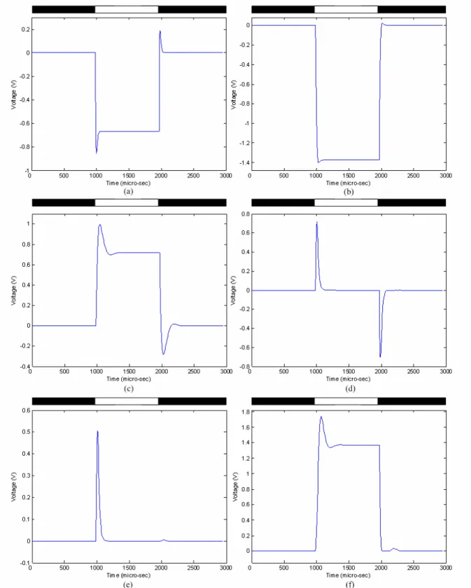
(34) into the one block OFFBIP in the macromodel, as can be seen in Fig. 2.3. The constants of OFFHELP and OFFBIP were also merged into a single time constant, τBPF. The two values in τBPF denote the upper and lower 3dB time constants. Fourth, the time constant of the blocks PH1 and H, were modified to τL, and that of block PH2 was modified to 4τL to facilitate chip implementation. For the same reason, the higher 3dB time constant of block OFFBIP was changed to 4τL, and the lower 3dB time constant of block OFFBIP was changed to τH, respectively. Finally, since the time constants of the amacrine cell and the ganglion cell were smaller than those of the ON and OFF bipolar cells, their neglect had no effect on the signal flow. Therefore, the time constants of the blocks Ama and GC were removed in the macromodel.. 2.3. SIMULATION RESULTS The RC equivalent circuit in Fig. 2. 1 is used to construct a 32x32 array which is simulated by. HSPICE. Since the array size is differs from the original definition of the space constants D, all the space constants in the simulation are shrunk with the same factor, 32/180. The simulation results are shown in Fig. 2. 4 ~ Fig. 2. 6. In this simulation, a voltage pulse is applied to the 5x5 cells in the center of the array to imitate the 500Hz flashing light stimulus and the spatiotemporal patterns of the 17th row are observed. First we show the transient response of the circuit when a pulse-stimulus is supplied. Fig. 2. 4 shows the output currents of the center cell of the 2-D array. The simulation is performed under the condition that a pulse signal with a turned-on duration of around 1ms is incident on the middle six cells of the array. The simulated input to the middle six cells are periodic stimulus with 100pA transient current added to a 100pA background-induced DC current. All other twenty-six cells are supplied with background currents of 100pA. All above-mentioned currents are supplied to the bases of the photo-BJT of all cells. The output of photoreceptor in Fig 2. 4(a) has overshooting and undershooting at the turn-on and turn-off similar to the CNN model simulation results in the 18.

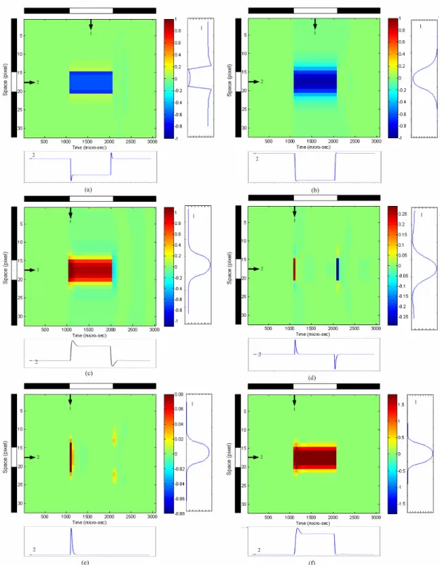
(35) previous section. It is also clear in Fig. 2. 4(b) that the output of the horizontal is analogous to that of the PH1 but has a larger magnitude. As mentioned in the previous section, the gate bias of MSM11, MSM12, MSM21, MSM22, MSM31, MSM32, MSM41, MSM42, MSM51, MSM52, MSM61 and MSM62, VSM, controls the diffusion range of the horizontal, on bipolar cell, off bipolar cell, amacrine cell and ganglion cell, respectively. Fig 2. 5 shows the steady state output of space domain response with subjected to suitable gate bias voltages of VSM. Fig 2. 5(b) is the results of the horizontal when the middle six cells are incident with stronger light while the other cells are incident with background light. As could be seen in the figure, a higher gate biasing voltage, VSM, causes lower resistance of the smoothing network, and a wider diffusion range is achieved. The results of photoreceptor with the same stimulus are shown in Fig 2. 5(a). As discussed previously, the edge of the incident pattern would have higher contrast in the output of PH1 but the extent of contrast varies with different diffusion range. In Fig. 2. 6, the x-axis is time and the y-axis is the pixel location which denotes space. The black and white bars denote the spatial and temporal region of the input stimulus. The stimulus is applied to the 15th to the 20th pixel from 1001 µsec to 2000 µsec. The waveform at the right of each pattern is the spatial domain waveform(s) obtained at the time marked by the vertical arrow(s). The waveform at the bottom of each pattern is the temporal domain waveform obtained at the location marked by the horizontal arrow. Fig. 2. 6(a) and (b) represent the spatiotemporal patterns of the photoreceptor and horizontal cell, respectively. It can be seen from Fig. 2. 6(a) that the photoreceptor‘s signal level drops when there is a stimulus, and it returns to its original level when the stimulus disappears. Slight undershooting and overshooting in temporal domain can be expected in the periphery as it reacts to the stimulus directly. In the spatial domain, there is strong contrast at the edge of the stimulus. At the edge pixels inside the stimulus, the signal level is higher than the other stimulated pixels. Contrarily, at the edge pixels where the stimulus is just absent, the signal level is higher than the other silent pixels. Therefore, the spatial range of the stimulus can be well 19.

(36) defined. In the temporal domain, the horizontal cell has a similar reaction to the photoreceptor, as can be seen in Fig. 2. 6(b). However, since the horizontal cell performs lateral diffusion in space, its spatial domain waveform spreads wider than that of the photoreceptor. Fig. 2. 6(c) and (d) represent the spatiotemporal patterns of the ON and OFF bipolar cells, respectively. The OFF bipolar cell performs bandpass-filtering on the signals from the photoreceptor. In the amacrine cell, the rectified signals from off bipolar cell with a gain factor, as shown in Fig. 2. 6(e). Moreover, the response to the appearance of the stimulus is weaker than the response to the disappearance of the stimulus. Thus the amacrine cell provides a strong inhibition to the ganglion cell when the stimulus disappears in time. Therefore, the ganglion cell exhibits clear turned-ON reaction, as can be seen in Fig. 2. 6 (f).. 20.

(37) Fig. 2. 1. The neuromorphic model of the ON sluggish sustain ganglion cell set of rabbits’ retinas. The parameter τ denotes the time constant in millisecond of the LPF. The parameter D denotes the space constant, which is defined by the laterally diffusing range in cell number in a 180-cell array.. Fig. 2. 2. The RC equivalent model of the ON sluggish sustain ganglion cell set of rabbits’ retinas. 21.

(38) Fig. 2. 3. The macromodel of a single pixel of the implemented chip.. 22.

(39) Fig. 2. 4. The HSPICE model-simulated time domain waveforms of the neuromorphic model of the ON sluggish sustain cell set in a 32x32 array for (a) photoreceptor, (b) horizontal cell, (c) ON bipolar cell, (d) OFF bipolar cell, (e) amacrine cell, and (f) ganglion cell. The light stimulus is applied at 1000th~2000th micro-second and Vsm = 2.2V.. 23.

(40) Fig. 2. 5. The HSPICE model-simulated space domain waveforms of the neuromorphic model of the ON sluggish sustain cell set in a 32x32 array for (a) photoreceptor, (b) horizontal cell, (c) ON bipolar cell, (d) OFF bipolar cell, (e) amacrine cell, and (f) ganglion cell. The light stimulus is applied at 15th~20th pixel and Vsm = 2.2V. 24.

(41) Fig. 2. 6. The HSPICE model-simulated time domain waveforms of the neuromorphic model of the ON sluggish sustain cell set in a 32x32 array for (a) photoreceptor, (b) horizontal cell, (c) ON bipolar cell, (d) OFF bipolar cell, (e) amacrine cell, and (f) ganglion cell. These waveforms are recorded from the 17th row of the array. The x-axis is normalized time and the y-axis is the pixel location which denotes space. The stimulus is applied to the 15th to the 20th pixel at time point 1001 to 2000. The waveform at the left of each pattern is the spatial domain waveform(s) obtained at the time marked by the vertical arrow(s). The waveform at the bottom of each pattern is the temporal domain waveform obtained at the location marked by the horizontal arrow. The Vsm = 2.2V. 25.

(42) CHAPTER 3 Circuit Design 3.1. ARCHITECTURE OF A BASIC CELL OF THE RETINAL CHIP Fig. 3.1 is the block diagram corresponding to the macromodel in Fig. 2. 2. A vertically. parasitic p+-n-well-p-substrate BJT QPHO with a floating base is used as a photo-BJT. The photo-BJT traduces light stimuli into electrical currents. Then the photocurrent is read out, inversed, amplified by eight times, and sent to the block PH1. Then the PH1 signal is sent to PH2 and H to perform temporal delay and spatial diffusion, respectively. Then the signals from PH2 and H are fed back into PH1. Since the input of this circuit is a photocurrent, all signals in PH1, PH2, and H are in current-mode. An additional cascode current mirror (denoted by sub-block CM) is used to inverse it and send it to the OFF bipolar cell (OFFBIP) in order to achieve the inverse band-pass-filtering function. The output current ION of PH1 directly enters the ON bipolar cell (ONBIP). Since the retina operation is very slow, very low frequency BPFs (denoted by sub-block BPF) are needed for the bipolar cells. For OFF bipolar cell, the current-mode signals from PH1 and CM are converted into voltage-mode signals by Rm amplifiers (denoted by the sub-block Rm Amp.) and fed into the BPF sub-blocks. The output signals of the sub-blocks BPF are converted to current-mode signals again using the sub-blocks V-I converter. The absolute-value circuits (denoted by the sub-block ABS) are used to rectify the bipolar cell signals. At the amacrine cell (Ama), the positively rectified signals of the OFF bipolar cells with a gain factor. The ganglion cell (GC) subtracts the amacrine cell’s signal from the positively rectified signal of the ON bipolar cell. Another sub-block ABS is used to rectify the ganglion cell’s signal in order to realize the complete function of the ON sluggish sustain ganglion cell set. There are six smoothing networks at the horizontal cell, ON bipolar cell, OFF bipolar cell, amacrine cell and ganglion cell, respectively, which are used to realize the space constants of these six cells. The space constants are realized by using tunable NMOSFET smoothing networks [4]. Such a technique can control the space constants by controlling the gate biases of the NMOSFETs, thus allowing greater flexibility in designing the space constants. Moreover, since the 26.

(43) horizontal cell has a relatively large space constant compared with the other cells, the NMOSFETs used in its smoothing network have a larger W/L ratio than the other five cells, as shown in Table II. The detailed transistor-level circuit of a pixel is shown in Fig. 3. 2 (a)-(d), and the transistor sizes are listed in Table II.. 3.2. CIRCUIT DESIGN OF THE BASIC CELL. 3.2.1 Photoreceptor and Horizontal cell Fig. 3. 2(a) represents the circuit of the photoreceptor (PH1 and PH2) and horizontal cell (H). Each block is constructed basically using cascode current mirrors to deal with the light-induced photocurrent. Because the photocurrent is around one hundred-pA to several hundred-nA, it can benefit from the good linearity of cascode current mirrors. Moreover, since the photocurrent might flow in or out of the circuit, complementary current mirrors are used to enable both current directions. The transistors M1-M6 are used to bias the emitter of QPHO at VB1 and to direct the photocurrent into the circuit. The transistors M7 - M18 provide a current gain of -8, as described in Fig. 3. 1. The CMOS transmission gates composed of transistors MPLP1-MPLP12 and MLPON1-MLPON8 in Fig. 3. 2 (a) and (b) are used as resistors. Their resistances are controlled by VNLP1 and VPLP1 for NMOSFET and PMOSFET, respectively. The resistances and the gate capacitances compose the LPF time constants of the blocks PH1, PH2, H, and ONBIP. The unit LPF time constant τL can be controlled by VNLP1, 2 and VPLP1, 2 simultaneously. On the other hand, the ratios of time constants can be set by designing the MOSFET’s sizes to get the suitable gate capacitances. The current mirror composed of transistors MPH11-MPH14 and MPH15-MPH18 is designed to have a current gain of four times. Thus the current of block PH1 is enlarged to enter block H. The enlarged current is spread by a diffusion network controlled by VSM, and then it is fed back to the block PH1 by another complementary current mirror, including transistors MH1-MH16. On the other hand, the current of the block PH1 is directly repeated to enter the block PH2 via the current mirror. Complementary current 27.

(44) mirror including transistors MPH21-MPH24 is used to perform the temporal delay and to send feedback to the block PH1. Therefore, the channel length and width of transistors MPH21, MPH22, MPH23, and MPH24, are both twice as large as those of MPH11, MPH12, MPH13, and MPH14. Thus, the current gain is kept as unity because the W/L ratio doesn’t change. However, the time constant of the block PH2 is four times larger than that of the block PH1 because the gate capacitances of MPH21 and MPH24 are four times larger than those of MPH11 and MPH14. The output current of block PH1 is enlarged four times by the current mirrors composed of transistors MPH11-MPH14, MCM1-MCM4, MCM5-MCM12 and MCM13-MCM16 to be sent to the bipolar cells. Transistors MCM1-MCM12 generate ION, which is to be sent to the block ONBIP. The drain current of transistors MCM2 and MCM3 is inversed using a complementary current mirror (CM). Transistors MCM1-MCM8 and MCM13-MCM16 generate IOFF, which is to be sent to the block OFFBIP. The drain current of transistors MCM2 and MCM3 is inversed using a complementary current mirror (CM). At the output stage, the transistors MO1 and MO2, MO3 and MO4, and MO5 and MO6 are used to repeat the output currents of the blocks PH1, PH2, and H, respectively, to enable chip measurement. Since there are external biases applied to measure the chip, simple structure instead of the cascode type slaves are used to save the pixel area.. 3.2.2 On bipolar cell The CMOS transmission gates composed of transistors MLPON1~ MLPON4 and MLPON5~ MLPON8 are used as transistors. Their resistances are controlled by VNLP2 and VPLP2 for NMOSFET and PMOSFET, respectively. The ratios of time constants can be set by designing the MOSFET’s sizes to get the suitable gate capacitances. Transistors MON1~MON8 are used to perform the temporal delay and to send feedforward to block Ama FB. The function of amacrine feed-back cell is to generate a low-passed signal from on bipolar cell’s output with a large time constant coefficient, τ , and then to feed the low-passed signal back to on bipolar cell for subtraction.A couple of current mirrors are used to realized amacrine feed-back 28.

(45) cell for subtraction. This generates undershoot and overshoot waveforms similar to biological measurements. To realize the architecture, we need a low-pass filter with a large time constant. A circuit named “continuous time current delay element” is used to implement the current-mode low-pass filter. The current delay element is a current mirror with a capacitor connected between the gates and sources of the two MOSFET. The result of current subtraction at the drain of MON26 andMON27 are then passed to a modified absolute value circuit (ABS) composed of the transistors MON29~ MON35. Transistors MON29~MON32 form a simple current mirror, and transistors MON33 and MON34 play the roles of adjustable switches that are controlled by VabsN and VabsP, respectively. The transistor MON33 sends the positively rectified signal of the block ONBIP to the block GC as ION_GC.. 3.2.3 Off bipolar cell The circuit of the off bipolar cell stage is shown in Fig. 3. 2(c). At the OFFBIP path, an Rm amplifier composed of transistors MRM1-MRM4 is used to transduce the current IOFF into voltage-mode. Afterward, a poly capacitor COFF and a CMOS transmission gate, including transistors MHP1 and MHP2, are used to form a highpass filter (HPF). This HPF and the LPF composed of MPLP13, MPLP14, and MVI1 form the sub-block BPF. The bandwidth of the HPF, which is also the lower 3dB time constant of the BPF τ, can be tuned by the biases VNHP and VPHP at gates of MHP1 and MHP2, respectively. The transmission gate is connected to the reference bias Vref, which is set to a half of the supply voltage to balance both upward and downward signal swings. The voltage-mode signal of the sub-block BPF is transduced into the current-mode signal again by using a transconductor composed of transistors MVI1-MVI10 [25]. The transconductor is a low-voltage low-power class-AB linear transconductor [26]. Its positive input node connects to the output of the sub-block BPF, and its negative input node connects to the reference bias Vref. The circuit performs as a linear transconductor but it works in class-AB. This is due to the FVF (flipped voltage follower) [27] low impedance buffers that only force the current of the circuit under quiescent conditions, and 29.