國
立
交
通
大
學
多媒體工程研究所
碩
士
論
文
以 骨 架 驅 動 之 交 互 參 數 化
Skeleton-Driven Cross-Parameterization
研 究 生:廖仁傑
指導教授:莊榮宏 教授
黃世強 教授
中 華 民 國 一百 年 十 月
以骨架驅動之交互參數化
Skeleton-Driven Cross-Parameterization
研 究 生:廖仁傑 Student:Jen-Chieh Liao
指導教授:莊榮宏 Advisor:Jung-Hong Chuang
黃世強 Wingo Sai-Keung Wong
國 立 交 通 大 學
多 媒 體 工 程 研 究 所
碩 士 論 文
A Thesis
Submitted to Institute of MultimediaEngineering College of Computer Science
National Chiao Tung University in partial Fulfillment of the Requirements
for the Degree of Master
in
Computer Science
October 2011
Hsinchu, Taiwan, Republic of China
以骨架驅動之交互參數化
研究生 : 廖仁傑 指導教授 : 莊榮宏 博士
黃世強 博士
國立交通大學
資訊學院多媒體工程研究所
摘 要
我們提出一個以骨架資訊來產生兩三維物體間交互參數化之方法。給予兩個物 體,我們擷取出其骨架並取得骨架與物體表面間、以及骨架與骨架間之對應資 訊。兩物體接著會透過切割程序分成數個相對應的區塊,接著我們將每一個對應 的區塊分別參數化到一個平面上。而每一參數化之分割區塊,我們則透過一個迭 代放鬆法來產生分割區塊間之交互參數化,此迭代放鬆法主要由骨架與表面以及 骨架與骨架間之對應資訊來驅動。兩物體分割區塊之交互參數化產生後,我們於 分割區塊之邊緣處使用一個平滑化的程序來產生出最後的對應結果。概要來說, 我們使用了密集的骨架與物體表面間之對應資訊當作軟性限制來建立交互參數 化。相較於先前之技術,此方法可以自動的產生出物體間有意義之特徵對應且無 須給予對應限制點,並僅需提供少量之對應點在分割區塊的邊緣處即可。此方法 也可以自動的產生出特徵的部分對應。 iSkeleton-Driven Cross-Parameterization
Student: Jen-Chieh Liao
Advisor: Dr. Jung-Hong Chuang
Dr. Wingo Sai-Keung Wong
Institute of Multimedia Engineering
College of Computer Science
National Chiao Tung University
ABSTRACT
We propose a novel skeleton-driven framework for cross-parameterization between two 3D polygonal models. Given two models, we first extract their curve skeletons, retrieve the skeleton-to-surface mapping information, and derive a skeleton-to-skeleton mapping. We then segment both meshes into several consistent parts and for each part pair we embed the parts in cor-respondence onto a planer domain. After the process of embedding, we apply an iterative relaxation scheme on each parameterized part that takes the to-surface and skeleton-to-skeleton mapping information into account. A smoothing process is invoked at the end so as to smooth the cross-parameterization along the part boundaries. Briefly speaking, we use the dense skeleton-to-surface mapping information as the soft constraints during the cross-parameterization construction. As a result, our method can match the object features automati-cally without the general feature constraint points as common approaches. The method requires only a few user inputs that specify matching points on the part boundaries. We also show that our method can generate partial mapping results for the models that have unique object features.
Acknowledgments
I would like to thank my advisors, Professor Jung-Hong Chuang and Wingo Sai-Keung Wong, for their guidance, inspirations, and encouragement. I am also grateful to my senior colleague, Tan-Chi Ho for his enlightenment and generously sharing his research works, such as PMLab and MSP skeleton. I-Cheng Yeh help us generate all kinds of testing results we ask with the approach he proposed. And then I want to appreciate my brother Jen-Chieh Liao for his kind assistances, useful suggestions and help me figure out the rendering related questions. I would like to thank to all my colleagues in CGGM lab: Cheng-Guo Huang, Shao-Ti Lee, Bo-Yin Yao, Mu-Shiue Li, Yi-Shan Li for their patient listening and discussing with me on the research issues. Tsung-Shian Huang helps me understand much rendering knowledge, and all my junior colleagues’ kind assistances. Thanks to International Games System CO., LTD. for offering me research scholarship. I especially want to thank my parents for their love, support, care and tolerance. Without my parents, I could not pass all the frustrations and pain in my life.
Contents
1 Introduction 1
1.1 Contributions . . . 3
1.2 Organization of the thesis . . . 3
2 Related Work 4 2.1 Shape correspondence . . . 4
2.2 Skeleton correspondence . . . 5
2.3 Cross-parameterization . . . 6
2.3.1 Base complex method . . . 6
2.3.2 Deformation-driven method . . . 8
2.3.3 Hybrid method . . . 8
3 Algorithm 11 3.1 Overview . . . 12
3.2 Skeleton extraction and mapping construction . . . 13
3.3 Consistent segmentation . . . 14
3.3.1 Skeleton-driven segmentation . . . 14
3.3.2 Part boundary growing and refinement . . . 15
3.4 Cross-parameterization . . . 16
3.4.1 Initial embedding . . . 17
3.4.2 Relaxation . . . 20
3.5 Part boundary smoothing . . . 22
3.5.1 Hint position generation . . . 23
3.5.2 Shape preserving generation of base mesh . . . 24
3.5.3 Deformation and re-projection . . . 27
4 Experimental Result 31 4.1 Result . . . 31 4.2 Timing information . . . 55 5 Conclusions 56 5.1 Summary . . . 56 5.2 Limitations . . . 57 5.3 Future works . . . 60 Bibliography 61 iv
List of Figures
2.1 An example of shape correspondence . . . 5
2.2 An example of least-squares mesh [MAN08] . . . 9
3.1 System overview . . . 12
3.2 Circular parameterization domain and its mapping to each other . . . 15
3.3 Part boundary refinement . . . 16
3.4 Overview of the cross-parameterization computation for two parts . . . 17
3.5 The differential coordinates . . . 18
3.6 The illustration for the orientation adjustment . . . 19
3.7 Mapping error . . . 21
3.8 Interquartile Range (IQR) . . . 22
3.9 Hint position generation . . . 23
3.10 The cross-parameterization step in [WPZM10], which maps a lion model to its own convex hull. (a) lion model (b) convex hull cross-parameterization com-puted using the uniform representation (c) convex hull cross-parameterization computed using the mean-value Laplacian representation . . . 25
3.11 The illustration of the vertex without mapping position . . . 25
3.12 Base mesh generation . . . 26 3.13 Mapping from a dog (a) to a wolf (b), (c) after deformation (d) after re-projection 29
3.14 Mapping vertices and edges of the dog model before part boundary smoothing
(different edge color represents different parts) . . . 29
3.15 Mapping vertices and edges of the dog model after part boundary smoothing (different edge color represents different parts or the overlapping regions) . . . 30
4.1 The visualization of skeleton-to-surface mapping of the dog model . . . 32
4.2 The visualization of skeleton-to-surface mapping of the wolf model . . . 32
4.3 The visualization of the skeleton-to-surface mapping slices . . . 33
4.4 The skeleton node correspondence between the dog and wolf model . . . 34
4.5 The skeleton-to-skeleton mapping between the dog and wolf model . . . 34
4.6 The segmented parts and matching points colored in red and blue specified on the part boundaries . . . 35
4.7 The cross-parameterization between the dog and wolf model . . . 35
4.8 The cross-parameterization of the heads between the dog and wolf model . . . 36
4.9 The cross-parameterize result of the limbs between the dog and wolf model. (a) front legs (b) back legs . . . 36
4.10 The twist effect due to the lack of the orientation information on the slice region 37 4.11 The cross-parameterization between the lion and cat model . . . 37
4.12 The cross-parameterization of the head part between the lion and cat model . . 38
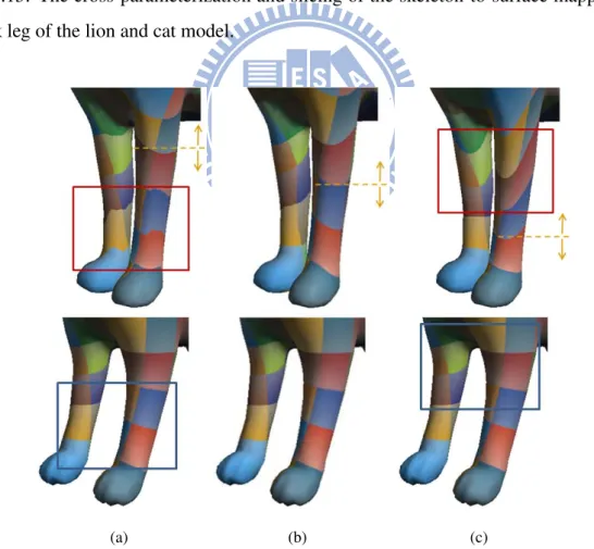
4.13 The cross-parameterization of the front legs between the lion (top) and cat (bot-tom). The texture repeat cycle is doubled from left to right to clarify the result . 38 4.14 The cross-parameterization of the back legs between the lion (top) and cat (bot-tom). The texture repeat cycle is doubled from left to right to clarify the result . 39 4.15 The cross-parameterization and slicing of the skeleton-to-surface mapping of the left back leg of the lion and cat model . . . 40
4.16 The cross-parameterization of the front legs between the lion (top) and cat (bot-tom) model with different cut positions. (a) upper one-third (b) middle (c) lower one-third . . . 40
4.17 The cross-parameterization between the horse models in the standing pose and in normal pose . . . 41 4.18 The cross-parameterization between the head parts of the horse model in
differ-ent poses . . . 42 4.19 The cross-parameterization between the left front legs of the horse models in
different poses . . . 42 4.20 The mapping result from a long ear cat head to the lion head with different
mapping error weights . . . 43 4.21 The mapping result from a long ear cat head to the lion head with different
stretch error weights . . . 44 4.22 The cross-parameterization between the long ear cat head and lion head (side
view) . . . 45 4.23 The cross-parameterization between the long ear cat head and lion head (front
view) . . . 45 4.24 The cross-parameterization between the long ear cat head and lion head (top view) 46 4.25 The cross-parameterization between the dragon and wolf model . . . 47 4.26 The cross-parameterization of the head part between the dragon and the wolf
model . . . 47 4.27 The cross-parameterization of the limbs between the dragon and wolf model.
(a) right front leg (b) left front leg . . . 48 4.28 The cross-parameterization of the limbs between dragon and wolf model. (a)
right back leg (b) left back leg . . . 48 4.29 The cross-parameterization of the tail part between the dragon and wolf model . 49 4.30 The visualization of slice mapping from the dragon to the wolf model . . . 49 4.31 Skeleton node correspondence between the dragon and wolf model . . . 50 4.32 Partial mapping of horns from the dragon to the wolf model . . . 50 4.33 Partial mapping of the left two claws from the dragon to the wolf model . . . . 51 4.34 Partial mapping of the right two claws from the dragon to the wolf model . . . 51
4.35 Partial mapping of tails from the dragon to the wolf model . . . 51 4.36 The slicing of the skeleton-to-surface mapping of the camel and the horse model 52 4.37 The cross-parameterization between the hose and camel model . . . 53 4.38 The cross-parameterization of the body between the horse and camel model . . 53 4.39 The cross-parameterization of the limbs between the horse and the camel model.
(a) front legs (b) back legs. The dotted lines represent the approximate segmen-tation positions in the segmensegmen-tation process . . . 54 4.40 Partial mapping of tail from the camel to horse model . . . 54 5.1 L2 stretch can not recognize the distortion caused by the rotation along the
indicate direction . . . 58 5.2 Illustration of orientation angle calculation . . . 59 5.3 The folding phenomenon in the parameterization domain . . . 60
C H A P T E R
1
Introduction
A cross-parameterization (or inter-surface mapping) between different shapes is a fundamental task in a number of applications, such as object recognition, shape morphing or blending, texture and surface feature transfer, pair-wise model editing, and geometry remeshing. The cross-parameterization establishes a bijective mapping between the vertices of the given meshes by mapping vertices onto an identical domain or by mapping one mesh onto another directly.
Several cross-parameterization methods have been proposed in the last decade. These meth-ods require a set of correspondent points to be specified as constraints for generating the cross-parameterization between the given models. The corresponding constraint points are obtained either by using automatic methods or by the users. The automatic method finds the constraint points by taking the local saliency value and the closeness of the point to the tip areas into account. Since the finding criterion of the automatic method is quite simple, directly using the constraint points generated by the method usually can not generated satisfying mapping results. Therefore, common approaches require the users to specify corresponding constraint points manually. Users need to indicate the constraint points on the areas that are geometrically or perceptually important such as eyes, mouths, or the tip of the limbs. Also, the mapping result
2
can be enhanced by specifying more corresponding constraint points manually. But when the number of the corresponding constraint point increases, the complexity of the geometrical and topological operations raises [KS04, SAPH04]. Also, in order to obtain a satisfactory cross-parameterization result, user often needs to specify numerous corresponding constraint points between the two models. This could be time consuming and tedious. When the models have unique features (e.g. one has a tail and the other has not), user often needs to specify additional constraint points to achieve reasonable partial mapping results. Yet, to specify such constraint points around the area that has no apparent features may not always be intuitive.
According to the survey paper [vKZHCO10], to semantically correspond two different mod-els, we usually need a high-level descriptor to improve the correspondence. For example, Shalom et al. [SSSCO08] use the shape-diameter function (SDF) to partition the models and use it to find the corresponding parts in other objects. Hu et al. [HLW09] assign each seg-ment part a bone and correspond the segseg-ment parts of the models by adopting a graph matching technique on the skeleton graphs. Our motivation is to find a high level descriptor to assist the computation of the cross-parameterization between the given models. Skeleton is an ap-propriate choice since it represents the global structure of a model and is not sensitive to the local surface noise. Several skeleton corresponding schemes also have been proposed in the last decade. The other information we need is the meaningful dense mapping information be-tween the skeleton and the surface. Although there exist many skeletonization methods that can produce skeleton-to-surface mapping information, these methods lack of the consideration for the surface features. However, some skeletonization methods proposed recently can encode the surface shape features onto the skeleton nodes and fill the lack. Ho [Ho11] extracts the skeleton by iterative shrinking the mesh using the minimum slice perimeter function, which encodes the local shape information associated with the surface points. This provides dense mapping infor-mation between the skeleton and the surface that approximately matches the human perception. Therefore, we may have a chance to construct the cross-parameterization between the models by utilizing the skeleton-to-skeleton and skeleton-to-surface mapping information. With this in-formation, we can compute the mapping difference for each vertex by measuring the mapping
1.1 Contributions 3
difference on the skeletons. Since skeleton is a set of line segments, measuring the mapping difference on the skeletons is much easier than directly compute it on the surfaces. Also, it does not affect by models which have extremely different orientations or poses. With the dense mapping information encode on the skeletons, we can match the object features well without users to specify corresponding constraint points.
1.1
Contributions
The main contributions of our work are:
• The method can achieve cross-parameterization results that match the object features. • The method performs well on the models with significant different part sizes or shapes. • The method requires only a few orientation adjustment points specified by the users
man-ually.
1.2
Organization of the thesis
The following chapters are organized as follows. Chapter 2 gives the review and the back-ground knowledge of the previous researches. Chapter 3 describes our cross-parameterization algorithm, including the overview, skeleton extraction and mapping, part segmentation, cross-parameterization and part boundary smoothing. Chapter 4 shows the experimental results of our cross-parameterization algorithm with several different visualizations. We summarize our cross–parameterization algorithm and discuss its limitations and future works in Chapter 5.
C H A P T E R
2
Related Work
In this chapter, we review the previous work of shape correspondence and cross-parameterization.
2.1
Shape correspondence
Shape correspondence establishes a meaningful correspondence between geometric elements of the given objects. The types of element may be mesh primitives, surface feature points, skeletal features, or local parts of the model. The correspondence between the geometric elements can be one-to-one, one-to-many, or many-to-many. Figure 2.1 shows an example of a one-to-one correspondence of the surface feature points between two objects. Since the objects may have large difference in pose, shape, and surface detail, establishing the correspondence based on the similarity of local geometric information can be difficult. Higher level descriptors which can describe the global structures of the objects and semantics of the parts help to overcome this problem.
According to the survey presented by Kaick et al. [vKZHCO10], the shape correspondence problem can be categorized into similarity-based correspondence, rigid alignment, non-rigid
2.2 Skeleton correspondence 5
Figure 2.1: An example of shape correspondence [ZSCO+08].
alignment, and time-varying registration. The skeleton correspondence and cross-parameterization problem are a part of the similarity-based correspondence.
2.2
Skeleton correspondence
Curve skeleton is a common shape descriptor since it represents the global structure of a 3D shape and is insensitive to the surface noises. Therefore, to generate the skeleton correspon-dence between the given models can be efficient. Several methods utilize the skeleton or reeb graph to solve the matching problem. Sundar et al. [SSGD03] performed a greedy and depth-first search scheme to find the bipartite graph that has maximum cardinality and minimum weight between the two skeleton graphs. Biasotti et al. [BMSF06] constructed the partial shape-matching by finding the maximum common sub-graph between the two reeb graphs. The sub-graph is able to recognize the similar sub-parts of the objects represented as 3D polygonal meshes. Both methods match the common subgraphs by searching along graph connectivity. Therefore, they are either sensitive to topological differences or require complicated strategies to edit the topological structures. Au et al. [ATCO+10] used a voting scheme to handle the topological difference and the symmetry switching problems. They employ the combinatorial search and local topology consistency pruning test to filter out the poor correspondences which
2.3 Cross-parameterization 6
have large topological differences. The multidimensional scaling (MDS) [EK03] is invoked to straighten the skeletons so as to deal with the pose variant condition. Since the algorithm is purely geometric-based, unaware of the semantics of parts. It may mismatch components with different semantics but similar geometry. Liu [Liu10] extended the work of [ATCO+10]
by adding symmetric detection, structure diagnosing, and spatial configuration into the system. These information help to overcome the large structural difference or topology noise causing by gluing, enhance the correctness of partial correspondence, and handle the condition of the com-posite object. Since the objective function considers not only curve skeleton but also surface information, it can also recognize the relative position of the corresponding groups.
2.3
Cross-parameterization
Cross-parameterization methods can be divided into three major categories: base complex method, deformation-driven method, and hybrid method.
2.3.1
Base complex method
Usually, it is hard to directly construct the inter-surface mapping between the two models since the models are often different in orientation, object feature, and surface local feature. Therefore, most of the cross-parameterization methods generate the inter-surface mapping through an in-termediate common parameterized domain. The construction can be summarized as three major steps: First, an intermediate common domain is found. Second, each model is embedded into the common domain separately and the correspondence between the common domain and the model is derived. Third, the inter-surface mapping between the models is constructed through the composition of the common domains.
Several methods use the base complex as the intermediate domain. Lee et al. [LDSS99] generated the coarse mesh as a simplicial complex that retains the user select feature points by using MAPS [LSS+98]. Since the coarse meshes of the source and target does not guarantee to have the same topology connectivity. An alignment and projection is adopted to construct the
2.3 Cross-parameterization 7
correspondence map between the coarse meshes. And an iterative relaxation procedure and user adjustment is invoked to produce the final inter-surface mapping. Usually, this method does not suit the models that differ greatly in shapes. Therefore, later methods use the consistent segmen-tation to found the coarse meshes. The consistent segmensegmen-tation guarantees the coarse meshes of the source and target models having the same topology. As a result, each segment patch can be directly corresponded to the other without alignment and projection. In the proposed method of Praun et al. [PSS01], user specified corresponding constraint points and their connectivity as in-put, the method partitioned a mesh into triangular patches by tracing the paths along the surface. The correspondence of each vertex is then constructed according to its lying patch. Kraevoy et al. [KS04], and Schreiner et al. [SAPH04] extend the methods of [PSS01] to construct the simplicial complex and retrieved the patches automatically. Both methods required correspond-ing constraint points specified by user only. Kraevoy et al. [KS04] mapped the surfaces onto the patches through the shape preserving parameterization method proposed by Floater [Flo03] to generate the mapping from the surface to simplicial complex. Schreiner et al. [SAPH04] used an alternative approach that does not compute an explicit map between the surface and simplicial complex. Instead, they directly create and optimize a continuous map between the meshes. The inter-surface mapping is constructed by minimizing the map distortion during the interleaved coarse-to-fine refinement of both meshes. Pan et al. [PWPY07] adopted the method of [KS04] and enhanced the cross-parameterization results by adjusting the simplicial complex iteratively according to the previous generated result.
For the base complex method that construct triangular patches on the meshes [PSS01, KS04, SAPH04, PWPY07], often cannot avoid complicated geometric and topological operations. Which intend to prevent intersections and blocking, to reach consistent cyclic orders and to avoid swirls. Furthermore, they usually need to deal with the discontinuity between the patch boundaries with additional smoothing process. These operations are time consuming and un-stable for complex shapes.
2.3 Cross-parameterization 8
2.3.2
Deformation-driven method
Several methods use the deformation-driven approach for deriving cross-parameterization. Deformation-driven approach directly deforms one mesh to the other by minimizing some energy functions.
The energy function consists of components that pull the vertices of one mesh towards the de-sired location while preserving the shape of the mesh. Usually, the deformation process requires user to specify several corresponding constraint points between the input models.
Allen et al. [ACP03] used a template fitting technique to construct the cross-parameterization for a set of human models in the same pose by minimize a error metric that measures the dis-tance from each vertex to the target surface, the difference in the affine transformation matrix, and the closeness of the corresponding constraint points. But optimization can easily converge to a poor local minimum for the models that differ greatly in shapes. Sumner and Popovic [SP04] used a method similar to [ACP03] and changed the feature matching term into an iden-tity transformation constraint, which intends to prevent the method from generating a drastic change in the shape of the mesh and to achieve optimal smoothness. However, both methods require the source and the target models to be similar in the shape and the pose. Hu et al. [HLW09] solve this problem by segmenting the models into consistent parts and computing the cross-parameterization for each part independently using the method of [ACP03]. Each parts are then combined together to generate the final results. Wu et al. [WPZM10] generated the model transduction between two models by deforming the source model to the target model. They replaced the general Laplacian differential coordinate term that used in the deformation process with the mean value coordinate proposed by Floater [Flo03]. Since the mean value coordinate encodes the shape features. This approach preserves the local shape detail of the source model during the deformation process and enhances the cross-parameterization results.
2.3.3
Hybrid method
When the models differ greatly in shape or pose, deforming one model to the other directly may generate unsatisfied result since the optimization converges to a poor local minimum. Recent
2.3 Cross-parameterization 9
work [MAN08, WPZ+11, YLSL11] constructs the cross-parameterization by using the hybrid approach, which can be summarized in two major steps: First, the source and the target mod-els are mapped onto a coarse mesh, respectively. Second, the cross-parameterization is then generated via the mapping obtained by deforming one coarse mesh to another coarse mesh.
Matsui et al. [MAN08] first deformed the models into a shrink-like coarse mesh using the least-squares mesh (LS-mesh) [SCO04] as shown in Figure 2.2, and generated the final cross-parameterization by applying an iterative closest point learning algorithm on the LS-meshes. Wu et al. [WPZ+11] segmented the input meshes into consistent parts and mapped each of
them onto a convex hull. The convex hull is then deformed into the other one by minimizing the energy function similar to [WPZM10]. The inter-surface mapping between the parts is gener-ated through the composition of the mappings from a convex hull to a part. Yeh et al. [YLSL11] also generated LS-meshes of input models as coarse meshes. The method first deformed one coarse mesh to the other coarse mesh obtain the initial coarse fitting. Second, they performed an fine fitting to generate the cross-parameterization. The fine fitting found the additional reli-able correspondences automatically and deformed the source mesh further to match the shape features greatly. They also proposed a dual-domain mesh relaxation method to greatly avoid or eliminate the problem of pinching and foldover artifacts during the deformation process.
2.3 Cross-parameterization 10
Although the recent work of cross-parameterization can generate satisfactory global struc-ture mapping between the models, there is still room for improvement. In the case of the given models have extremely different size of the object parts, these methods usually require more corresponding constraint points to be specified in order to generate the desired mapping. In addition, the minimum required number of the corresponding constraint points and their placement to generate the satisfactory results is quite ambiguous. Therefore, we propose a fast method which can construct the cross-parameterization between the models that is able to well match both the global features and the object features of the models based on only a few match-ing points specified by the users. It requires only one to two matchmatch-ing points on the segment part boundaries, which are quite intuitive and easy to specify.
C H A P T E R
3
Algorithm
In most of the cross-parameterization approaches, user needs to specify corresponding con-straint points on the given models to constrain the mapping in these regions. However, the minimum number of the feature points required and how to position there constraint points for generating the satisfactory results are quite ambiguous. This motivated us to develop a cross-parameterization method that does not need users to specify corresponding constraint points manually. We propose a skeleton-driven cross-parameterization algorithm that can gen-erate surface-to-surface mapping between given models with limited user intervention. Our method aims at constructing the cross-parameterization by using the information provided by the skeleton mapping and the surface mapping. The dense skeleton-to-surface mapping provides natural constraint information for feature correspondence.
To construct the cross-parameterization using such mapping information, we may encounter two major problems: First, we need to find a way to utilize the dense skeleton-to-surface map-ping information as constraints during the cross-parameterization computation. Since the con-straints are many, directly solve it using the deformation-driven methods may have no solutions or result in pinching and foldover artifacts. Second, the skeleton-to-surface mapping only
3.1 Overview 12
codes the shape features of the surface and lacks the orientation information. Therefore, we need to apply some additional constraints to handle this problem. To deal with the two prob-lems, we plan to embed the polygon meshes onto the planer domain. Under the planer domain, we can adopt an iterative local relaxation method to construction the cross-parameterization. The relaxation approach utilizes the dense mapping information as a guide to move each vertex to the reasonable parameterize position. And the insufficient orientation information problem can also be dealt by measuring the distortions of the embedded polygons.
3.1
Overview
skeleton extraction and mapping construction
consistent segmentation cross parameterization
part boundary smoothing
3.2 Skeleton extraction and mapping construction 13
Figure 3.1 shows the main steps of our cross-parameterization method, for given source and tar-get models, the first step extracts curve skeletons using the method proposed by [Ho11]. Note that the derived skeleton possesses a dense skeleton-to-surface mapping. Second, we construct the skeleton-to-skeleton mapping such that each skeleton node of the source (target) skeleton maps to a position on the target (source) skeleton. These two mapping information will be used later in the consistent segmentation and the parameterization process. Third, we segment both meshes into several consistent parts and to parameterize both parts onto the same intermediate planer domain. On the intermediate domain, we generate the surface-to-surface mapping be-tween parts by minimizing the stretch and mapping error through a relaxation process. Finally, we smooth the mapping along the part boundaries to compute the final cross-parameterization.
3.2
Skeleton extraction and mapping construction
The skeleton is extracted directly from a 3D model based on the so-called MSP function de-scribed in [Ho11]. MSP is a surface function that describes the internal local volume of the object around a surface point, and is used here to transform the original mesh to a shrunk skeleton-like mesh during the skeletonization process. With the approach of an iterative edge swap framework, this shrunk mesh then degenerates into a 1D curved skeleton. Instead of us-ing the traditional edge-collapsed operator, the edge swap operator is used to change the edge connectivity without simplifying the geometry. A compact error metric is used to measure the deviation of the shrunk mesh vertex. Under this guidance, a curved skeleton can be yielded with dense skeleton nodes which corresponding to a set of shrunk vertices. As a result, the skeleton generated by this MSP-driven method provides a dense skeleton-to-surface mapping in which each skeleton node corresponds to a set of shrunk vertices. This mapping information encodes the volumetric information on the skeleton and provides a natural constrain information for feature correspondence.
After the skeletons of the source and the target meshes are extracted, we establish the cor-respondence of the terminal and junction nodes between two skeletons either by the work of
3.3 Consistent segmentation 14
[Liu10] or manually. The skeleton nodes are mapping through a linear interpolation along the skeleton path. For those unique features that do not have the corresponding positions, we assign their correspondences to be same as the nearest corresponded node. For example, in Figure 4.31, the three protrusions on the dragon’s tail will be corresponded to the no.12 skeleton node of the wolf model.
3.3
Consistent segmentation
Since our system construct the cross-parameterization through a relaxation process, which itera-tively adjust the weight of the one ring vertices for each vertex. The new position for the vertices is compute through the weighting sum of the one ring vertices. In addition, we want to mea-sure the stretch during the relaxation process in order to overcome the orientation information deficiency problem. Therefore, we required the medium to be a 2D planer domain. To embed a polygon mesh into a planer domain without folding (as shown in Figure 5.3), the polygon mesh must have exactly one open boundary. Hence, we perform a consistent segmentation by using the skeleton-to-skeleton and the skeleton-to-surface mapping. The segmentation approach can be divided into two major steps, including skeleton-driven segmentation (Subsection 3.3.1) and part boundary growing and refinement for avoiding sinking vertices into local minimum in the relaxation process (Subsection 3.3.2).
3.3.1
Skeleton-driven segmentation
After the skeleton-to-skeleton mapping is established, we have a fully correspondence of the skeleton nodes between the source and target skeletons. Since each skeleton path represents a specific surface region of the mesh, it is easy to map the surface region between the source and target through the skeleton mapping. With this correspondence information, we can eas-ily segment the mesh into several parts by performing the segmentation on the skeleton. We analyze all the source skeleton paths and filter out the small skeleton paths which are related to the local structure such as mouth or ears. For the rest of the skeleton paths that relate to
3.3 Consistent segmentation 15
the main structure of the model (like neck, belly, limbs, etc), we cut each of them from the center to separate the skeleton paths into several segments. Since the center of a skeleton path usually refers to a surface region in cylinder shape, cutting at this position usually results in a low boundary distortion during the initial embedding (Subsection 3.4.1). After we finish the skeleton segmentation, we obtain the segment parts of the mesh simultaneously with each part corresponding to a specific skeleton limb. The segmentation on the target mesh can be obtained by simply transferring each cut node of the source skeleton to the target skeleton through the skeleton-to-skeleton mapping.
3.3.2
Part boundary growing and refinement
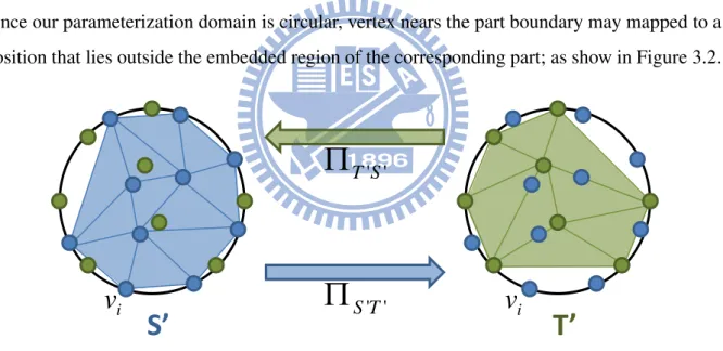
Since our parameterization domain is circular, vertex nears the part boundary may mapped to a position that lies outside the embedded region of the corresponding part; as show in Figure 3.2.
' 'T S
Π
' 'S TΠ
S’
T’
iv
v
iFigure 3.2: Circular parameterization domain and its mapping to each other.
To overcome the problem mentioned above as well as to smooth the mapping result along the part boundaries, we out grow the part boundaries such that adjacent parts overlap by a small region. Next, we refine the part boundaries to avoid the case that a triangle degenerats to a line during the parameterization process. We remove a triangle from the part if its two edges are on the part boundary path. If the removing the triangle will cause it to be isolated, we add the
3.4 Cross-parameterization 16
fan-shaped triangles between one of the triangle edges and the adjacent boundary edge into the part as shown in Figure 3.3.
Figure 3.3: Part boundary refinement.
3.4
Cross-parameterization
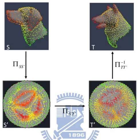
The correspondences between the source and target parts can be obtained after the part seg-mentation. Each part pair’s internal mapping is then constructed through the parameteriza-tion. As in Figure ??, the mapping is a composition of three consequent mappings: ΠST =
ΠSS0 ◦ ΠS0T0 ◦ Π−1
T T0, where ΠSS0 (ΠT T0) is the mapping from the source (target) mesh to its 2D circular parameterization domain. ΠS0T0 is the mapping from the source parameterization do-main S0to the target parameterization domain T0that simply maps each point in S0 to T0 using the parameterization position u(x, y) in S0. Therefore, our main purpose is to find a suitable parameterize position for each vertex of the parts to obtain the reasonable mapping on surface. To reach this goal, we proposed an iterative relaxation method, which is a two step approach consists of an initial embedding (Subsection 3.4.1) and a relaxation process (Subsection 3.4.2) as describe below.
3.4 Cross-parameterization 17 ' SS
Π
' 'T SΠ
1 ' −Π
TTS
T
S’
T’
Figure 3.4: Overview of the cross-parameterization computation for two parts.
3.4.1
Initial embedding
We embed the parts in correspondence into a 2D circular domain by using the mean value coordinates proposed by [Flo03], which is shape preserving and has low angular distortion. The boundary vertices of S are mapped into the boundary vertices of S0. For each inner vertex vi of S, its projected point ui on S0 is derived by minimizing the following local quadratic
energy: E(ui) = X (i,j)∈E wij(uj − ui)2, (3.1) where wij = tan(αij/2) + tan(βij/2) kvj − vik (3.2)
3.4 Cross-parameterization 18
is the mean-value coefficient, αij and βij are the angles shown in Figure 3.5. The optimal
i
v
ijβ
ijα
jv
Figure 3.5: The differential coordinates.
positions for uican be found by solving a sparse system of linear equations:
X
(i,j)∈E
wij(uj− ui) = 0 (3.3)
In order to have a better cross-parameterization, the embedding of source and target parts need to be adjust. This can be done by requiring users to specify a matching point on the bound-aries of the parts. As shown in Figure 3.6, users specify the matching point on the boundbound-aries of the source and target parts (ex: the bottom of the neck). Note that specifying these matching points are much easier and more intuitive than assigning the general corresponding constraint points to user. In our experience, one to two matching points are suitable in most cases.
For each vertex uiin the parameter domain let us define its stretch σi = σ(ui) by
σi = q X A(Tj)σ(Uj)2/ X A(Tj) (3.4) σ(U ) =p(Γ2+ γ2)/2 (3.5)
where A(T ) denotes the area of triangle T and the sums are taken over all triangles Tj
sur-rounding mesh vertex vi corresponding to ui, σ(U ) is the L2stretch for a embedded triangle, Γ
and γ are the maximal and minimal Eigen values of the metric tensor induced by the mapping [SSGH01]. To alleviate the L2 stretch of the embedded triangles and to have a more uniform
3.4 Cross-parameterization 19
matching point
S’ T’ T’
S T
without adjustment with adjustment
Figure 3.6: The illustration for the orientation adjustment.
distribution of the vertices on the parameterization domain. We relax the stretch of the embed-ding geometry with the previous work of [YBS04], which iteratively changing the edge weights for each vertex:
wnewij = w 0 ij P (i,j)∈Ew 0 ij , (3.6) where w0ij = w old ij σj , (i, j) ∈ E, (3.7)
and solving (3.3) to derive the new optimal positions. The process iteratively pushes each embedded vertex towards a direction with lower stretch. Therefore, embedded triangle with high L2stretch can be lowered by the replacement of the neighbor vertices.
Notice that we do not need to relax the stretch of the embedding geometry to the optimal result like [YBS04]. The main purpose of this approach is to prevent the embedding vertices from sinking into the local minimum of the following relaxation process. Since the control variable of the following relaxation process are the stretch error and the mapping error, which are defined in the following paragraphs, an extremely high stretch may dominant the relaxation
3.4 Cross-parameterization 20
process and let the mapping error to be merely effective.
3.4.2
Relaxation
After the initial part parameterization, the source and target part are embedded into a 2D circu-lar domain without folding. We proposed a relaxation approach to iteratively improve the result on the source and target. The main purpose is to push each embedded vertex towards a direction which leads to the position that has the reasonable mapping on surface. Using the same idea as [YBS04], each improvement step we adjust the one ring edge weight for each vertex of the pa-rameterization generated at the previous step. And the new optimal position for each embedded vertex is found by solving (3.3). The improvement process is execute until it converge, which the difference of the parameterization result between the last step and the current step are little or having a visually good mapping on surface.
w0ij = w
old ij
wmEm(i, j) + wsEs(j)
, (i, j) ∈ E (3.8)
To reach our requirement, we modified the edge weight changing term in (3.7) of [YBS04] to (3.8). We add a mapping error into the system and alleviate the original stretch error to prevent it from dominating the edge weight adjustment process. The two error metrics are described below.
Mapping Error (Em)
The mapping error is used to guide the parameterization of the source mesh such that two adjacent vertices are mapped to two vertices on the target mesh that are close. As illustrated in Figure 3.7, the mapping error defined for the the edge (vi, vj) is to symbolize the distance
between the two skeleton nodes corresponding to viand vj:
Em(i, j) = kp1 − p2k D = kΩST(ΩS(vi)) − ΩT(Π −1 T T0(ΠS0T0(ΠSS0(vj))))k D (3.9)
3.4 Cross-parameterization 21
1
skeleton to skeleton mapping vertex to skeleton
mapping
circular parameterization domain
source skeleton target skeleton
T interpolation vertex to skeleton mapping p1 p2
v
iv
j ' SSΠ
S’ T’ ' 'T SΠ
1 ' −Π
TT S SΩ
Ω
T STΩ
Figure 3.7: Mapping error.
where ΩS (ΩT) is the surface-to-skeleton mapping, ΩST is the skeleton-to-skeleton mapping
between the source and target skeleton, D is the longest length on the skeleton. Stretch Error (Es)
The stretch error is used to preserve the triangle shape to generate a parameterization that has a more uniform distribution within the embedded region. Here we simply use the L2 stretch term defined on the vertex as we mentioned before in (3.4). Since the L2 stretch symbolizes the root-mean-square stretch over all directions in the parameterized domain, we can not find a way to truly normalize it. Usually, the vertices in the fineness area of the model may have extremely higher stretch values than most of the vertices. Directly normalizing the stretch value using the average stretch value of the total vertices may result in too small stretch values for most vertices and hence let the mapping error dominate the weight adjustment process. Therefore, we normalize it using the mean of inliers’ stretch value M :
Es(i) =
σi
M (3.10)
Here we use the Interquartile Rage to find the inliers since the calculation time is fast and easy to implement [UC96]. We sort all previous vertex stretch values in an increasing order. The first and third quartile (Q1 and Q3) are calculated to compute the Interquartile Rage: IQR =
3.5 Part boundary smoothing 22
0% 25% 50% 75% 100%
Q1 Q3
IQR
Figure 3.8: Interquartile Range (IQR).
The relaxation process can be think as a mass-spring system consists of the parameterize vertices {ui} and corresponding energies. In each iteration, we improve each ui by pushing
it towards the direction which has lower energy. This adjustment is made by relaxing and strengthening the springs connected to it. Since the process can be transformed into a sparse system of linear equations, the single optimization step is fast.
3.5
Part boundary smoothing
After relaxation of the mapping error for each part pair (Si, Ti), i = 1, ..., n, we obtain an
inter-surface mapping from Si to Ti, except for some vertices that are close to the part boundaries.
To compute the mapping position for vertex that are close to the part boundaries and to smooth the mapping result around part boundaries, we apply a boundary smoothing process for each overlapping region: Sij = {Si∩ Sj} and Tij = {Ti∩ Tj}, where Si∩ Sj 6= φ and Ti∩ Tj 6= φ.
Our smoothing process can be thought as a local deformation. It is a three step approach, including hint position generation (Subsection 3.5.1), shape preserving generation of base mesh (Subsection 3.5.2), deformation and re-projection (Subsection 3.5.3). In the first step, we com-pute the hint position for each vertex except some vertices that are close to the part boundaries. This hint position gives a desired moving position for the vertex during the deformation process. In the Second step, we construct the base mesh for deformation. The base mesh guarantees the vertices on it to be distributed nicely without pinching and foldover artifacts. Meanwhile, it provides the initial mapping positions for the vertices that are close to the part boundaries. In
3.5 Part boundary smoothing 23
Last step, we deform the base mesh to fit the hint positions as much as possible while preventing the pinching and foldover artifacts. A re-projection is invoked at the end to ensure the deformed vertex lies on the target surface. Since the overlapping area is quite small, applying the defor-mation method on this area will not have the mesh pinching or foldover artifacts that usually happen when the entire model is directly deformed.
3.5.1
Hint position generation
boundary of R
boundary of R
local parameterization of the overlapping region
parameterization of the local region R x 1-x Si Sj boundary of Si boundary of Sj boundary of Ti boundary of Tj S’i Ti Tj T’i T’j ' ' i iT S
Π
' ' j jT SΠ
v’ki v’kj 1 ' −Π
j jT T SΓ
Γ
T L’k_interp vk_hint Lk L’ki L’kj uki u’ki ukj u’kj ' j jS SΠ
S’j ' i iS SΠ
vk 1 ' −Π
i iT T j i S S ∩Figure 3.9: Hint position generation.
We need to create the hint position as the desired location after deforming the vertices. As in Figure 3.9, the vertex vk inside Si∩ Sj, has the mapping positions vki0 and v
0
kj on the target
surface, which are mapped through the inter-surface mapping from Si to Ti and from Sj to Tj,
respectively. That is,
vki0 = Π−1T iTi0(ΠS 0 iTi0(ΠSiS0i(vk))), vkj0 = Π−1T jTj0(ΠS 0 jT 0 j(ΠSjS 0 j(vk))). (3.11)
3.5 Part boundary smoothing 24
In this case, we need to find a consistent mapping position (hint deformation position) for the vertex vk according to its importance to Si and Sj. Since the overlapping region is a band
shaped polygon, we can use the distance between vk and the part boundaries as the weighting
coefficient for interpolating v0ki and v0kj. To ensure that the hint position lies inside the target surface, we do the interpolation on the parameterized domain of the target local region R. Because the boundaries of the part pair (Si, Ti) and (Sj, Tj) are matched, the mapping region
of Si∩ Sj can approximate the region Ti ∩ Tj. Thus, the target local region R that is required
to cover the mapping area of Si∩ Sj, can be found efficiently through a region growing started
from the overlapping region Ti ∩ Tj. After the region growing, we can compute a hint position
vk hintfor each vkby interpolating v0kiand v
0
kj on the local parameterized domains as follows:
vk hint = Γ−1T ((1 − x)L0ki+ xL 0 kj), (3.12) where Lk = ΓS(vk), (3.13) L0ki = ΓT(vki0 ), (3.14) L0kj = ΓT(vkj0 ), (3.15)
and x is the coordinate of Lkof the horizontal axis in the local parameterize domain for Si∩ Sj,
ΓS and ΓT are the embedded mappings of Si∩ Sj and the local region R, respectively.
3.5.2
Shape preserving generation of base mesh
After the hint deformation position for each vertex inside the Si ∩ Sj is calculated, we need to
derive a base mesh for the deformation process. Here, we adopt the least-square mesh approach proposed in [SCO04] but change the uniform weight (reciprocal of the vertex valence) with the mean value coordinate as we mentioned before in Subsection 3.4.1. This has been showed that the representation can successfully capture the shape detail of the base mesh and enhance the deformation result [WPZM10]; as shown in Figure 3.10.
3.5 Part boundary smoothing 25
(a) (b) (c)
Figure 3.10: The cross-parameterization step in [WPZM10], which maps a lion model to its own convex hull. (a) lion model (b) convex hull cross-parameterization computed using the uniform representation (c) convex hull cross-parameterization computed using the mean-value Laplacian representation.
To generate the base mesh, we need to specify constraints on the boundaries of the base mesh. As shown in Figure 3.11, blue and green colored vertex represents the vertex of Si and
Sj, respectively. Black colored vertex represents the vertex without mapping position. Usually,
the vertex close to the part boundary like v1, can obtain the mapping position derived from the
inter-surface mapping Sj to Tj. But when the distortion of the boundary is high, a few vertices
may not have the mapping positions either from the inter-surface mapping Si to Ti or Sj to Tj,
as vertex v2 for example.
vertex with no mapping position no mapping pos vertex
Sj Si mapping position obtain from Sj mapping position obtain from Si Si Sj 1
v
v
1 2v
2v
3.5 Part boundary smoothing 26 Sj growing growing Si 1 ' ' ' ' −
Π
Π
Π
i i i i i iS ST TT S
1 ' ' ' ' −Π
Π
Π
j j j j j jS S T TT S
T Svertices on the out growing boundaries vertices on the out growing boundaries
boundary constraints for base mesh generation
Figure 3.12: Base mesh generation.
Therefore, a region growing process is invoked to ensure that the constraint points on the boundaries of base mesh have the mapping positions on the target surface. As illustrated in Figure 3.12, starting from the overlapping region on the source part, we out grow the boundaries of Si and Sj until the vertices on both boundaries have the mapping positions on the target
surface. The mapping positions of the vertices on the out growing boundaries are considered as the boundary constraints on the base mesh. And the position for each inner vertex of the base mesh is derived by minimizing the local energy:
Em(vi) = X (i,j)∈E wij P (i,j)∈Ewij (vj − vi)2, (3.16)
where wij is the mean-value coefficient defined in (3.2). The energy minimization process can
be transformed into a sparse linear system of degree n, where n is the total number of the vertices inside the base mesh:
3.5 Part boundary smoothing 27 where Aij = 1 i = j −P wij (i,j)∈Ewij
vi ∈ boundary vertex, (i, j) ∈ E/
0 otherwise, (3.18) bi =
vi map vi ∈ boundary vertex
0 otherwise,
(3.19) A is the coefficient matrix, each diagonal element of the matrix we assign the value to be one to let it multiply with the unknown vi. In each row of A, we assign the value −
wij
P
(i,j)∈Ewij
to the element which corresponds to the one ring vertex vj or zero otherwise. b is the matrix
that defines the local combination energy. For the element of b that corresponds to the inner vertex of the base mesh, we assign zero to minimize the local energy. For the element of b that corresponds to the vertex vi that lies on the boundary of the base mesh, we assign its value to
be the mapping position vi map of vi. Since the vertex on the base mesh boundary have exactly
one mapping position, we can directly use the mapping position as hard constraints to construct the boundaries of the base mesh.
3.5.3
Deformation and re-projection
When the base mesh is generated, the last thing we need to do is to deform it to the desired shape we want. This step should be subjected to the convex combination constraints to assure that the deformation result will not fold over. We deform each vertex of the base mesh towards the hint position as much as possible, except the vertex that lies on the boundary of the base mesh. To compute the deformed positions for the vertices, we formulate the following energy minimizing problem:
3.5 Part boundary smoothing 28
where Em is the energy we defined in 3.16, wh is weight, and Eh is the hint position
approxi-mation energy:
Eh(vi)m =
X
i∈S
(vi− vi hint)2, (3.21)
where S is the set of indices of the inner vertices of base mesh, and vi hintis the hint position of
the vertex vi. The energy minimization process can be transformed into a matrix form:
A0x = b0, (3.22) where A0 = A whH , (3.23) Hij = 1 j = si ∈ C 0 otherwise, (3.24) b0k= bk k ≤ n whvsk−n n < k ≤ n + m, (3.25) A is the n × n matrix we defined in 3.18, H is the hint position coefficient matrix of the base mesh, m is the number of the set of the internal vertex that has hint position vs, s ∈ C, where
C = s1, s2, ..., sn is the set of indices of the hint vertices. Using the same idea as forming
matrix A, for each element of A0that corresponds to the vertex with hint position, we assign its value to be one, or zero otherwise. For the row element of b0k that are greater than n, we assign its value to be the product of weight wh and the hint position of vk in order to deform the base
mesh to the hint position.
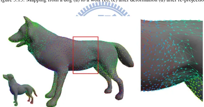
Notice that the deformation procedure can not guarantee that the deformed vertex lies ex-actly on the target surface. Therefore, we project the deformed base mesh to the nearest triangle of the target mesh to get the final mapping result. Figure 3.13 shows the result of the dog after the deformation and re-projection process. Since most of the hint positions of the inner ver-tices abide the convex combination constraint, the shape of the deformed source mesh usually close to the shape of the target mesh. Figure 3.14 and 3.15 shows the mapping vertices of the
3.5 Part boundary smoothing 29
dog model before and after the boundary smoothing process. We can observe that the map-ping positions of the vertices are nicely distributed along the part boundaries after the boundary smoothing process.
(a) (b) (c) (d)
Figure 3.13: Mapping from a dog (a) to a wolf (b), (c) after deformation (d) after re-projection.
Figure 3.14: Mapping vertices and edges of the dog model before part boundary smoothing (different edge color represents different parts).
3.5 Part boundary smoothing 30
Figure 3.15: Mapping vertices and edges of the dog model after part boundary smoothing (dif-ferent edge color represents dif(dif-ferent parts or the overlapping regions).
C H A P T E R
4
Experimental Result
In this chapter, we present the experimental result of the cross-parameterization with the pro-cessing time required, including cross-parameterization, part boundary smoothing, and repro-jection.
4.1
Result
In this section, we demonstrate the experimental result of our cross-parameterization method. The cross-parameterization between the two models is generated by minimizing the combi-nation error we proposed. Our method utilizes the skeleton-to-skeleton mapping and the dense skeleton-to-surface mapping to construct the cross-parameterization between two models. There-fore, we can generate the cross-parameterization for each pair of corresponding parts by speci-fying only two to three matching points on the part boundary such that part boundaries aligned on the parameterized domain. Figure 4.1 and Figure 4.2 shows the skeleton-to-surface mapping by coloring the surface with the same color of the correspondent skeleton node, which changes smoothly along the surface. The dense skeleton-to-surface mapping slices are shown in Figure
4.1 Result 32
4.3.
Figure 4.1: The visualization of skeleton-to-surface mapping of the dog model.
4.1 Result 33
Figure 4.3: The visualization of the skeleton-to-surface mapping slices.
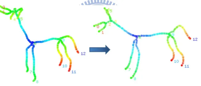
The skeleton-to-skeleton mapping is constructed by matching the junction and terminal skeleton node first. And the rest of the skeleton nodes are mapping through a linear interpola-tion along the skeleton path. Figure 4.4 shows the correspondence of the juncinterpola-tion and terminal skeleton node, each pair of the corresponding skeleton nodes are marked with same number. Figure 4.5 demonstrates the skeleton-to-skeleton mapping between the dog and wolf, we draw each skeleton node of the dog model with the mapping position on the skeleton path of the wolf model to visualize the skeleton-to-skeleton mapping.
4.1 Result 34
Figure 4.4: The skeleton node correspondence between the dog and wolf model
Figure 4.5: The skeleton-to-skeleton mapping between the dog and wolf model.
Figure 4.6 shows the matching points we assigned for each pair of parts The red colored edges are the part boundaries and the green colored edges represent the open boundaries which will be closed during the parameterization.
4.1 Result 35
Figure 4.6: The segmented parts and matching points colored in red and blue specified on the part boundaries.
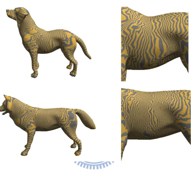
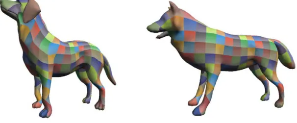
Since the proposed method measures the mapping error between two vertices by using the distance between their corresponding skeleton points along the skeleton. Therefore, the method can handle the cases in which models have feature parts in different orientations and size. Fig-ure 4.7 shows the cross-parameterization result between the dog and wolf, who have ears in extremely different orientation. We visualize the mapping results by texture mapping the target models with a check board texture.
4.1 Result 36
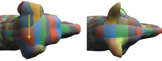
With the skeleton-to-skeleton mapping and the dense skeleton-to-surface mapping informa-tion, the object features between models can be matched automatically. To closely observe the mapping result for the local regions, we increase the texture repeat cycles and showed the re-sult in Figure 4.8, Figure 4.9, and Figure 4.10. Since the mapping error is defined only as the distance on the skeleton, some twists may happen along the direction which perpendicular to tangent of the skeleton due to the lack of the orientation information (as shown in the indicative region in Figure 4.10).
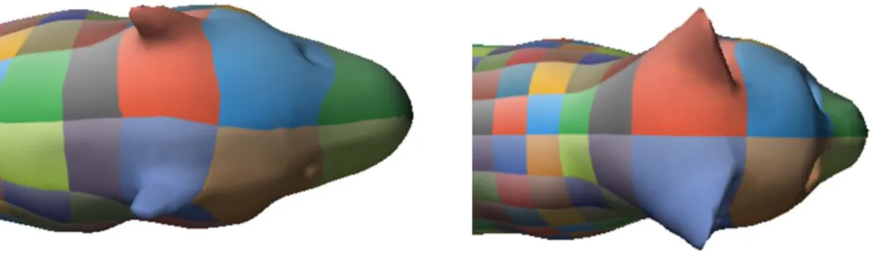
Figure 4.8: The cross-parameterization of the heads between the dog and wolf model.
(a) (b)
Figure 4.9: The cross-parameterize result of the limbs between the dog and wolf model. (a) front legs (b) back legs.
4.1 Result 37
Figure 4.10: The twist effect due to the lack of the orientation information on the slice region.
We also test our work on the lion and cat models with different size of parts, such as fore-head, ears, neck, limbs, belly, etc. As shown in Figure 4.11 - Figure 4.14, the lion has larger forehead and smaller ears than that of cat. Also, the length and the shapes of their limbs are different. Our method matches these features well without much distortion.
4.1 Result 38
Figure 4.12: The cross-parameterization of the head part between the lion and cat model.
Figure 4.13: The cross-parameterization of the front legs between the lion (top) and cat (bot-tom). The texture repeat cycle is doubled from left to right to clarify the result.
4.1 Result 39
Figure 4.14: The cross-parameterization of the back legs between the lion (top) and cat (bot-tom). The texture repeat cycle is doubled from left to right to clarify the result.
Since the vertices around the tip of an object part usually map to the same skeleton node, the mapping error of these vertices are the same. Therefore, it is hard to map the tip region well if the skeleton does not protrude close enough to the surface. As shown in the squared region in Figure 4.9 and Figure 4.15, the tip region of the left back leg maps to the same skeleton node and higher geometry distortion is induced in the tip area. Compare to mapping results of the front legs in Figure 4.13, we observe that the mapping results around the tip regions of the front legs are better than that of the back legs between the lion and the cat model. This is because the shape of the front legs between the lion and the cat are similar. In this situation, we can easily find the optimal cross-parameterization that minimizes the energy without much distortion. Thus the area around the tip region can be matched well automatically even when
4.1 Result 40
the skeleton does not protrude close enough to the surface.
Figure 4.15: The cross-parameterization and slicing of the skeleton-to-surface mapping of the left back leg of the lion and cat model.
(a) (b) (c)
Figure 4.16: The cross-parameterization of the front legs between the lion (top) and cat (bottom) model with different cut positions. (a) upper one-third (b) middle (c) lower one-third.
4.1 Result 41
In Figure 4.16, we show the mapping result for the parts resulting from different cutting po-sitions. The dotted lines represent the cutting positions in the segmentation process. We observe that inappropriate segmentation often results in cross-parameterization of higher distortions; as shown in the squared region. Since cut in these positions, one of the segment parts that shared the cut boundary is large and having higher stretch on the parameterize domain. As in Figure 4.16(c), cutting in the lower one-third of the legs makes the front belly of the lion and cat be-come much larger, and result in cross-parameterization of higher distortion compare to (a) and (b).
We also derived the cross-parameterization for the models in different poses. Since the object has similar topology, the cross-parameterization between them can be easily done with our approach. In Figure 4.17 - Figure 4.19 we demonstrate the cross-parameterization between the horse in the standing pose and in normal pose. We observe that our method is insensitive to the pose.
Figure 4.17: The cross-parameterization between the horse models in the standing pose and in normal pose.
4.1 Result 42
Figure 4.18: The cross-parameterization between the head parts of the horse model in different poses.
Figure 4.19: The cross-parameterization between the left front legs of the horse models in different poses.
4.1 Result 43
Next, we change the weight for the mapping error term to show its influence in the opti-mization process. To show the influence of the mapping error with different weights, we test the parts that have extremely different sizes and fineness. In the example, we enlarge the cat ears and do the subdivision such that the ear has four times number of faces as the lion’s ears. The cross-parameterization results with mapping error of different weights are shown in Figure 4.20. When the weight wm of the mapping error increases, we observe that the mapping area of
the cat’s eats lies closer to the place with lower mapping error. However, if the weight wmis too
high, the mapping area will suffer in high stretches and distortions on the target surface. Also, as shown in Figure 4.21, we observe a nearly opposite trend compares to Figure 4.20 when the influence of the stretch error increases.
wm= 1.0 wm= 1.5 wm= 2.0 wm= 2.5 wm= 0.5 ws = 1.0 (a) wm= 1.0 wm= 1.5 wm= 2.0 wm= 2.5 wm= 0.5 ws = 1.0 (b) wm= 1.0 wm= 1.5 wm= 2.0 wm= 2.5 wm= 0.5 ws = 1.0 (c) wm= 1.0 wm= 1.5 wm= 2.0 wm= 2.5 wm= 0.5 ws = 1.0 (d) wm= 1.0 wm= 1.5 wm= 2.0 wm= 2.5 wm= 0.5 ws = 1.0 (e)
Figure 4.20: The mapping result from a long ear cat head to the lion head with different mapping error weights.
4.1 Result 44 ws= 1.0 ws= 1.5 ws= 2.0 ws= 2.5 ws = 0.5 wm= 1.0 (a) ws= 1.0 ws= 1.5 ws= 2.0 ws= 2.5 ws = 0.5 wm= 1.0 (b) ws= 1.0 ws= 1.5 ws= 2.0 ws= 2.5 ws = 0.5 wm= 1.0 (c) ws= 1.0 ws= 1.5 ws= 2.0 ws= 2.5 ws = 0.5 wm= 1.0 (d) ws= 1.0 ws= 1.5 ws= 2.0 ws= 2.5 ws = 0.5 wm= 1.0 (e)
Figure 4.21: The mapping result from a long ear cat head to the lion head with different stretch error weights.
In general, we set wsa little bit higher than wmdue to our mapping error lacks the orientation
information. Setting wshigher can prevent the shape from distorting a lot during the relaxation
process (as shown in Figure 4.20 (e)). But when the size and fineness of the parts differs a lot, setting wmhigher than wsis necessary (as shown in Figure 4.20 (c)), since the high stretch error
constrain the vertex from moving further to the ideal position during the relaxation process. We also show the cross-parameterization between the parts with extremely different sizes and fineness. In Figure 4.22 - 4.24, we can observe that the ear parts still can approximately match to each other.
4.1 Result 45
Figure 4.22: The cross-parameterization between the long ear cat head and lion head (side view).
Figure 4.23: The cross-parameterization between the long ear cat head and lion head (front view).
4.1 Result 46
Figure 4.24: The cross-parameterization between the long ear cat head and lion head (top view).
If the mapping error is carefully tuned by the users during the mapping error relaxation, our method can be applied to the models which have extremely different appearance. User can tune the weight wmto be a little bit higher if the distance between the vertex and the reasonable
mapping positions are far after the relaxation. On the other hand, if user observes high distortion of the mapping polygons, user may lower the weight wm and let the weight wsto be higher. In
Figure 4.25 - Figure 4.29, we demonstrate an example of the cross-parameterization between the dragon and the wolf model. Since the shapes of the two models are extremely different, high distortion observed in these cases usually can not be avoided (as shown in Figure 4.30).
4.1 Result 47
Figure 4.25: The cross-parameterization between the dragon and wolf model.
Figure 4.26: The cross-parameterization of the head part between the dragon and the wolf model.
4.1 Result 48
(a) (b)
Figure 4.27: The cross-parameterization of the limbs between the dragon and wolf model. (a) right front leg (b) left front leg.
(a) (b)
Figure 4.28: The cross-parameterization of the limbs between dragon and wolf model. (a) right back leg (b) left back leg.
4.1 Result 49
Figure 4.29: The cross-parameterization of the tail part between the dragon and wolf model.
Figure 4.30: The visualization of slice mapping from the dragon to the wolf model.
4.1 Result 50
in Figure 4.31. Skeleton paths that linked by the matched skeleton nodes are corresponded accordingly. The mappings of the skeleton nodes inside the skeleton path are generated auto-matically through a linear interpolation along the skeleton path. For those nodes that do not have correspondences, their corresponding positions are the nearest node that has correspon-dence. For example, the three protrusions on the dragon’s tail will be corresponded to the skeleton node 12 of the wolf model. Therefore, the mapping of these unique feature parts will be constrained to the nearby area on the target model by minimizing both of the stretch and mapping error. Since the mapping error can only constrain the mapping position of the unique feature parts in nearby approximated regions, the qualities of the mapping still have room for improvement.
Figure 4.31: Skeleton node correspondence between the dragon and wolf model.