使用重疊球體正向模型以及階層搜尋光束構成進行腦電波訊號源定位

全文

(1)國立交通大學資訊工程學系碩士論文. 使用重疊球體正向模型以及階層搜尋光束構成進行腦電波訊號源定位 EEG Source Estimation using Overlapping-Sphere Forward Model and Hierarchical-Search Beamforming. 研究生：楊仲凱指導教授：陳永昇助理教授. 中華民國九十四年七月.

(2) EEG Source Estimation using Overlapping-Sphere Forward Model and Hierarchical-Search Beamforming. A dissertation presented by. Zhong-Kai Yang to. Department of Computer Science and Information Engineering in partial fulfillment of the requirements for the degree of Master of Science in the subject of. Computer Science and Information Engineering National Chiao Tung University Hsinchu, Taiwan 2005.

(3) EEG Source Estimation using Overlapping-Sphere Forward Model and Hierarchical-Search Beamforming. c 2005 Copyright by Zhong-Kai Yang.

(4)

(5) 學生：楊仲凱. 指導教授：陳永昇. 國立交通大學資訊工程研究所碩士班摘. 要. 腦，是人體當中最重要且複雜的器官，對於腦功能的探索，是目前最熱門的研究課題之一。腦電波儀是常被用來進行腦功能研究的工具之一，因為它具有相當高的取樣頻率以及低廉的價位。在本篇論文中，我們將會提出一個準確且快速的腦電波訊號源定位方法，包括了正向模型的計算（針對已知的訊號源計算腦電波），以及如何去解決反向問題（利用腦電波來進行訊號源定位）。在所提出的正向模型中，我們針對每個腦電波儀感應器找出適合的重疊球體，以增加正向模型的準確度。並且，重疊球體只需要使用多層球體結構即可很快速的計算出來，而不需要去計算相當耗時的邊界元素模型。基於所提出的正向模型，我們使用階層搜尋光束構成來解決反向問題。經由最大化腦電波的活動狀態和控制狀態的強度對比，可以大幅地增加訊號源定位結果的準確度。並且，在腦空間中搜尋訊號源時我們使用階層搜尋而非全域搜尋，亦能有效地降低解決反向問題的時間。根據假體實驗以及視覺刺激實驗結果，確認了我們所提出的方法之準確性以及便利性。我們所提出的訊號源定位法可以有效地被使用在無需磁振造影資料的情形，例如進行基礎腦科學的研究，或者腦機介面的開發。.

(6) Abstract. Brain is the most important and complicated apparatus of human beings. EEG has been widely applied in functional brain studies due to its high temporal resolution and low cost. In this work, we focus on the development of an accurate and efficient EEG forward model as well as the inverse solution for neuronal source estimation from the EEG measurements. Our forward model successfully gains its accuracy by fitting an overlapping sphere for each EEG sensor. The computation of the overlapping sphere requires only the multi-shell geometry, instead of boundary element method, thus the proposed forward model is easy to compute. Based on the proposed forward model, the beamforming technique is applied to calculate the distributed sources in the brain space. We maximize the power contrast between active state and control state of EEG recorded data to improve the accuracy of inverse solution. Hierarchical search in the solution space is applied to save the amount of computation by searching grid point level by level instead of searching the whole brain space. According to our experiments using phantom data and visual-evoked potential data, the proposed forward model and inverse solution can efficiently and accurately estimate the source of brain activation. A quick and reliable source localization technique for EEG is successfully developed which can be applied on applications when MRI is not available, such as fundamental brain research and brain-computer interface.. i.

(7) 誌. 謝. 短短的二年碩士生涯即將結束，在這二年當中，首先要感謝及. 陳永昇老師以. 陳麗芬老師帶領我踏入生醫訊號處理的領域，並提供完善且齊備的資源、設. 備讓初次進行腦科學研究的我，能夠快速地學習到許多專業技能；並且在為人處世上也常啟迪我許多做人做事的道理，這些都將成為我將來進入社會工作莫大的助力。其次要感謝口試委員. 謝仁俊醫師，在口試當中所給予我的專業意見，對. 於我的研究有很大的助益；在此致上最誠摯的謝意。二年的研究生涯當中，實驗室的同學們給予了我莫大的幫助以及鼓勵。嘉修學長常在會議中提出過來人的見解，讓我了解自己看不見的缺失。安廷、福慧常陪伴我運動，每當我在研究遇上瓶頸時，你們總是能讓我忘卻煩惱。志瑜相當認真於專業領域的研究，是我在實驗室中的榜樣。同窗好友昭翰、怡岑總是笑臉迎人，是我心情不佳時最好的聊天對象。當然還有二位可愛的學妹盈盈、承嘉，以及三位搞笑的學弟政毅、凱為、聖翰，實驗室只要有你們在，總是會不斷地傳出笑聲；和大家去宜蘭童玩節遊玩的回憶真的是相當開心。最後感謝從小到大辛苦栽培我的父母，沒有你們多年來的教誨，也不會有今天的我。還有長久以來總是支持我的凡毓，你對我的支持就是我繼續前進的動力。二年的研究所學業絕對不是我能夠一力完成的，再次由衷地感謝所有曾經幫助過我的親友、師長、同學們。仲凱. 2005.7.31.

(8) Contents List of Figures. v. List of Tables. vii. 1. Introduction 1.1 Background . . . . . . . . . . . . . . . . . . . . . . . . . . . . . . . . . . 1.2 Thesis scope . . . . . . . . . . . . . . . . . . . . . . . . . . . . . . . . . . 1.3 Organization of this thesis . . . . . . . . . . . . . . . . . . . . . . . . . .. 2. Forward Model 2.1 Previous works . . . . . . . . . . . . . . . 2.1.1 Single-shell model . . . . . . . . . 2.1.2 Multi-shell model . . . . . . . . . . 2.1.3 Boundary element model . . . . . . 2.2 Proposed method . . . . . . . . . . . . . . 2.2.1 Background of overlapping spheres 2.2.2 Calculation of overlapping spheres . 2.2.3 Calculation of inner skull surface . 2.2.4 Correction of overlapping spheres .. 3. 4. Inverse Problem 3.1 Previous works . . . . . . . . . . . . . . 3.1.1 Fitting method . . . . . . . . . . 3.1.2 Scanning method . . . . . . . . . 3.2 Proposed inverse solution . . . . . . . . . 3.2.1 Maximum contrast Beamforming 3.2.2 Hierarchical-Search Beamforming. . . . . . .. . . . . . . . . .. . . . . . .. . . . . . . . . .. . . . . . .. . . . . . . . . .. . . . . . .. . . . . . . . . .. . . . . . .. . . . . . . . . .. . . . . . .. . . . . . . . . .. . . . . . .. . . . . . . . . .. . . . . . .. . . . . . . . . .. . . . . . .. . . . . . . . . .. . . . . . .. . . . . . . . . .. . . . . . .. . . . . . . . . .. . . . . . .. . . . . . . . . .. . . . . . .. . . . . . . . . .. . . . . . .. . . . . . . . . .. . . . . . .. . . . . . . . . .. . . . . . .. . . . . . . . . .. . . . . . .. 1 2 4 5. . . . . . . . . .. 7 8 8 9 13 13 13 15 18 19. . . . . . .. 21 22 22 24 28 28 29. Experiments 33 4.1 Phantom data . . . . . . . . . . . . . . . . . . . . . . . . . . . . . . . . . 34 4.1.1 Comparison between forward models . . . . . . . . . . . . . . . . 34 4.1.2 Inverse accuracy verification . . . . . . . . . . . . . . . . . . . . . 36 iii.

(9) 4.2 5. Real experiment . . . . . . . . . . . . . . . . . . . . . . . . . . . . . . . . 39. Conclusions. 45. Bibliography. 47. iv.

(10) List of Figures 1.1 1.2 1.3 1.4. EEG can sense the radial oriented brain activities. . . . Open and closed fields. . . . . . . . . . . . . . . . . . Various source models. . . . . . . . . . . . . . . . . . Flowchart of the forward model and inverse estimation.. 2.1 2.2 2.3 2.4. 2.6 2.7 2.8. Single-shell model diagram with current dipole. . . . . . . . . . . . . . . Multi-shell (four-shell) model diagram. . . . . . . . . . . . . . . . . . . The concept of Berg method. . . . . . . . . . . . . . . . . . . . . . . . . Values of cn f n−1 with respect to n for the four-shell model of Cuffin and Cohen. . . . . . . . . . . . . . . . . . . . . . . . . . . . . . . . . . . . . Comparison between the best-fitted sphere model and the overlappingsphere model . . . . . . . . . . . . . . . . . . . . . . . . . . . . . . . . Flowchart of the proposed OS forward model. . . . . . . . . . . . . . . . An illustration of mapping realistic mesh points to approximated sphere. . Flowchart of overlapping sphere procedure. . . . . . . . . . . . . . . . .. 3.1 3.2 3.3. Beamforming example : Airplane & radar. . . . . . . . . . . . . . . . . . . 25 Flowchart of beamforming method. . . . . . . . . . . . . . . . . . . . . . 30 Two cases that brain source is outside sphere model. . . . . . . . . . . . . . 31. 4.1 4.2 4.3 4.4 4.5 4.6 4.7 4.8. X-ray projection of the skull phantom and EEG electrodes. . . . . . . . . Flowchart of the correctness verification on forward and inverse method. . Correlation comparison between Berg method and Sun method. . . . . . Snapshot of forward comparison topography with dipole #20. . . . . . . . Slice-view of two brain activation results. . . . . . . . . . . . . . . . . . Source localization error comparison between our method and EEGLAB. VEP comparison between beamforming and dipole-fitting results. . . . . AEP comparison between beamforming and dipole-fitting results. . . . .. 2.5. v. . . . .. . . . .. . . . .. . . . .. . . . .. . . . .. . . . .. . . . .. . . . .. . . . .. . . . .. 2 4 5 6. . 8 . 10 . 11 . 12 . . . .. . . . . . . . .. 14 15 17 19. 34 35 37 38 40 41 42 43.

(11) vi.

(12) List of Tables 4.1 4.2. Averaged correlation comparison between various forward models. . . . . . 36 Localization error of various forward models and inverse estimation methods. 39. vii.

(13) viii.

(14) Chapter 1 Introduction.

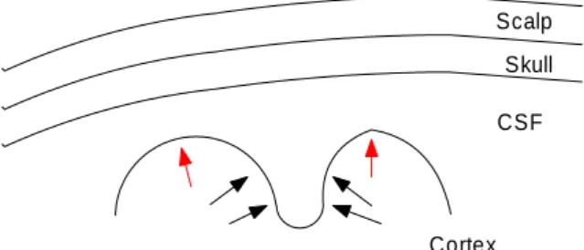
(15) 2. Introduction. Scalp Skull CSF. Cortex. Figure 1.1: EEG has some advantages than MEG, such as it can sense the radial oriented brain activities (red arrows).. 1.1. Background. Brain, like the CPU (Central Process Unit) of computer, is the central controller of human body. It is the unique and most important apparatus of human beings that controls all of the human activities, such as muscle movement, action reaction, our feeling of something, the emotion, and so on. Brain is also the most complicated apparatus of our body. To understand what our brain does we can use several noninvasive functional brain imaging tools such as EEG (ElectroEncephaloGraphy), MEG (MagnetoEncephaloGraphy), and fMRI (functional Magnetic Resonance Imaging) to help us unravel dynamics of cortical function. EEG records the electric potential on the scalp surface produced by the neural activation using its electrodes attached on the scalp. MEG record the magnetic field produced by neural currents by the array of superconductive sensors [10]. fMRI provides a method of visualizing a correlate of neural activity in the human brain [26]. EEG is a recording (graph) of electric signals (electro) from the brain (encephalo). It has sensors that can measure electric potential on scalp surface. In 1929, H. Berger first published EEG of human beings. He successfully distinguish the β waves (13–35 Hz) by EEG signal. EEG / MEG have high sampling rate (temporal resolution) that can reach 1000Hz. Besides, EEG has some advantages compared with MEG, for example, EEG is more portable than MEG because EEG does not need shielding-room when sensing head surface potential. And, EEG can sense the brain activities with radial orientation to the scalp surface but MEG can not do this (See Figure 1.1)..

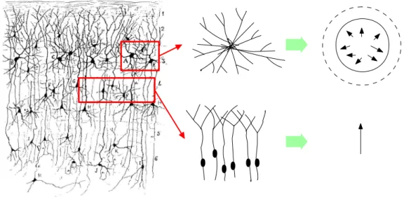
(16) 1.1 Background. The recorded EEG data can be used in many applications. For example, we can apply the “source localization” technique (to localize the neural activitives in the brain using EEG / MEG recorded data, also called “source estimation”) to determine the brain neural source. In clinical application, we can measure EEG of the epileptic patients and penetrate the disease focus and cortical dynamics using “source localization” technique. Or, we can extend “source localization” on the fundamental brain research and brain-computer interface systems. After the event-related potential (ERP) method is widely applied, scientists have great advancement in discovering brain activity from EEG. When giving a specific stimulus on nervous system, the induced surface potential variance is called ERP. For example, if we give the subject light, sound, or electrical stimuli, evoked surface potential can be extracted from EEG measured data. ERP component in EEG data is much smaller than noise component; we can generally assume that noise of each EEG sensor is zero mean, such that SNR (Signal-to-Noise Ratio) can be improved by applying synchronized averaging on EEG measured data. In reality, brain functions are the networks of many neural activities. Figure 1.2 shows “open field” (top part) and “closed field” (bottom part) concepts of neural activities. The principle cortical neurons are the pyramidal cells (left-most part, transverse section through the gray matter of rat cortex). Their apical dendrites from above reach out parallel to each other, so that they tend to be perpendicular to the cortical surface (open field) [11]. So they can be macroscopically modeled as some source model (bottom part). Besides, pyramidal cells connecting together may cancel out their current influences each other (top part, closed field). From above we know that actually characterizing all the neural activation in detail is difficult. We can macroscopically model the behavior of neural activation as many source models such as infinite cylindrical source, dipolar source, and octupolar source (Figure 1.3). ECD (Equivalent Current Dipole) form is proved as a better assumption of source modeling. Given a current dipole, the forward model can be used to calculate the scalp potential induced by this dipole source. On the other hand, the inverse problem is about how to estimate the brain activation from the scalp potentials recorded by EEG. Accuracy of inverse. 3.

(17) 4. Introduction. Figure 1.2: Difference between open field and closed field. Left-most part shows the transverse section through the gray matter of rat cortex drawn by Ramon y Cajal in 1888. The principle cortical neurons are the pyramidal cells, and their apical dendrites from above reach out parallel to each other so that they tend to be perpendicular to the cortical surface (open field). They can be equivalently modeled as some source model (bottom part). Besides, pyramidal cells connecting together may cancel out their current influences each other (top part, closed field).. problem is influenced by the accuracy of forward model, the SNR of EEG recording data, and the inverse methodology. If the source number is known a priori, least-square estimation can solve the inverse problem by fitting the potential field predicted by the forward model to the EEG recordings. Alternatively, distributed source estimation methods impose various kinds of constraints and obtain the neuronal activities for all the probed area in the brain. Figure 1.4 shows the flowchart of forward model and inverse problem estimation.. 1.2. Thesis scope. In this thesis, we propose a accurate and efficient EEG source estimation technique including forward model and inverse solution. In our new forward model, we use multi-spheres as head model and apply the overlapping spheres (OS) technique to improve the accuracy of forward model. The proposed.

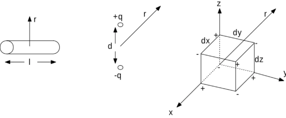
(18) 1.3 Organization of this thesis. 5. z +q. r. r. r dx. d. +. dy. -. +. -. -. l -q. dz +. +. y. -. x. Figure 1.3: Comparison of various source models. Left figure is infinite cylindrical source, center figure is dipolar source, and right figure is octupolar source. Dipolar source is proved as the best way to model neural activation.. forward model has following benefits: 1) Efficient calculation of surface potential by using a simplified formula. 2) Better accuracy by using the OS. 3) Easier calculation of the OS by using the multi-shell geometry instead of using the boundary element method (BEM) model. We also propose a new inverse estimation method, named hierarchical-search beamforming. This new inverse method has the following benefits: 1) A closed-form solution of the dipole source orientation. 2) Less tendency to trap into local optimum. 3) Efficient search by using the hierarchical framework.. 1.3. Organization of this thesis. In Chapter 2 we describe our forward model including previous works (Berg method and Sun method) and proposed OS technique. Solutions of inverse problem including.

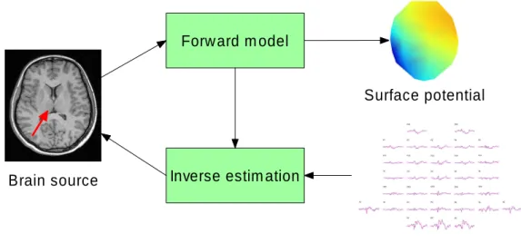
(19) 6. Introduction. Forward m odel Surface potential. Brain source. Inverse estim ation. EEG m easured data. Figure 1.4: Flowchart of the forward model and the inverse estimation. The forward model can calculate the surface potential using known current dipole, and the inverse estimation can estimate the current dipole using known surface potential.. fitting method and scanning method are described in Chapter 3. In Chapter 4 we introduce the experiment result applying our forward model and inverse method on phantom data and visual-evoked potential data. Finally, conclusions for our method and the relative results are described in Chapter 5..

(20) Chapter 2 Forward Model.

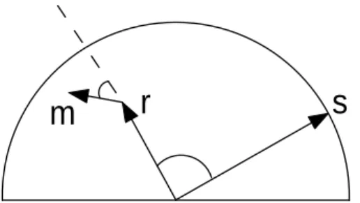
(21) 8. Forward Model. m. r. s. Figure 2.1: Single-shell geometry. Surface potential is measured at s where dipole located at r with m as moment (orientation and magnitude). The angle between vectors pointing to s and r is denoted θ. The angle the dipole moment m makes with the radial direction at r is denoted α, and β is the angle between the plane formed by r and m, and the plane formed by r and s.. In this section, we first briefly describe the previously-proposed forward models that are related to the proposed one. Then we will introduce the proposed forward model using the OS.. 2.1. Previous works. 2.1.1. Single-shell model. Although the real human brain is complicated which include cortex (gray matter and white matter), cerebrospinal fluid (CSF), skull, and scalp, we simply assume the head model as a sphere with homogeneous conductivity. By this assumption, we can calculate the forward model in a very simple way but does not guarantee the accuracy. In this section we introduce this easy and simple forward model. Before calculating the surface potential based on the single-shell head model, we need some pre-work. First, calculate a best-fit sphere among all the sensor locations. Use the least-square estimation to find out the best-fit sphere among all EEG sensors. Then, map the sensor locations onto the best-fit sphere surface such that we can estimate the surface potential (or leadfield) of the mapped sensor locations. The surface potential V 1 (s; r, m) at the sensor location s for a given dipole located at r and with m as the moment (See Figure 2.1), can be expressed as the sum of its radial.

(22) 2.1 Previous works. 9. Vr1 (s; r, m) and tangential Vt1 (s; r, m) surface component [20]: Vr1 (s; r, m) = ( Vt1 (s; r, m) = (. 1 1 mr 2(s cos θ − r) )( − ) + 3 4πσ d rd sr. 2s mt d+s ) cos β sin θ( 3 + ) 4πσ d sd(s − r cos θ + d). V 1 (s; r, m) = Vr1 (s; r, m) + Vt1 (s; r, m). (2.1). where d = s − r, s = ksk, r = krk, m = kmk, d = kdk, mr = m cos α, mt = m sin α, σ is the conductivity of this media, α is the angle between r and m, θ is the angle between s and r, and β is the angle between the plane formed by r and m, and the plane formed by r and s. Single-shell forward model is the simplest forward model, but contrarily it may cause large error because our head is not just a homogeneous sphere. To improve the accuracy of forward model, we have other assumptions like multi-shell model (Section 2.1.2) and BEM (Section 2.1.3) to approximate our human head geometry.. 2.1.2. Multi-shell model. Consider the fact that the human head consists of several kinds of tissues, such as scalp, skin, skull, cortex, and CSF. Different tissues have different conductivities. It will be more accurate to model the head as multiple concentric spheres. The conductivity is homogeneous in the volume between consecutive layers. In this work, we use four concentric spheres to model the following tissues: scalp, skull, cortex, and CSF. Based on the multipleshell spherical head model, we can calculate the scalp potential V M at sensor location s induced by the dipole source at position r and with orientation m [5, 24]:. V. with. M. ∞ X Pn1 (cos θ) 1 n−1 c f m· (r P (cos θ) + t ) (s; r, m) = n 0 n 0 4πσ4 R2 n=1 n. (2.2).

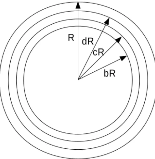
(23) 10. Forward Model. R dR cR bR. Figure 2.2: Central cross-section of the multi-shell (four shell) model. The brain, CSF, skull, and scalp regions are shown, and their respective conductivity values are labeled by σ1 , σ2 , σ3 , σ4 . The outmost boundary of these four shells are bR, cR, dR, R.. cn =. (2n + 1)4 (cd)2n+1 Γ. σ1 σ2 σ1 σ2 − 1)( − 1)(n + 1) + c2n+1 ( n + n + 1)( n + n + 1)) σ2 σ3 σ2 σ3 σ3 σ3 · (( n + n + 1) + (n + 1)( − 1)d2n+1 ) σ4 σ4 σ σ σ σ1 σ2 1 2 2 +(n + 1)c2n+1 (b2n+1 ( − 1)( n + + n) + c2n+1 ( n + n + 1)( − 1)) σ2 σ3 σ3 σ2 σ3 σ3 σ3 σ3 + n)d2n+1 ) · (n( − 1) + ( n + σ4 σ4 σ4 where R = ksk, f = krk/R, r0 and t0 are the radial and tangential unit vectors, respecΓ = d2n+1 (b2n+1 n(. tively, θ denote the angle between r and s, and Pn and Pn1 are the Legendre and associated Legendre polynomials of degree n, respectively. Multi-shell geometry is defined as Figure 2.2. Notice that in Equation (2.2) we need to calculate the recursive Legendre and associated Legendre polynomials which cost much time. Typically, the summation term will be converged after 200 to 300 iterations, which make this method inefficient. So this direct method is really an inefficient method..

(24) 2.1 Previous works. 11. Figure 2.3: In Berg method, a single source in a multi-shell model (left figure) can be well approximated by three sources in a homogeneous sphere model (right figure) [1, 29].. P. Berg, et al. [1, 29] and Mingui Sun [25] have introduced two different ways to enhance the efficiency of multi-shell forward model. Following we describe how these two methods work. Berg method In [1], P. Berg and M. Scherg presented an efficient way to calculate the forward model based on multi-shell spherical head model. This method uses the true dipole location r to select three dipole locations along the same radial line, and calculate these surface potentials using single-shell model (Equation (2.1)) three times (Figure 2.3). The surface potential of multi-shell model using Berg’s method will be approximated as. V M (s; r, m) ∼ = V 1 (s; µ1 r, λ1 m) + V 1 (s; µ2 r, λ2 m) + V 1 (s; µ3 r, λ3 m). (2.3). where µi and λi (i = 1,2,3) are called “Berg Parameters” which are only related to the head conductivities and shell thickness such that can be predetermined to save the calculation time. See [29] for details of “Berg Parameters” computation according to the head geometry. In this method, infinite summation term in Equation (2.2) for a single dipole using the multiple-shell spherical head model can then be replaced by a summation of these three.

(25) 12. Forward Model. Figure 2.4: Values of cn f n−1 with respect to n (solid line, f = 0.85) for the four shell P model of Cuffin and Cohen [5]. The polynomial fitting, 3k=0 ak nk f n−1 is plotted as cross patterns. The circular patterns denote the original values. It’s clear that the fitting (cross patterns) is very close to the real values (solid line). (Figure source: [25].). dipoles using the single-shell spherical head model. Because of above event, using Berg method will let multi-shell model faster. Sun method Another approximation method based on multi-shell model was introduced by Mingui Sun [25]. The main concept of Sun’s method is to use a polynomial function, whose calculation is more efficient, to approximate the summation term in Equation (2.2). Figure 2.4 shows a curve of cn f n−1 (solid line) used in Equation (2.2). Notice that excepting for first few values (n < 5), remaining values tend to follow a smooth v-shaped curve. In Sun method, the infinite summation term in Equation (2.2) can be separated into two parts. The first part involves the first N terms (often takes N = 3) using exact values (circular patterns). The second part is composed of the remaining terms of the infinite summation which will be approximated by a closed-form formula (cross patterns). Following is the refined equation: V M (s; r, m) =. ∞ X Pn1 (cos θ) 1 n−1 c f m· (r P (cos θ) + t ) n 0 n 0 4πσ4 R2 n=1 n.

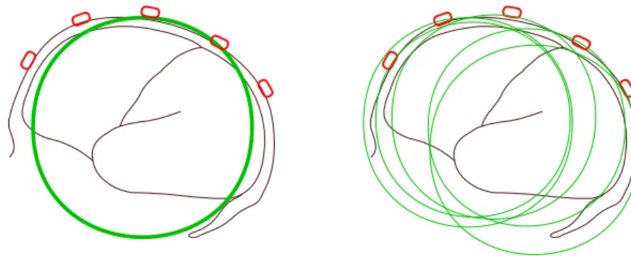
(26) 2.2 Proposed method. ∼ =. 13. N X. cn f. n−1. Qn +. n=1. ∞ X. (. K X. ak nk )f n−1 Qn. (2.4). n=N +1 k=0. where Qn =. 1 Pn1 (cos θ) ). m· (r P (cos θ) + t 0 n 0 4πσ4 R2 n. See [25] for details of how to compute the closed form formula. PK. k=0. ak nk . It has. shown that the best selection of N and K is N = K = 3. Furthermore, a C-code program of evaluating the surface potential at sensor location s for a known dipole location r and orientation m was also presented in [25]. Both of the Berg and Sun’s methods improve the efficiency of forward calculation at the expense of losing some accuracy. More detailed comparison between Berg method and Sun method is described in Chapters 4 and 5.. 2.1.3. Boundary element model. BEM model is the most realistic head model because it uses the triangle meshes to separate tissues with different conductivities, such as brain, skull, and scalp. Conductivity can then be well set throughout the head. However, calculation of BEM model is timeconsuming and the head MRI (Magnetic Resonance Imaging) of the subject is required to reconstruct the tissue surfaces.. 2.2 2.2.1. Proposed method Background of overlapping spheres. There is a problem in using the spherical-based forward model, as shown in Figure 2.5. Because EEG sensors are attached on the scalp surface, which is not a perfect sphere, there will be deviation from the EEG sensor to the surface of the spherical model. The farther EEG sensor is from the sphere surface, the larger error of the estimated surface potential.

(27) 14. Forward Model. Figure 2.5: (Left) Calculation for a single best-fitted sphere is simple, but the sensors are deviated from the spherical surface. (Right) Using a sensor-fitted sphere for each sensor can improve the forward model accuracy.. for this sensor will has. In this section, we reform this drawback to reduce the error of multi-shell based forward model. One remedy is to use the sensor-fitted spheres, also called overlapping spheres, for each sensor instead of using only one best-fit single-sphere for all sensors. Mosher et al. presented the idea of applying OS for MEG in [13], and then extended its application to EEG in their following work [7]. Their method calculates the OS by minimizing the difference of leadfields between BEM and multiple-shell spherical forward model using the approximated OS as the head model:. {R0 , C0 } = arg min (kgsph (s, r, σ, ρR0 ) − gBEM (s, r, σ)k) R0 ,C0. (2.5). where σ = {σ1 , σ2 , σ3 , σ4 } indicates layer conductivities; ρR0 = {ρ1 R0 , ρ2 R0 , ρ3 R0 , ρ4 R0 } is sphere radii with assumed fixed relative ratio ρi (i = 1, . . . ,4). R0 and C0 denote sphere radius and center, and gsph and gBEM are the leadfield vectors for the spherical and BEM solutions respectively. In this method (OS applied to EEG), we found that BEM leadfield was required to calculate OS, but we know that calculating BEM leadfield is timeconsuming (Section 2.1.3). And, a significant number of BEM leadfield evaluations are also required to evaluate the obtained OS.

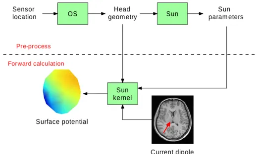
(28) 2.2 Proposed method. Sensor location. 15. OS. Head geom etry. Sun. Sun param eters. Pre-process Forward calculation. Sun kernel. Surface potential. Current dipole. Figure 2.6: Flowchart of the proposed OS forward model. (Top) Pre-processing procedure, including OS and Sun’s parameters calculation, can be performed beforehand. (Bottom) calculation of surface potential using Sun’s parameters.. 2.2.2. Calculation of overlapping spheres. In this work, we develop a new calculation method for OS without calculating the timeconsuming BEM model. The proposed method uses the multiple-shell geometry, instead of the BEM model, to estimate the OS. Thus the computation of the proposed method is much more efficient than that proposed in [13]. Figure 2.6 shows the flowchart of the proposed OS method for forward model calculation. Top part containing procedures of OS and Sun parameters producing. Both of them can be estimated before actually estimating surface potential. Bottom part is the forward model calculation which estimates surface potential. In Section 2.2.2, detail of calculating OS is presented; Sections 2.2.3 and 2.2.4 shows other required estimations and correction of OS. Assume that the human head has m layers and denote the surfaces between tissues with different conductivities as S1 ,S2 ,. . . ,Sm . The surface potential V (s) of the sensor location s on the jth surface can be estimated by the second kind Fredholm integral [8]:.

(29) 16. Forward Model. m s−r 1 X σi− − σi+ Z 2σm V (r)n(r)· V (s) = − dSi0 + V∞ (s) − + − 3 σj + σj 2π i=1 σi + σi Si ks − rk. s ∈ Si. (2.6). with 1 Z p s−r V∞ (s) = j (r)· dv 0 3 4πσm G ks − rk. (2.7). where σi− and σi+ are the conductivities inside / outside the ith surface, respectively, jp (r) is the primary current, and n(r)dSi0 is a vector element of surface Si with its direction aligned to outward surface normal of the surface Si . Primary current is unrelated to the spherical geometry and can be dropped. Therefore we can calculate the OS by fitting the return current contribution term in Equation (2.6) based on the spherical model: Z jfsp (r) jfre (r) s − rre s − rsp 0 0 ∼ sp (n (r)· ( re (n (r)· ) − ) − + dSi − + dSi ) = 0 sp re 3 sp 3 ks − r k σi + σi ks − r k σi + σi Si i=1 Si (2.8). m Z X. re. where the superscript re stands for the realistic head, sp stands for the approximated head, and jf (r) is the secondary current on each surface: jf (r) = −(σi− − σi+ )V (r)n(r) = jf (r)n(r).. (2.9). Human skull conductivity is about two orders of magnitude less than the other tissue conductivities, such as brain and scalp. Therefore, the dominant return current contributions will come from the innermost skull [12]. Thus, we can simply evaluate the integral on the innermost skull surface. It has been shown that true potentials and spherical potentials are not dramatically different [13], so we simply assume jfre = jfsp and rewrite Equations (2.8) and (2.9) as: Z re Sinnerskull. (nre (r)·. s − rre s − rsp sp − n (r)· )j re (r)dS 0 ∼ = 0. ks − rre k3 ks − rsp k3 f. (2.10).

(30) 2.2 Proposed method. 17 rre(i). rsp(i) R0 (0,0,0). C0. Figure 2.7: An illustration of mapping realistic mesh points (rre (i) and nre (i)) to approximated sphere. Thus, we can express rsp (i) and nsp (i) in terms of rre (i) and nre (i) (See Equations (2.12) and (2.13)).. To solve Equation (2.10) we use two dense surface meshes containing N points to represent the realistic innermost skull surface and the fitting sphere, respectively. The leastsquare fitting problem is simply to minimize the following equation (cost function): N X. knre (i)·. i=1. s − rsp (i) 2 s − rre (i) sp − n (i)· k ks − rre (i)k3 ks − rsp (i)k3. (2.11). where rre (i) and nre (i) (i = 1, 2, . . . , N ) denote the locations and normal orientations of the mesh points on the innermost skull surface, respectively, and rsp (i) and nsp (i) are those for the approximating sphere. Given a sphere {C0 , R0 }, rsp (i) can be obtained by radially mapping rre (i) to the surface of the approximated sphere. Thus we can substitute expressions for rsp (i) and nsp (i) in terms of the rre (i) and nre (i) as rsp (i) = R0 (. and. rre (i) − C0 ) + C0 krre (i) − C0 k. (2.12).

(31) 18. Forward Model. nsp (i) =. rre (i) − C0 . krre (i) − C0 k. (2.13). Therefore, Equation (2.11) can be written as the final cost function: re. (i)−C0 ) 2 s − C0 − R0 ( krrre (i)−C s − rre (i) rre (i) − C0 0k re min kn (i)· k. · − re (i)−C0 3 R0 ,C0 ks − rre (i)k3 krre (i) − C0 k ks − C0 − R0 ( krrre (i)−C )k i=1 k 0 (2.14) N X. To solve this non-linear optimization problem, we use the widely-used simplex method – Nelder-Mead method presented in [22]. For each EEG sensor, a sphere can be yield by applied Equation (2.14). Repeating Equation (2.14) for each EEG sensor yields a set of overlapping spheres.. 2.2.3. Calculation of inner skull surface. Equation (2.14) needs the realistic parameters: rre (i) and nre (i) (i = 1,2,. . . ,N ). Now we show how to estimate them using given EEG sensor locations s(i) (i = 1,2,. . . ,N ). Assume vertex i is surrounded with M triangles whose normals are n1 , n2 , . . . , nM and superficial measures are a1 , a2 , . . . , aM (evaluated by Heron’s formula), respectively. nre (i) can be estimated by: PM. n (i) =. aj nj . j=1 aj nj k. j=1. re. k. PM. (2.15). Assume that the thickness of scalp and skull is constant throughout the human head. rre (i) can be estimated by: rre (i) = s(i) − T nre (i). (2.16). where s(i) is the i-th sensor location, and T denote the average thickness of human scalp and skull [17, 19]..

(32) 2.2 Proposed method. 19. Sensor location s(i). Corrected OS R 0 , C' 0. OS correction (Equation 2.17). Equation 2.15 and 2.16. Realistic innerskull nre (i), rre (i). OS cost function (Equation 2.14). OS R 0 , C 0. Figure 2.8: Flowchart of OS parameter calculation. First, we find inner skull normals nre (i) and mesh locations rre (i). Second, Equation (2.14) is used to evaluate the OS radius R0 and center C0 . Finally, we can correct the estimated OS to fit EEG sensor location to the OS boundary.. 2.2.4. Correction of overlapping spheres. The calculated OS boundary of each sensor may not perfectly fit the sensor locations because of the non-linear search procedure in Equation (2.14). Two simple ways can be used to adjust the OS to fit to each EEG sensor location: 1) to translate the sphere center, and 2) to change the sphere radius. By the test on phantom data in Chapter 4, we find that “Translate the sphere center” performs better than the other correction method. We use following equation to translate sphere center to fit OS boundary and EEG sensor: C00 = s(i) + (. R0 )(C0 − s(i)) kC0 − s(i)k. (2.17). for ith sensor (i = 1,2,. . . ,N ). Figure 2.8 shows the flowchart of the proposed OS forward model. First, we use Heron’s formula and the weighted normal to find the inner skull normals nre (i) and evaluate inner skull mesh locations rre (i) by assuming that the thickness of scalp and skull is constant. Then, the OS cost function described in Equation (2.14) is applied to estimate the sphere radius R0 centered at C0 . Finally, we can correct estimated OS by translating its sphere center C0 to fit the EEG sensor to the OS boundary..

(33) 20. Forward Model.

(34) Chapter 3 Inverse Problem.

(35) 22. Inverse Problem. In this chapter, we start to solve the ”inverse problem.” That is, we want to estimate the neural activation using known measured surface potential. Before solving the inverse problem, a good forward model is needed. Using a good forward model, the relative inverse solution will be accurate; on the other hand, the inverse solution will be inaccurate if the forward model is not good enough. Inverse problem is an ill-condition problem which may result in variable solutions. Because of this property, we cannot precisely find a closed-form solution of inverse problem. In Section 3.1, the non-linear optimization method is applied to solve this. There are several widely-used non-linear method can be used, such as Nelder-Mead method, Powell method, and Levenberg-Marquardt method [22]. The same as Section 2.2.2 (Equation (2.14)), we select Nelder-Mead method as the non-linear optimization method. Another method to solve ill-condition problem is applying the global-search (gridsearch) method. Solution based on global-search won’t trap into local minimum where non-linear optimization will, but it costs much more time than using non-linear optimization. In Section 3.2, we develop a hierarchical grid-search based method. This new method still preserve the advantage of grid-search based method (won’t trap into local minimum), and, it will cost less time than global-search method.. 3.1. Previous works. Inverse solution can be separated as fitting method and scanning method. Fitting method including focal source and distributed source solves inverse problem by fitting the measured surface potential to the predicted surface potential from the EEG forward model. Scanning method is to scan the whole brain space and reveal locations having significant neuronal activation.. 3.1.1. Fitting method. Here we find the inverse solution by fitting our predicted surface potential and EEG measured surface potential. The source can be focal source or distributed source. Focal source, so-called dipole source, including single dipole and multiple dipoles needs source.

(36) 3.1 Previous works. 23. number as prior knowledge while distributed source does not. Distributed source assumption is obviously more reasonable, but the focal source assumption can quickly indicate where the area neural activation is. Focal source Least-square estimation Assume brain source consists of only a single dipole. Leastsquare estimation can be used to solve the inverse problem. Assume the EEG equipment has N sensors, x is a vector with N dimension which contains the EEG measured data. Following steps are the algorithm of least-square estimation: 1) For a given initial guess current dipole located at r0 and known EEG sensor locations, use forward model presented in Chapter 2 to calculate the leadfield GN ×3 . 2) Use SVD (Singular Value Decomposition) method [22] to estimate the dipole moment q = G−1 x. 3) Calculate the predicted potential x0 = Gq. 4) Use the non-linear optimization method to solve minkx − x0 k = minkx − G(G−1 x)k. 5) Repeat step 1) – 4) until above equation converges by adjusting the dipole location parameter r0 . In step 4), we choose Nelder-Mead method as the non-linear optimization method once again. The degree of accuracy using least-square estimation will depend on the choice of nonlinear optimization method. And, SVD method does not guarantee G−1 is precise enough when G is not invertible. Thus, although we can solve the inverse problem using leastsquare estimation very quickly, the solution won’t be quite accurate. Notice that least-square estimation can also be applied on multiple source inverse problem. Use least-square estimation to find the first dipole source of measured data, and substitute the component induced by our finding source, then apply least-square estimation again to find the second source; repeat above procedure we can solve multiple source inverse problem..

(37) 24. Inverse Problem. ICA+Least-square estimation If there are multiple dipoles, we can first use the independent component analysis (ICA) to decompose the EEG measured data into several components induced by different dipoles, then apply least-square estimation for each component to solve the inverse problem. The algorithm is described below: 1) Separate surface potential into components induced by different dipoles. 2) Run least-square estimation described in previous section for each separated component. ICA [15] is the widely-used technique in the fields of neural computation, advanced statistics, and signal processing. It can separate independent components successfully and efficiently. Therefore, in step 1) we use ICA to separate surface potential into components induced by different dipoles. Then we can apply least-square estimation to find out respective source solutions. Distributed source If we have no prior knowledge of how many sources in the brain, distributed source estimation method can be used. LORETA (LOw REsolution brain electromagnetic TomogrAphy) [21] is a widely-used method to solve the distributed source inverse problem. It find a smooth area of possible brain activation because the neighboring grid points have similar activation.. 3.1.2. Scanning method. Beamforming Now we introduce a inverse method, called beamforming, which scans the whole brain space to reveal possible source locations. Beamforming is a technique to localize the source signal with known measured data produced by source signal. It is widely-used in various fields such as radar, sonar, and astronomical telescope systems. As figure 3.1 showing, after measuring voice signal produced by airplane using radar array, we can apply beamforming technique to predict where the airplane is..

(38) 3.1 Previous works. 25. Source signal. Measured data. Figure 3.1: A simple beamforming example. If we can measure the voice signal produced by airplane using radar array, we can know where the airplane is by applying beamforming technique on measured voice signal.. The EEG inverse problem stands for localizing brain source signal using known surface potential measured by EEG sensor array. This is also a source localization problem which can be solved by beamforming technique. For EEG recorded data with N sensors, beamforming will perform a transformation on the measured data (spatial domain with N dimension spanned by the basis of each sensor vector). Beamforming adds different coefficients (weights) to each recorded data by sensors at different location, and combine the weighted data to reconstruct the source signal. In [27], linearly constrained minimum variance (LCMV) method was presented which is a implementation of beamforming on EEG / MEG. LCMV can localize the source signal with given surface potential, following section we will introduce this method. Linearly Constrained Minimum Variance. Let N be the EEG sensor number, x is an. N × 1 vector containing measured surface potential at an instant time. If the brain source is located at r, x can be expressed as: x = G(r)q = G(r). q kqk = l(r; q)kqk kqk. (3.1).

(39) 26. Inverse Problem. where G(r) denotes Gain matrix calculated by forward model with dipole located at r; l(r; q) denotes leadfield with dipole located at r, and q is dipole moment containing orientation and magnitude (strength). Suppose x is composed of the potentials due to L active dipole sources at location ri (i = 1,2,. . . ,L), and we consider noise effect now. Equation (3.1) can be rewritten as: x=. L X. l(ri ; qi )kqi k + n. (3.2). i=1. where qi (i = 1,2,. . . ,L) is ith dipole moment containing orientation and magnitude, and n is an N × 1 vector denoting measured noise at EEG sensor location. Notice that x in Equation (3.2) contains no temporal information since it is obtained by sampling all electrodes at a single time instant. It represents the spatial distribution of potential at the measurement sites at the sampling time. Now we add temporal information into the formula. The electrical activity of an individual neuron is assumed to be random process. We model the dipole moment as a random quantity and describe its behavior in terms of mean and covariance. The moment mean vector qi and moment covariance variance cqi as qi = E{qi }. (3.3). cqi = E{kqi − qi kkqi − qi kT }. (3.4). respectively, where E denotes the expectation transformation [9]. Similarly to Equations (3.3) and (3.4), the mean m and covariance matrix C of measured data can be written as: m = E{m(qi )} =. L X. l(ri ; qi )qi. (3.5). i=1. C = E{km(qi ) − mkkm(qi ) − mkT } =. L X i=1. l(ri ; qi )cqi lT (ri ; qi ) + Cn. (3.6).

(40) 3.1 Previous works. 27. where Cn denote covariance matrix of noise data which is assumed as zero mean. In practice, C is unknown and mush be calculated using recorded EEG data M which is an N × T matrix where T is the sampling number. Covariance matrix C of measured data can be written as. C=. 1 MM DF MTM DF N −1. (3.7). where the subscript “M DF ” denotes Mean-Deviation Form [16]. That is, each element in M DF matrix is substituted by the arithmetic mean of row of original matrix. The main idea of beamforming is to design a special kind of spatial filter that can linearly combine the recorded EEG data from every sensor to reconstruct the source activation. Above statement can be written as:. y = wT (r0 ; q0 )x. (3.8). where y is the reconstructed moment of the dipole with location r0 and orientation. q0 kq0 k. and w(r0 ; q0 ) is an N × 1 vector denoting the spatial filter. The purpose of this spatial filter is to extract the target source with the parameter r = r0 and q = q0 ; restrain other sources, r 6= r0 or q 6= q0 . This statement can be written as: wT (r0 ; q0 )l(r0 ; q0 ) = 1.. (3.9). The idea of LCMV is to minimizes the variance at the filter output while satisfying Equation (3.9). Therefore, a linear constrained and minimum variance spatial filter can be design by:. min cy s.t.wT (r0 ; q0 )l(r0 ; q0 ) = 1. w(r0 ;q0 ). (3.10).

(41) 28. Inverse Problem. where cy denotes the covariance of filtered signal, or the estimated power of filtered signal. The detailed solving method of w(r0 ; q0 ) in Equation (3.10) is described in [27]. Solution of spatial filter w(r0 ; q0 ) presented in [27] is: w = (C + αI)−1 l(lT (C + αI)−1 l)−1 =. (C + αI)−1 l lT (C + αI)−1 l. (3.11). where l is the leadfield, α represent the regularization parameter, and C is the covariance matrix of measured data. We drop (r0 ; q0 ) for w and l for simplicity and clarity. Notice that the induced surface potential is inversely cubic-proportional to the source depth (Equation (2.1)). Therefore, if the spatial filter is computed for a deeper position, the reconstructed neural activation will be larger. Therefore, we calculate the f statistic of the activation power: F =. wT Ca w wT Cc w. (3.12). where Ca and Cc denote the covariance matrices estimated from the measured data in the active and control states respectively. The active state stands for the period of brain activity in which we are interested. Contrarily, control state is the period of brain activity in which we are not interested.. 3.2. Proposed inverse solution. In Equation (3.11), we need to know the source orientation. q0 kq0 k. before we calculate. the spatial filter w. In general, we can assume source orientation is along to the normal orientation of cortical surface. Here we adopt the method proposed in [18] to analytically calculate the optimal source orientation in a closed-form manner. In the following we describe the proposed inverse solution.. 3.2.1. Maximum contrast Beamforming. q . Substitute l = G kqk = Gj into Equation (3.11) to obtain:.

(42) 3.2 Proposed inverse solution. w=. 29. (C + αI)−1 l (C + αI)−1 Gj . Aj = = T T −1 T T −1 l (C + αI) l j G (C + αI) Gj j Bj. (3.13). where we define matrices A = (C + αI)−1 G and B = GT (C + αI)−1 G. Consequently, we can determine the optimal source orientation [18, 23, 28] by maximizing the power contrast between the active and control states: wT Ca w . j = max T j w Cc w. (3.14). Combine Equations (3.13) and (3.14), we get. j = max j. ( jTAjBj )T Ca ( jTAjBj ) ( jTAjBj )T Cc ( jTAjBj ). .. (3.15). Notice that jT Bj in above equation is a scalar that can be eliminated from the numerator and denominator. The formula has became: j = max j. jT Pj jT AT Ca Aj . = max j jT AT Cc Aj jT Qj. (3.16). where we define matrices P = AT Ca A and Q = AT Cc A. The solution of Equation (3.16) is the eigenvector with respect to the maximum eigenvalue of matrix Q−1 P [4]. In short, maximum contrast beamforming can determine the optimal source orientation, based on the maximum contrast criterion, and the resulted spatial filter w for each source location r0 . Then Equation (3.12) can be used to measure the f statistic for the location ro . Figure 3.2 shows procedure of proposed inverse solution.. 3.2.2. Hierarchical-Search Beamforming. In Section 3.1.1 we uses non-linear search in least-square estimation. It is a quick search method, but may easily trap into local optimum such that decreases the accuracy of inverse solution. Global search has less tendency to trap into local optimum while it.

(43) 30. Inverse Problem. Target location r0. Maxim um contrast Beam form ing. Optim al source orientation j, and spatial filter w. F-statistic of power. Figure 3.2: Flowchart of beamforming method including LCMV and maximum contrast beamforming. For given source located at r0 , use maximum contrast beamforming to calculate the optimal source orientation j and relative spatial filter w. Then, calculate Fstatistic of power (Equation (3.12)) to measure the source power (scalar source activation) located at r0 .. costs more time. To compromise between the computational cost and spatial resolution of the probed search space in the brain, we adopt a hierarchical framework to search for the activation region in a coarse-to-fine manner. In the following we list the algorithm of hierarchical-search beamforming: 1) Initialize the region of interest (ROI) manually. 2) Spatially sample the ROI with low resolution. 3) Estimate the power statistics of the sampled points using the beamforming technique described in Section 3.2.1. 4) Select the points with large power statistics as the new ROI. 5) Resample the new ROI with higher spatial resolution. 6) Repeat step 3) – 5) until the spatial resolution is high enough. By specifying a proper ROI we can avoid the estimated source to be outside the human head area. However, we still need to further consider the source located inside the head.

(44) 3.2 Proposed inverse solution. 31. Figure 3.3: Two different cases when brain source is outside sphere model. Brain source located outside human head (right case) will be omitted from ROI. Left case shows brain source is inside human head but outside sphere model (red arrow), we cannot omit it. Use “Image dipole” technique [2, 3, 7] to mirror the source to be inside sphere model (green arrow) in order to fit the assumption (source will be inside sphere model) in Chapter 2.. but outside the sphere model because the spherical forward model assumes that the dipole source is located inside the sphere (refer to Chapter 2). For a dipole outside the sphere, we use a “similar” dipole that falls within the boundaries of the sphere [2, 3, 7] as the representative of the original dipole. For the purpose of image dipole, we represent a dipole external to a sphere by a “similar” dipole that falls within the boundaries of the sphere. In [2, 3, 7], for a dipole outside the sphere with location r and orientation q, the image dipole location and orientation can be expressed as: R2 r = r krk2. (3.17). R q krk. (3.18). 0. q0 =.

(45) 32. Inverse Problem. where R denotes sphere outermost radius. Notice that this procedure only needs source information and sphere radius, so it can be processed easily. Thus, we can calculate for all the dipole sources inside the whole ROI, no matter inside or outside the sphere model..

(46) Chapter 4 Experiments.

(47) 34. Experiments. Figure 4.1: X-ray projection of the phantom skull and EEG electrodes. The 32 coaxial cables that form the dipoles were inserted through the skull. The other ends of the cables were connected with the driver through the source connector. The EEG electrodes were attached on a conductive latex “scalp” layer to record surface potential. (Figure source: [17].). 4.1. Phantom data. Leahy et al. constructed a EEG/MEG phantom containing brain, skull, and scalp layers stuffed with tissues with realistic conductivities [17]. Thirty-two independent current dipoles were positioned in the phantom and EEG / MEG data were recorded separately for each dipole (Figure 4.1). Figure 4.2 shows the flowchart of correctness and accuracy assessment of forward model and inverse estimation. By comparing the predicted surface potential using our forward model with measured phantom surface potential, we can evaluate the accuracy of our forward model. Similarly, by comparing the estimated source using our inverse method with the ground-truth phantom source, we can evaluate the accuracy of our inverse method.. 4.1.1. Comparison between forward models. The following equation (normalized correlation) was used as the comparison criterion:.

(48) 4.1 Phantom data. 35. Phantom source. Predicted source. Forward m odel. Inverse estim ation. Predicted potential. Phantom potential. Figure 4.2: Flowchart of the correctness and accuracy verification on forward and inverse method. The predicted potential produced from forward model can be compared with phantom potential to verify the forward model correctness (left part). The predicted source produced from inverse estimation can be compared with phantom source to verify the inverse estimation correctness (right part).. x0 · x × 100% kx0 kkxk. (4.1). where x0 and x are the vectors with N dimension and denote the predicted surface potential and phantom surface potential, respectively. As mentioned in Section 2.2.4, we determine a method to refine the calculated OS. Table 4.1 shows the normalized correlation results averaged across all the 32 dipoles. We can see that “change sphere center” results in better correlation for these two kinds of forward model. We can conclude that “translate the sphere center” is the better way to refine OS. After deciding correction method on OS, we still have to choose a better forward model from Berg method and Sun method. Figure 4.3 shows the comparison based on correlation between Berg method (circular pattern) and Sun method (cross pattern) using OS both. Xaxis denotes current dipole index (from #1 to #32) in phantom data, while Y-axis denotes correlation value. We found that the averaged value of Berg method using OS (85.8325%).

(49) 36. Experiments. Table 4.1: The comparison based on the average of normalized correlation for 32 dipoles between various forward models. The bold-faced numbers denote the better correlation (change sphere center). Correlation. Berg with OS. Sun with OS. Change sphere center. 85.8325%. 84.9416%. Change sphere radius. 83.2218%. 83.3575%. No change. 85.7538%. 84.8485%. is higher than Sun method using OS (84.9416%). So, refer to accuracy consideration by correlation comparison, Berg method is better than Sun method. But we cannot conclude that Berg method is better than Sun method because their correlation difference is quite small (0.8909% < 1%). More detailed comparison between these two methods including accuracy and efficiency consideration will be discussed in next section and Chapter 5. Figure 4.4 shows a snapshot of topography comparison using dipole #20 on phantom data at 0.099 sec where Sun method with OS is the forward model. Left topography denotes our predicted surface potential; right topography denotes phantom surface potential. They seem to be much similar.. 4.1.2. Inverse accuracy verification. In this section we show the result of applying inverse estimation method on phantom data. The comparison criterion here is the localization error, which measures the distance between the estimated source location to the ground-truth source location in the phantom. The smaller localization error is, the better inverse result will be which implies that the better inverse estimation method will be. In Chapter 3, several inverse estimation methods have been introduced, such as leastsquare estimation (Section 3.1.1) and hierarchical-search beamforming (Section 3.2.2). Table 4.2 shows the comparison between several forward-inverse combinations. The unit of localization error value is millimeter. Comparing the least-square estimation with the hierarchical-search beamforming, ob-.

(50) 4.1 Phantom data. 37. 0.95. 0.9. 0.85. 0.8. 0.75. 0.7. 0.65. 0.6. 0.55. 0. 5. 10. 15. 20. 25. 30. 35. Figure 4.3: The comparison based on correlation between Berg method (circular patterns) and Sun method (cross patterns) using OS. X-axis denotes dipole index in phantom data, and Y-axis denotes correlation. The averaged correlation using Berg method (85.8325%) is higher than using Sun method (84.9416%).. viously the localization error using hierarchical-search beamforming is much smaller than that using the least-square estimation, no matter what kind of forward model is used. That is because when we use non-linear search of least-square estimation, the result easily traps into local optimum such that increases the localization error. And, non-linear search is not a stable solution on searching problem, so here we don’t use its inverse results as criterion of deciding which forward model is better. Also, we can see that Sun’s method of forward model is much better than Berg method of forward model, whenever the OS is used or not. Furthermore, the localization error of Sun’s method of forward model is smaller when the OS is used (7.87 mm) than that when the OS is not used (8.00 mm). Thus, we can conclude that “Sun method with OS” is the best choice, among these forward models. Notice that in [17], the localization error using BEM forward model (the most realistic one) and the MUSIC inverse method is 7.62 mm. Although our method achieve a little bit higher error, computation of our method is much more efficient because our method do not compute the.

(51) 38. Experiments. Figure 4.4: Topography snapshot of dipole #20 on phantom data at 0.099 sec. Forward model uses Sun method with OS. Left figure denotes our predicted surface potential topography while right figure denotes phantom surface potential.. time-consuming BEM. Figure 4.5 shows slice-view of two brain activation results. We cut the slices by z-axis, and interval between slices is 1.5 mm where each slice is 30 mm × 30 mm. Red color represent location with larger activation while blue color represent location with smaller activation. Black square denotes phantom ground truth location (real dipole location) while blue square denotes our predicted source location using Sun method with OS as forward model and hierarchical-search beamforming as inverse estimation. Left figure is dipole #2 whose localization error is smallest (2.59 mm); right figure is dipole #11 whose localization error is largest (12.72 mm) among 32 dipoles (ignoring dipole #5 and #12 because their locations are too deep in head [17]). For comparison, the localization error using a public domain software, EEGLAB [6, 14], is 14.16 mm (Figure 4.6). EEGLAB provides an interactive Matlab toolbox for processing continuous and event-related EEG data using ICA, time / frequency analysis, and other methods including artifact rejection. Its inverse estimation method uses ICA to separate the measured EEG data, then do the source localization method on the separated.

(52) 4.2 Real experiment. 39. Table 4.2: Localization error of various forward models and inverse estimation methods. The unit is millimeter. Least-square estimation is described in Section 3.1.1, and hierarchical-search beamforming is described in Section 3.2.2. Bold-faced numbers indicate the minimum values of all combinations. Localization error. Least-square estimation. Hierarchical-Search Beamforming. Berg without OS. 16.52. 9.11. Sun without OS. 15.34. 8.00. Berg with OS. 17.04. 9.14. Sun with OS. 15.01. 7.87. signal. Our method obviously outperforms EEGLAB.. 4.2. Real experiment. We also apply our method to estimate the neuronal activity from the EEG data during visual and audio tasks. Recorded EEG data is first applied some signal pre-processing procedures, such as baseline-correction (remove DC-drift), band-pass filter (remove powerline signal), artifact rejection (reduce eye-moving influence), and synchronized averaging (improve signal-to-noise ratio) using SCAN 4.3 software (Compumedics, NeuroScan Corporation). After extracting ERP, our proposed source localization technique is applied to solve the brain source. The subjects in experiment of visual-evoken potential (VEP) are two females with 21year-old (Subject A) and 24-year-old (Subject B); another subject for experiment of audioevoked potential (AEP) is a 22-year-old male (Subject C). During the experiment of VEP, a white square appeared on the center of LCD (liquid crystal display) screen once per 0.3 sec as the visual stimulus. Similarly, during the experiment of AEP, a monotone with duration 0.05 sec displayed once per 2 sec as the audio stimulus. From the visual ERP obtained by averaging trials, as shown in the bottom part of Figure 4.7, we found a positive peak at 155 ms for Subject A and another negative peak at 153 ms for Subject B respectively, where stimulus on-set time is 0 ms. Functional mapping by.

(53) 40. Experiments. Figure 4.5: Slice-view of brain activation result. We cut the slices by z-axis, and interval between slices is 1.5 mm where each slice is 30 mm × 30 mm. Red color represent location with larger activation while blue color represent location with smaller activation. Black square denotes phantom ground truth while blue square denotes our predicted source location. Left figure is dipole #2 whose localization error is smallest (2.59 mm), and right figure is dipole #11 whose localization error is largest (12.72 mm) among 32 dipoles.. using the proposed method (Sun with OS and hierarchical-search beamforming), as well as the dipole-fitting results, for each of the three peaks are illustrated in the top part of Figure 4.7. It is obvious that our method successfully reveal the region in the occipital area with strong significance of neuronal activity. Figure 4.8 shows audio ERP obtained by averaging trails, as well as VEP, the revealed region using our method is located in the temporal region with strong neuronal activity. Notice that the functional mappings for Subjects A, B, and C all use the same MRI structure, such that the visualized results may have some bias..

(54) 4.2 Real experiment. 41. 30. 25. 20. 15. 10. 5. 0. 0. 5. 10. 15. 20. 25. 30. 35. Figure 4.6: Source localization error comparison between our method (Sun method with OS and hierarchical-search beamforming as inverse estimation, circular patterns) and EEGLAB (cross patterns). X-axis denotes dipole index in phantom data, and Y-axis denotes localization error (unit: millimeter). Evidently, localization error using our method is much smaller than using EEGLAB..

(55) 42. Experiments. Oz. Oz. Subject A. Subject B. Figure 4.7: VEP comparison between beamforming and dipole-fitting results. We show subjects A and B here which are experiments for VEP. A positive peak is at 155 ms for Subject A and another negative peak is at 153 ms for Subject B respectively, where stimulus on-set time is 0 ms. The dipole-fitting results is roughly drawn on the MRI figures; where we can see the difference between beamforming and dipole-fitting results..

(56) 4.2 Real experiment. 43. T6. Subject C. Figure 4.8: AEP comparison between beamforming and dipole-fitting results. We show subject C with experiments for AEP. A positive peak is at 94 ms, where stimulus on-set time is 0 ms. The dipole-fitting results is roughly drawn on the MRI figures; where we can see the difference between beamforming and dipole-fitting results..

(57) 44. Experiments.

(58) Chapter 5 Conclusions.

(59) 46. Conclusions. We have developed an efficient and accurate EEG source estimation technique. According to our experiments using phantom data, the localization error using our method is very close to that using the most realistic BEM forward model and the MUSIC inverse estimation. But our method is more efficient because there is no need to calculate the timeconsuming BEM model. In Chapter 2, we mentioned that the OS method proposed by Mosher et al. uses the BEM forward model and requires a set of significant dipole sources to estimate the OS. In the proposed method we eliminated the primary current term because it is irrelevant to the shell geometry. Also, only the inner skull surface mesh is required to estimate the OS, such that estimation can be simplified very much. Furthermore, the inner skull surface mesh can be approximated by using the EEG sensor location. Thus the proposed method is convenient, particularly when the MRI of the subject is not available to be used for surface extraction. Using Equation 2.15 to calculate inner skull surface point normal nre (i) will depend on the triangle superficial measures surrounded with the target mesh point. In fact, inner skull surface normals is assumed to be equal to scalp surface normals which can be estimated from EEG sensor locations. When EEG sensor distribution is unbalanced, the calculated normals will not be precise. We can adopting “Gaussian curvature” to estimate the surface curvature including locations and normals of surface points. By using Gaussian curvature, accuracy of nre (i) will be improve, but it costs more time than just using Equation 2.15. A trade-off between using Equation 2.15 and Gaussian curvature will be judged in following works. In Section 4.1.2, we have compared source localization error with Berg method and Sun method to determine which method is better. Localization result shows that Sun method has smaller error than Berg method. And, Sun method uses a closed-form solution rather than a non-linear search formula used in Berg method to generate the pre-processing parameters [25, 29]. Thus Sun method is more efficient and stable than Berg method obviously. In short, whether we mention to accuracy or efficiency, Sun method performs better than Berg method does..

(60) Bibliography [1] P. Berg and M. Scherg. A fast method for forward computation of multiple-shell spherical head models. Electroencephalography and Clinical Neurophysiology, 90, 1994. [2] D. A. Brody, F. H. Terry, and R. E. Ideker. Eccentric dipole in a spherical medium: Generalized expression for surface potentials. IEEE Transactions on Biomedical Engineering, 20:141–143, 1973. [3] D. K. Cheng. Field and Wave Electromagnetics. Addison Wesley, 2 edition, 1989. [4] Edwin K. P. Chong and Stanislaw H. Zak. An Introduction to Optimization. John Wiley & Sons, 2 edition, 2001. [5] B. N. Cuffin and D. Cohen. Comparison of the magnetoencephalogram and electroencephalogram. Electroencephalography and Clinical Neurophysiology, 47:132–146, 1979. [6] A. Delorme and S. Makeig. EEGLAB: An open source toolbox for analysis of signaltrial EEG dynamics. Journal of Neuroscience Methods, 134:9–21, 2004. [7] J. J. Ermer, J. C. Mosher, S. Baillet, and R. M. Leahy. Rapidly recomputable EEG forward models for realistic head shapes. Physics in Medicine and Biology, 46:1265– 1281, 2001. [8] D. B. Geselowitz. On bioelectric potentials in an inhomogeneous volume conductor. Biophysical Journal, 7:1–11, 1967..

(61) 48. BIBLIOGRAPHY. [9] S. Ghahramani. Fundamentals of Probability. Prentice Hall, 3 edition, 2000. [10] M. Hamalainen and R. Hari. Brain Mapping. Brain Research Unit, Low Temperature Laboratory, Helsinki University of Technology, 2 edition, 2002. [11] M. Hamalainen, R. Hari, J. Ilmoniemi, J. Knuutila, and O. V. Lounasmaa. Magnetoencephalography-theory, instrumentation, and applications to noninvasive studies of the working human brain. Review of Modern Physics, 65:413–497, 1993. [12] M. S. Hamalainen and J. Sarvas. Realistic conductivity geometry model of the human head for interpretation of neuromagnetic data. IEEE Transactions on Biomedical Engineering, 36:165–171, 1989. [13] M. X. Huang, J. C. Mosher, and R. M. Leahy. A sensor-weighted overlapping-sphere head model and exhaustive head model comparison for MEG. Physics in Medicine and Biology, 44:423–440, 1999. [14] C. Humphries, S. Enghoff, Tzyy-Ping Jung, Te-Won Lee, and T. Bell. EEGLAB, http://sccn.ucsd.edu/eeglab/. Institute for Neural Computation at the University of California San Diego, 2002. [15] A. Hyvarinen, J. Karhunen, and E. Oja. Independent Component Analysis. John Wiley & Sons, 2001. [16] D. C. Lay. Linear Algebra and Its Applications. Addison Wesley, 2 edition, 1998. [17] R. M. Leahy, J. C. Mosher, M. E. Spencer, M. X. Huang, and J. D. Lewine. A study of dipole localization accuracy for MEG and EEG using a human skull phantom. Electroencephalography and Clinical Neurophysiology, 107, 1998. [18] H. Y. Liu, Y. S. Chen, L. F. Chen, and J. C. Hsieh. Statistical mapping of cortical activities using minimum-variance maximum-discrimination spatial filtering. In The Joint Meeting of the 5th International Conference on Bioelectromagnetism and the 5th International Symposium on Noninvasive Functional Source Imaging within the Human Brain and Heart, Minneapolis, Minnesota, USA, May 2005..

(62) BIBLIOGRAPHY. 49. [19] N. Lynnerup. Cranial thickness in relation to age, sex and general body build in a danish forensic sample. Forensic Science International, 177:45–51, 2001. [20] J. C. Mosher, R. M. Leahy, and P. S. Lewis. EEG and MEG: Forward solutions for inverse methods. IEEE Transactions on Biomedical Engineering, 46:245–259, 1999. [21] R. D. Pascual-Marqui, C. M. Michel, and D. Lehmann. Low resolution electromagnetic tomography: A new method for localizing electrical activity in the brain. International Journal of Psychophysiology, 18:49–65, 1994. [22] W. H. Press, S. A. Teukolsky, W. T. Vetterling, and B. P. Flannery. Numerical Recipes in C. Cambridge University Press, 1989. [23] S. E. Robison and J. Vrba. Functional neuroimaging by synthetic aperture magnetometry (SAM). Technical Report, CTF Systems Inc., Port Coquitlam, BC, Canada, 1998. [24] Y. Salu, L. G. Cohen, D. Rose, S. Sato, C. Kufta, and M. Hallett. An improved method for localizing electric brain dipoles. IEEE Transactions on Biomedical Engineering, 37:699–705, 1994. [25] Mingui Sun. An efficient algorithm for computing multishell spherical volume conductor models in EEG dipole source localization. IEEE Transactions on Biomedical Engineering, 44:1243–1252, 1997. [26] P. C. Teo, G. Sapiro, and B. A. Wandell. Creating connected representations of cortical gray matter for functional MRI visualization. IEEE Transactions on Medical Imaging, 16:852–863, 1997. [27] B. D. Van Veen, W. V. Drongelen, M. Yuchtman, and Akifumi Suzuki. Localization of brain electrical actvity via linearly constrained minimum variance spatial filtering. IEEE Transactions on Biomedical Engineering, 44:867–880, 1997. [28] J. Vrba and S. E. Robison. Differences between synthetic aperture magnetometry (SAM) and linear Beamformers. In Biomag 2000, 12th International Conference on Biomagnetism, Helsinki University of Technology, Espoo, Finland, 2000..

(63) 50. BIBLIOGRAPHY. [29] Zhi Zhang. A fast method to compute surface potentials generated by dipoles within multilayer anisotropic spheres. Physics in Medicine and Biology, 40, 1994..

(64)