使用高斯狀態空間模型與旅行時間估計旅次起迄

國立交通大學

統計學研究所

碩士論文

使用高斯狀態空間模型與旅行時間估計

動態旅次起迄

Estimation of Dynamic Origin-Destination by

Gaussian State-Space model with Travel Time

研究生：張志浩

指導教授：周幼珍 博士

使用高斯狀態空間模型與旅行時間估計

動態旅次起迄

Estimation of Dynamic Origin-Destination by

Gaussian State-Space model with Travel Time

研究生：張志浩 Student：Chih-Hao Chang

指導教授：周幼珍 博士 Advisor：Yow-Jen Jou

國 立 交 通 大 學 理 學 院

統 計 學 研 究 所

碩 士 論 文

A Thesis

Submitted to Institute of Statistics College of Science

National Chiao Tung University in Partial Fulfillment of the Requirements

for the Degree of Master in

Statistics June 2004

Hsinchu, Taiwan, Republic of China

使用高斯狀態空間模型與旅行時間估計

動態旅次起迄

研究生：張志浩

指導教授：周幼珍 博士

國立交通大學統計學研究所

中文摘要

動態旅次起迄推估長久以來為運輸管理之核心，經由路網中偵測

器所收集的資料，可以進行路網相關交通狀態的估計或預測，並根據

預測結果進而模擬短時間內的交通狀況擬定適當的交通控制與管理

方式，維持交通順暢。本研究為對高速公路旅次起迄流量之估計採用

狀態空間模型並考慮兩地之間的旅行時間，配合上統計理論上的卡門

濾波模式(Kalman filter)與吉柏司樣本法(Gibbs sampler)去構築本

研究之模型，並比較傳統沒有考量旅行時間的模型之差異性。

Estimation of Dynamic Origin-Destination by Gaussian

State-Space model with Travel Time

Student：Chih-Hao Chang

Advisor：Yow-Jen Jou

Institute of Statistic

National Chiao Tung University

ABSTRACT

Estimation of dynamic estimation of the O-D flow is the kernel of the traffic management for a long time. Through the data collected by the detectors in the network, we can estimate and predict the traffic condition about the network. According to the prediction results we can simulate the traffic condition and draft the associated appropriate traffic control and management to keep the free traffic. In this thesis, using the state-space model with travel time, estimation of the O-D flow of the freeway is considered. Using the Kalman filter and Gibbs sampler to complete the revised model, we compare the results with these from the traditional model without considering the travel time.

誌謝

在這裡，我要先感謝對我這兩年付出最多心力的周幼珍老師，在這兩年的指 導過程中，不管是課業或生活態度上給予了我很多正面的建議。在這過程中，我 逐漸堅定了要走的方向，也期望在未來的旅程中能與周幼珍老師有更多的互動。 接著要感謝的是運管所卓訓榮老師與博士班的黃銘崇學長在論文的方法討論與 資料的收集上給予我最大的幫忙，還有運管所一起參與的同學與學弟們，對我來 說，這是一段美好的回憶。最後，感謝陪我在課餘時間一起生活兩年的研究所學 長與同學：牛維方、陳泰賓與吳自強學長給予我在課業上的幫助，也讓我培養出 了打羽球的興趣，還有大頭超、大胖輝、蘇董、李董、廢祥、柯董、怡君、淑珍， 最後是巧慧，感謝妳們在我的碩士生活的最初與最後留下了美好的回憶。還有 410 室的 Ming、Ken、葉氏夫妻、三寶文、黑色細肩帶楊華勝，雖然大家各分東 西，但天下無不散的筵席，該走的留不住，就在這裡為下次的再見面開個頭吧。 紙短情長，就讓我們這群不務正業的學生們，青山不改，綠水長流，咱們後會有 期啦。 這兩年，給予我最大鼓勵與無條件支持的，是我的父母我的家人，在此僅以 此篇論文獻給在我背後的她們。 張志浩 僅誌于 國立交通大學統計研究所 中華民國九十三年六月

Contents

1. Introduction

1

2. Literature Review

4

3. Model Specifications and Methodology

3.1. Problem Description and Notations 6 3.2.The State-Space Model with Known Transition Matrix

3.2.1State-Space Model 7

3.2.2Kalman Filter 8

3.3. Gibbs Sampler 11

3.4. State-Space Model with unknown matrix

3.4.1 Estimation of F by Gibbs Sampler 12 3.4.2 Gaussian State-Space Model without Considering Travel Time 14 3.4.3 Gaussian State-Space Model with Considering Travel Time 16

4. Empirical Example

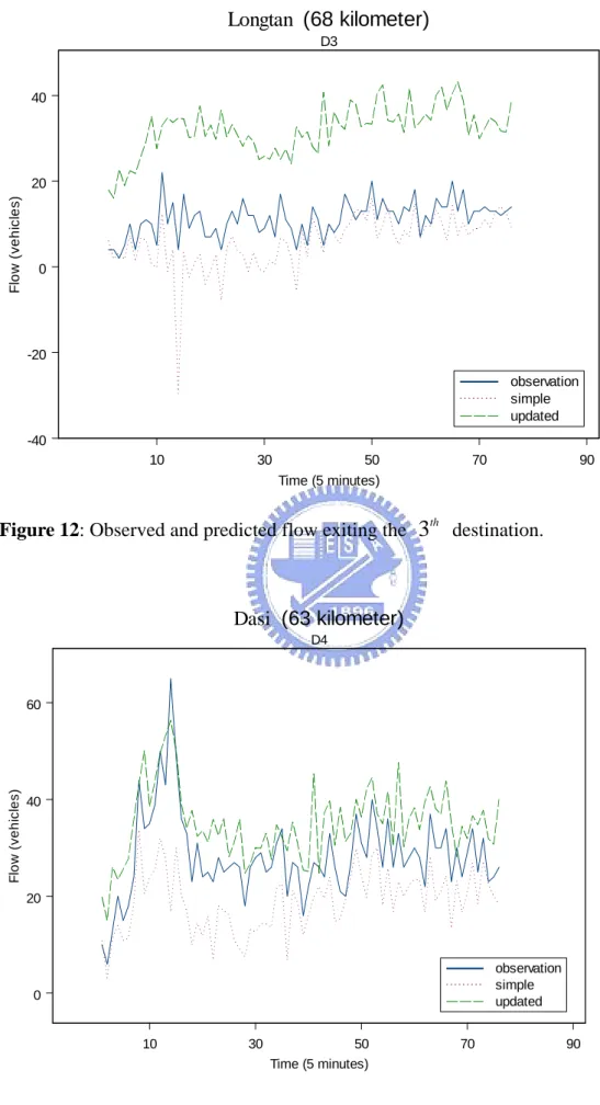
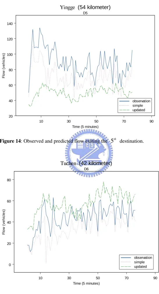
4.1 Data Collection 21 4.2 Data Analysis 23 4.3 Flow Prediction 24

5. Conclusion

37

6. References

38

1 Introduction

The origin-destination (O-D) flow plays an important role of most traffic operational analyses. The O-D flow has been used on the traffic assignment and the traffic flow simulation. Traditionally the O-D data collection is based mainly on field surveys, which not only costs a lot of budget, labor, and time, but also causes missing values easily when the traffic is heavy. Traffic engineers have been looking for statistical methods to estimate the O-D flow from less expensive data. Recent researchers estimate the O-D flow using Gaussian state-space model with an unknown transition matrix and Kalman filter but without considering the time factor. As the development of ITS (intelligent transportation system) changing with each passing day, the traditional traffic information becomes useless in the ATMS (advanced traffic management system). In order to achieve the aim of traffic control, the real time forecasts and estimates of the traffic condition in the future are desirable since the information can be used not only for ramp metering control but also for informing drivers the relevant information through the VMS (variable message sign) or HAR (highway advisory radio) to avoid the jammed traffic and save the travel time. Traditionally, researchers predict the O-D information ignoring the travel time which will produce erroneous results, especially when the travel time is long. In this thesis, we will investigate estimation of the O-D matrix with the travel time factor being taken into consideration in the dynamic system.

Here we briefly state that the state-space model consists of the state equation, representing the transition of the state variables, and the observation equation, describing the relationship between the state variables and the present and time lagged observations. An adaptive Monte Carlo technique known as the Gibbs sampler will be

used to estimate the unknown transition matrix and more importantly, the state variables in the state equation of the state space model. The classical state-space model was as follows:

1

1 +

+

=

t

+

t t

Fx

v

x

, called the state equation,

t t t

H

x

w

y

=

′

+

, called the observation equation,

where and are errors and if they process Gaussian distribution we called the model Gaussian state-space model. The Kalman filter algorithm is used to predict the stat variables since it gives the optimal predicted values when the model is Gaussian. To included the time factor, the model is modified as follows:

t

v

w

_t

: the state equation,

1

1 +

+

=

t

+

t t

Fx

v

x

: the observation equation with time lagged,

∑

= −

+

′

=

d i t i t i t

H

x

w

y

0

and we will investigate in more detail in the next sections.

In the traditional Kalman filter, matrices

F

and

H

are assumed to be known in advance. But in fact we can only find the matrix

H

from the network. And under the assumptions, which are outside the system,

F

can easily cause the model behave not well enough when the traffic flow is unstable. Here we propose using the Gibbs sampler to solve this problem. In our model, we initialize matrix

F

as an identity matrix and then use the Gibbs sampler to estimate

F

from the full conditional distributions and the observations. The general procedure to estimate the state variable (the O-D flows) is as follows: First, use the speed data collected by sensors on the freeway to calculate the travel time. Second, we use the calculated travel times to determine whether the vehicles arrive in the specific time interval or not and this will help us to find out the incidence matrix

H

exactly. Third,

conditional on the transition matrix

F

obtained in the previous stage, the state variables are filtered by the Kalman filter. Fourth, after the filter is finished, we use the Gibbs sampler to estimate the matrix

F

and then repeat these steps till the output converges.

2 Literature Review

Estimation of dynamic O-D matrices from traffic counts in a transportation network has received increasing attention over decades. Traditionally, the O-D flow matrices are considered only for a certain time period of interest, and thus are estimated with the average traffic count data of that period. A comprehensive review of research along this line can be found in Nugyen (1984) and Cascetta and Nugyen (1988). Such methods are static in nature, relying on the prior O-D information. Vardi (1996) considered the problem of estimating the traffic intensity between all “source-destination pairs” of nodes of a communication network from repeated measurements by maximum likelihood estimation. Tebaldi and West (1998) addressed the network count inference problem from a Bayesian aspect. In their framework of inference, the previous information on the O-D matrices are required, which is unrealistic. Their approach is also static and not suitable for predicting future O-D matrices. Since the number of relations between traffic counts and O-D pairs is usually far less than the O-D pairs, difficulties arise and some additional assumptions are needed.

To extend the O-D estimation methods in a dynamic system environment, researchers (e.g., Nihan and Davis {1989} and Cremer and Keller {1987}) proposed the use of time series traffic counts to formulate the relationships and applied to small networks by the methods of least squares and maximum likelihood. Okutani (1987) proposed using the Kalman filtering procedures for forecasting the O-D flows in a dynamic system, but gave no description with respect to the dynamic traffic assignment proportions on which the model was based. All the results mentioned above were obtained by a system ignoring the travel time and therefore of limited applicability. Recently in order to fit the requirement of the ATIS (advanced traveler

information system) and ATMS (advanced transportation management system) of ITS (intelligent transportation system), researchers paid lots of effect on estimation and predicting of travel time. Dailey (1999) used the state-space model to describe the relationship between measurements from single loop detectors, Chen and Chien (2001) predicted the travel time using probe vehicles data, Coifman (2002) estimated the travel time by data obtained from dual loop detectors, and Petty et al. (1998) treated the cumulative upstream and downstream arrival vehicles as a stochastic process and estimated the probability density function of the travel time.

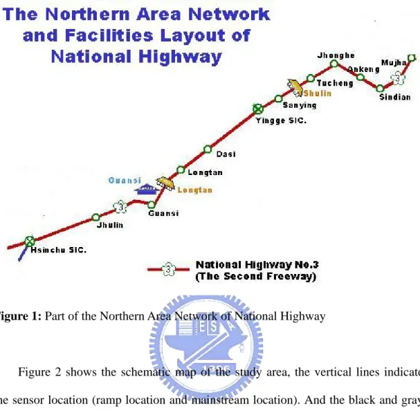
In this thesis, the state-space model will be combined with the concept of the travel time. Since it is relatively manageable in a highway system (the route choice issue is not involved), we will apply the proposed model to the data of National Highway No. 3. This thesis is organized as follows. The model specification and the algorithms used will be presented in Section 3. The empirical results are reported in Section 4. Conclusions and possible further enhancements are summarized in Section 5.

3 Model Specifications and Methodology

3.1 Problem Description and Notations

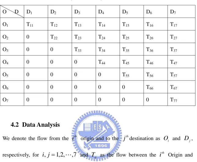
Suppose that a section of the highway system is divided into

N

segments so that each segment has only a pair of on- and off-ramps. Therefore, including the beginning and the ending segments, there are

N

+

1

nodes,

N

links and

N

origins and destinations, where the

i

th origin and the

(

i

−

1

)

th destination are the same ramp in the highway for

i

=

2

,

"

,

N

−

1

. The notations used in the model are listed as follows:

t i

O

, : the number of vehicles starting from the origin at time interval

th

i

t

for

N

i

=

1 "

,

,

; t j

D

_, : the number of vehicles exiting the

j

thdestination at time interval

t

for

N

j

=

1 "

,

,

;

t ij

T

_, : the number of vehicles entering the highway from origin to destination at time interval

th

i

j

th

t

for

1

≤

i

≤

j

≤

N

.

The ’s and ’s can be easily obtained from the detectors fitted in the

highway system, ’s are the unobserved variables of fundamental importance for the transportation planning and management purpose. The problem to be solved is to use the time series of link traffic flow { } and { } to estimate the time-varying

O-D flows { }. The state-space model is a natural alternative to specify the

relationship between the variables. The observations { } and { } will be

stacked up to form an observation vector, i.e.,

i

O

D

_j ij

T

t i

O

_,

D

_j,t t ij

T

_, t i

O

_,

D

_j,t

)

,

,

,

,

,

,

(

_{1, 2, , 1, 2, ,}

′

=

_{t t Nt t t Nt} t

O

O

O

D

D

D

y

"

"

,

)

,

,

,

,

,

,

,

,

,

(

_{11, 12, 1 , 22, 23, 2 , 1, 1, 1, , ,}

′

=

_{t t Nt t t Nt N− N− t N− Nt NNt} t

T

T

T

T

T

T

T

T

T

x

"

"

"

)

,

,

,

(

_{1, 2, ,}

′

=

x

_t

x

_t

"

x

_pt , where

p

=

N

(

N

+

1

)

2

.

Observe that , and that if the travel time could be ignored. Therefore, the basic model consists of a state equation indicating the transition of the state vector,

∑

=

=

N i j t ij t i

T

O

_{, ,}

∑

=

=

N j i t ij t j

T

D

_{, ,} , t t t

Fx

v

x

=

₋₁

+

and an observation equation indicating the relationship between

x

_t and

y

_t, , where

t t t

H

x

w

y

=

′

+

H

is a

p

×

q

incidence matrix with

q

=

2

N

.

3.2 The State-Space Model with Known Transition Matrix

3.2.1 State-Space Model

Let

y

_t denote a

q

×

1

vector of variables observed at time

t

, can be described in terms of an unobserved

t

y

1

×

p

vector called the state vector. The

state-space model is given by the following system of equations:

t

x

t t t

Fx

v

x

=

₋₁

+

,

t

=

1

,

2

,

"

,

n

(

1

)

t t t

H

x

w

y

=

′

+

,

t

=

1

,

2

,

"

,

n

.

( )

2

The development of the system over time is determined by s according to

trices

t

x

’

equation

( )

1

, but because

x

’s are not observed the analysis must be based on the observations

y

’s. The ma

t

dimensions

p

×

p

and

q

×

p

, respectively. Equation

( )

1

is known as the s

equation and equation

(2

observation equation. Th itial state variable

x

₀ is assumed to be

N

_p

(

₀

)

tate the 0

P

)

e in

,

µ

and independent of

v ,...,

₁

v

_n and

w ,...,

₁

w

_n, where

0

µ

and

P

₀ are assumed to be known. The

p

×

1

vectors

v

_t’s and the

×

1

tors

w

s are independent white noises su t

(

)

q

vec _t’ ch tha

E

v

_t

=

0

,

E

(

w

_t

)

Σ

(

v

_t

Cov

,

Cov

(

w

_t

)

=

Γ

, and

(

,

)

0

0

=

,

=

)

Cov

v

_t

w

_t

=

, for

t

=

1

,

2

,

"

,

n

, where

and are and atrices, respectively.

Typically w

v

are matrices

Σ

Γ

p

×

p

q

pos ariance m assume

~

(

0

,

Σ

)

. .

N

and

~

(

0

,

Γ

)

. . . q d i i t

N

w

,

v

_t’s and

w

_t’s

q

×

itive definite cov

e . p d i i t

independent, and the

Σ

and

Γ

a o ive defi e. Equation has the structure of the linea odel and equation represents a vector autoregressive model, where the Markovian nature accounts for many of the properties of the state-space model. And the assumptions enable updating of estimates via the Kalman filter easily.

re known and p sit nit

( )

2

r regression m

3.2.2 Kalman Filter

1 t

t

x

x

y

"

be the forecast of based on the info ion up to time

( )

1

Let

x

ˆ

_t+1|t

=

E

(

x

_t+1

|

y

₁

,

"

,

,

,

,

)

x

_t+1

rmat

t

and abbreviate as t

− t t

x

x

"

ecasts is r e foll | 1 1 | 1 | 1

he form

E

(

x

_t+1

|

y

_t

)

. The Kalman filter calculates these forecasts recursively, generating

ˆx

_1|0

,

₁ in succession.

The mean squared error (MSE) of the for epresented by th

| 1 | 2

,

,

ˆ

ˆ

t t

x

ˆ

+1| owing

p

×

p

matrix :

[(

x

_t+1

−

x

ˆ

)(

−

ˆ

)

′

]

E

P

_t+t

≡

_t+t

x

_t+

x

_t+t

( )

3

From

( )

1

we have

x

F

y

x

FE

y

Fx

E

y

| 1

|

t

)

(

t

|

t

)

(

t

|

t

)

ˆ

tt t t t

E

x

x

ˆ

1|

(

+

=

=

≡

.

Substitu ng it into equation , we have

, where

≡

+ ti

( )

3

P

_t+1|t

=

FP

_t|t

F

′

+

Σ

( )

4

]

)

)

|

(

))(

|

(

[(

|t

≡

t

−

t t t

−

t t

′

t

E

x

E

x

y

x

E

x

y

P

denotes the MSE of updating of

en becomes available. Next consider f

t t

y

t

x

wh orecasting the value of

y

_t. Let

)

|

(

1 1 − −

≡

t t

E

y

x

. From equation t

y

ˆ

_|

( )

2

, 1

)

|

|

(

₋ 1 | 1 1 |

(

)

ˆ

ˆ

tt₋

=

E

y

_t

x

_t

=

H

′

E

x

t

x

t₋

=

H

′

x

tt₋

y

.

From equation the MSE of this forecast is

( )

5

( )

3

=

′

−

−

_{− −} −

E

y

y

y

y

M

_{t|t 1}

≡

[(

_t

ˆ

_{t|t 1}

)(

_t

ˆ

_{t|t 1}

)

]

H

′

P

_t|t−1

H

+

Γ

.

After predicting the value of , we can update the current value of on the basis

pr ng tion: − − − −

−

′

×

−

−

×

( )

6

t

y

x

_t

of the observation of

y

_t to oduce

x

ˆ

_t|t

=

E

ˆ

(

x

_t

|

y

_t

)

. This can be evaluated using the formula for updati a linear projec

1 | 1 | 1 | | − − −

)

ˆ

(

]}

)

ˆ

)(

ˆ

[(

{

]}

)

ˆ

)(

ˆ

[(

{

ˆ

ˆ

1 | 1 1 | 1 |

′

−

−

+

=

tt t tt t tt t t

x

E

x

x

y

y

x

t t t t t t t t t

y

y

y

y

y

y

E

then we have 1 | 1 1 | 1 | 1 | − − − − −

( )

7

ˆ

_t|t

=

x

ˆ

_tt

+

P

_tt

HM

_tt

(

y

_t

−

H

′

x

ˆ

_tt

)

.

x

( )

8

From

P

_t|t

≡

E

(

x

_t

−

E

(

x

_t

))(

x

_t

−

E

(

x

_t

)

)

′

we have 1 | 1 1 | 1 | 1 | | − − − − −

−

′

=

_{tt tt tt tt} t t

P

P

HM

H

P

P

.

( )

9

Therefore, the recursion for predicting

x

_t+1 when

y

_t comes in can be expressed as follows:

)

ˆ

(

ˆ

ˆ

1 _{| 1} 1 | 1 | | | 1 − − − − +t

=

tt

+

tt tt t

−

′

tt t

F

x

FP

HM

y

H

x

x

)

ˆ

(

ˆ

_|

+

−

′

_|−1

≡

F

x

tt

K

t

y

t

H

x

tt ,

where is the Kalman gain matrix

p filter is summarized below.

tep 1 Initialize by giving the initial values

( )

10

t

K

.

The com lete procedure of the Kalman

S

x

ˆ

₀

=

E

(

x

₀

)

=

µ

₀

=

0

_p×1,

value of (

0 0

)

(

x

P

Cov

=

and let the predicted

x

₁

x

ˆ

1|0

=

µ

1|0) with no

observations be

F

µ

₀ , and therefore has MSE

P

_1|0 uation

(4

Predict the state v ble

x

_t with information up to time

−

1

from eq . Step 2 aria

)

t

1 1 | 1

)

|

(

x

t

y

t₋

≡

tt₋

=

F

E

µ

µ

t₋ ,

Σ

+

′

=

=

− _{− t|}1₋ −

P

FP

F

y

x

Cov

(

t

|

t 1

)

t|t 1 t 1 . Step 3 Predict − − − t

y

)

|

(

y

t

y

t 1

=

y

ˆ

t|t 1

=

H

′

t|t 1

E

µ

,

Γ

+

′

=

=

_{− −} −

M

H

P

H

y

y

Cov

(

t

|

t 1

)

t|t 1 t|t 1 . arameters − − −

Step 4 Update the p

)

ˆ

(

_{| 1} 1 1 |

−

1 | 1 | |

=

−

+

−

≡

_{tt tt tt} t

µ

µ

P

HM

tt

y

t

y

tt

µ

, 1 | 1 1 | 1 | 1 | | − − − − −

−

′

=

≡

_{tt tt tt tt tt} t

P

P

P

HM

H

P

P

,

1

+

= t

t

.

Step 7 Go to step 2.

3.3 Gibbs sampler

The Gibbs sampler is a statistical method for generating random variables from a join itional distributions without deriving the actual density. Giv

t distribution via cond

en an arbitrary starting values

(

,

2(0)

,

,

(0)

)

) 0 (

1

Z

Z

k

Z

"

, we start the sampling as follows: ( )

[

( ) ( ) ( )0

]

3 2 1 1 k , 0 0 1

,

,

,

|

~

Z

Z

Z

Z

Z

"

( )

[

( ) ( )0 ( )0

]

3 0 1 2 1 2

~

Z

|

Z

,

Z

,

,

Z

k

Z

"

,

#

( )

[

( ) ( ) ( )0

]

1 0 2 0 1 1

,

,

,

|

~

k K₋ k

Z

Z

Z

z

Z

"

.

Then we have a new set of values

(

Z

₁( )1

,

Z

₂( )1

,

"

,

Z

k( )1

)

to continue the iteration.

After m such iterations we have

(

Z

1( )m

,

Z

2( )m

,

"

,

Z

_k( )m

)

. The paper of Geman and

Geman showed that the following results hold under mild conditions.

1.

(

1984

)

( ) ( ) ( )

(

m m m

)

(

)

( )m d

∞

→

m

k k

Z

Z

Z

Z

Z

Z

₁

,

₂

,

"

,

→

₁

,

₂

,

"

,

and so that for each

Z

_i

→

Z

as

For any Borel measurable function

i

, _i . 2.

T

of

(

Z

₁

,

Z

₂

,

"

,

Z

_k

)

wh seo expectation exists, ( ) ( ) ( )

(

)

(

(

k

)

)

s a m

1

.. j j k j j m

_m

T

Z

,

Z

,

,

Z

E

T

Z

,

Z

,

,

Z

lim

_{1 2} 1 2 1

"

→

"

∑

= ∞ → .

3.4 State-Space Model with unknown Transition matrix

From state-space model, equation

3.4.1 Estimation of F by Gibbs Sampler

( )

1

can be written as

,

"

t

N

v

Fx

x

v

_t

=

_t

−

_t−1

,

_t

~

_p

(

0

,

Σ

)

=

1

,

2

,

n

.

The joint distribution of

V

=

(

v

₁

,

v

₂

,

"

,

v

_n

)

′

is

)

2

1

exp(

|

|

)

,

|

(

1 1 2

∑

= − −

₋

′

_Σ

Σ

∝

Σ

n i i i n

v

v

F

V

p

. Denote

( )

11

)

(

F

S

to be the

p

×

p

symmetric matrix

S

( )

F

=

{

S

_ij

(

F

_i

,

F

_j

)

}

with

1 1

−

=

"

−

=

⋅

=

∑

v

v

∑

x

F

x

x

F

x

i

j

p

F

F

S

n u n u u j uj u i ui uj ui j i ij

(

,

)

(

)(

)

,

,

1

,

2

,

,

1 1 = = − − ,

where denote the row of

( )

12

i

F

th

i

F

.

Then the exponent in

( )

11

can be expressed as

)

)

(

2

1

exp(

− trS

Σ

−1

F

From the transition equation of

( )

13

( )

1

we have

x

_t

′

=

x

_t

′

₋₁

F

′

+

v

_t

′

,

t

=

1

,

2

,

"

,

n

Let

_⎢

⎢

_⎥

⎥

⎥⎦

⎤

⎢⎣

⎡

′

′

=

⎥

⎥

⎢

⎢

=

′

⎥

⎥

⎢

⎢

=

′

_n− n

X

X

#

#

'

#

1

,

, t e

⎥⎦

⎤

⎢⎣

⎡

′

′

⎥⎦

⎤

⎢⎣

⎡

′

′

− n n n

v

v

V

x

x

x

x

₁ 1 0 1

,

hen the transition equation has th

of a linear model: form

V

F

X

X

_n

′

=

_n

′

₋₁

′

+

′

X

F

F

S

( )

14

and equation

( )

12

can be expressed as

)

(

)

X

X

F

F

X

(

)

,

(

_{i j n(i) n1 i n(j) n 1 j} ij

=

′

−

′

−

′

′

′

−

′

−

′

,

( )

15

where

X ′

_n(i) denotes the

i

th column of

X ′

_n.

Let denote the least square estim

n

16

be 1 ) (i n i n n j i ij

F

F

=

X

′

−

X

′

−

F

′

− Consequently, , wh 1 1

F

X

n j

X

n

F

n i n ij −

′

′

−

−

′

ters ) ( 1 1 1 1

)

(

ˆ

i n n n n i

X

X

X

X

F

′

=

₋

′

₋ − ₋

′

ator of

F

_i

′

, so that

equatio

(

)

can further rewritten as

)

ˆ

(

)

ˆ

(

)

ˆ

(

)

X

_n(j)

X

_{n 1}

F

_j

F

_i

F

_i

X

_n1

X

F

_j

F

_j

S

′

′

′

−

′

₋

′

+

′

−

′

′

₋

′

−

′

ˆ

(

)

,

(

₁

( )

16

)

ˆ

(

)

ˆ

(

)

(

F

A

F

F

X

1

X

1

F

F

S

=

+

′

−

′

′

n−

′

n−

′

−

′

( )

17

ere

A

=

{

a

_ij

}

is a

p

×

p

matrix with

( )

ˆ

)

(

( )

ˆ

)

(

X

X

a

=

−

For the prior distribution of the parame

(

F

,

Σ

)

, we shall first assume that

F

and

Σ

are approximately independent so that

)

(

)

(

)

,

(

F

Σ

≈

p

F

⋅

p

Σ

p

ant

const

F

p

(

)

∝

and it is appropriate to take F as locally uniform, i.e. . Then the rior distribution of joint poste

(

F

,

Σ

)

is

)]

(

2

exp[

|

|

)

,

|

,

(

1 ( 1) 2

_tr

X

X

F

p

n n n p + + − −

∝

Σ

−

Σ

( )

18

and by changing of variable w

1

1 1

F

S

−

Σ

, e have

)]

(

2

1

exp[

|

|

)

,

|

,

(F

p

1 ₁ 1 2( 1) 1

( )

1

F

S

tr

X

X

_{n n−} − n−p− − −

_∝

_Σ

₋

_Σ

Σ

,

marginal posterior distribution of

19

F

is the Wishart distribution. Then the has the

lowing form fol 2

|

)

(

|

)

,

|

(

F

X

X

₁

S

F

p

_{n n−}

∝

′

,

( )

20

from equation

( )

n − we have

15

2

|

)

ˆ

(

)

ˆ

1 1 n

F

F

X

X

F

′

′

_{n− n}

′

₋

′

−

′

−

−

( )

(

|

)

,

|

(

F

X

X

₁

A

F

p

_{n n−}

∝

+

′

21

Theorem 1. [Johnson and Kotz (1972)]

T

be the random

p

×

q

matrix,

T

U

1

X

)

(

2 1 ₋

′

=

, Let

X

where

U

~

W

_p

(

P

,

m

−

q

)

,

m

>

p

+

q

−

1

, independently of , the distribution of the tran ose of each row of sp

X

,

x

_i

′

, is denoted by

x

_i

′

~

N

_q

(

0

,

Q

)

;

P

and

itive definite. The jo d ty functio

Q

are pos int ensi n of

T

is

m q m

P

T

Q

P

Q

q

p

m

k

T

p

2 1 2 1

|

|

|

|

)]

,

,

(

[

)

(

=

−1

×

(

+

′

These results were obtained by Dickey (1967)

p

T

2 1

|

|

− ) − istribution of

F

According to the above theorem, the marginal d with corresponding eters, and ,

param

p

=

q

m

=

n

n

> p

2

−

1

, can be written as

2 2 2

|

|

|

(

ˆ

)

|

|

|

)

(

F

A

( )

X

₁

X

₁

A

F

F

X

₁

X

p

′

∝

n p _{n− n}

′

₋ p

+

′

−

′

′

_{n− n}

′

Sampling sch 1 1 1 n

F

− − −

eme: generate

x

_t and

F

from ribution. tep 1

the conditional dist

)

,

(

~

,

,

|

_t−1

Σ

_{p t−1}

Σ

t

F

x

N

Fx

x

S Step 2

F

′

|

X

_n

,

X

_n−1

,

Σ

~

p

(

F

′

|

X

_n

,

X

_n−1

)

Generate

W

~

W

_p

(

n

−

p

,

X

_n−1

X

_n

′

₋₁

)

1 2 Generate

Z

=

(

z

₁

,

z

₂

,

"

,

z

_p

)

′

and 3

)

,

0

(

~

N

A

z

_{i p} Let

F

[(

W

2

)

]

1

Z

1 −

′

=

′

3.4.2 G u

a ssian state s ace without considering travel time

p

In Section 3.2.2 we use Kalman filter to update the parameter vector after observing the new observation

y

_t. In a traditional state-space model, the transition

matrix

F

is known before we start to filter the stat vector by Kalman filter. But in reality

F

is usually unknown, one way to solve this problem is to combine Gibbs sampler with Kalman filter. The complete algorithm is summarized as follows:

Algorithm 1 (Gaussian state space model without considering travel time)

Step 1 (Initialization)

1. given the initial value of

F

(0)

=

I

_p×p

2. Given

Σ

and

Γ

3. Given

µ

₀

, P

₀ to generate

x

₀(g) from

N

_p

(

µ

₀

,

P

₀

)

4.

g

=

0

Step e

x

tg ) ( ) Generate from 2 ( eneratG

,

t

=

0

,

1

,

2

,

"

,

n

) ( g t

x

N

_p

(

µ

_t

,

P

_t

)

1. ) ( 1 | g t t

x

₋ from

|

,

~

(

(1)

,

)

) ( ) ( ) ( 1 −

Σ

− g t g p g g t t

x

F

N

F

x

x

an f filter (here we update 2. Generate

3. Use the Kalm ilter to

x

_t( g)

µ

_t and ) ilter the part of predicting of we use

− t t t 4. t

P

3.1 In Step 3 of the Kalman f

y

_t

1 |

ˆ

ˆ

= x

H

′

y

to predict

y

_t Repeat 2,3 for

t

=

2

,

3

,

"

,

n

) ( g

F ′

Step 3 (Generate ) 1. Calculate

X

_n(₋g₁ (1) ) g n

X

′

₋ − − ( 1 ) (

)

(

n ig g n g n g n g i

=

X

′

X

′

−

X

′

− − − 2. Calculate

=

{

},

(

ˆ

)

(

(1)

ˆ

( )

)

) ( ) ( ) ( ) ( 1 ) ( ) ( ) ( ) ( ) ( g j g n g j n g i g n g i n g ij g ij g

F

X

X

F

X

X

a

a

A

=

′

−

′

′

′

′

−

′

′

where

F ′

ˆ

)

X

(()) ) ( 1 1 ) ( 1 3. Generate

~

(

( )

,

)

1 ) ( 1

X

n

p

X

W

w

g n g n p −

′

−

−

4. te

(

₁

,

₂

,

,

)

,

~

_p (g) iid k p

z

N

A

z

z

z

Z

=

′

′

"

′

′

Genera

(

0

,

)

Z

w

F

(g) 1

)

)

((

2 1 ₋

′

=

′

5. Generate 6.

g

= g

+

1

, if

g

<

m

go to step2 Step 4 (Prediction)

Then we have

{

X

(1)

,

"

,

X

(m)

}

. At last, we will have the estimator

∑

=

m

X

X

ˆ

1

(

∑

− =

′

=

′

m k m g g

F

k

F

ˆ

1

( )

)

(

m

>

k

− =m k g g

k

) and

After having , the predict of the state vector can be obtained according to

with

Fˆ

( )

10

F

replaced by .

3.4.3 Gaussian state space model with considering travel time

In modeling the interrelation between O-D flow matrix and link flow in a freeway

time from one place to the destination. In

this O-D

estim

Fˆ

network, it is unrealistic to ignore the travel

thesis, we propose a more adequate state-space model for dynamic ation by taking into account the travel time required by each trip. The incident matrix in the observation equation

H ′

is a matrix with elements ones and zeros

t

contribute to affect the observation at the same

depending on whether or not the elements of

x

the path flow will or will not

ti

y

t

, i.e. the travel time is ignored.

By considering the travel time required form on place to another,

y

_ti, the link flow obtained at time interval

t

is accum ated by the path flows possibly occurred from several time intervals before. Therefore, the interrelationship between

y

_t and

x

_tcan be formulated by the following model:

t t t

Fx

v

x

=

₋₁

+

,

t

n

d

w

x

H

y

t i t d i t

=

∑

′

−

+

,

<

,

n

i

,

,

2

,

1

0

"

=

= .

here

x

_t

=

(

x

_t1

,

x

_t2

"

x

_tp

′

is the state vector at time

( )

22

w

,

,

)

t

,

t

=

1

,

2

,

"

,

n

and

enotes the number of vehicles traveled at time

tj

x

p

j

=

1

,

2

,

"

,

t

of O-D pair

j

,

,

erved vector at time i

d

the obs nterval

t

,

=

(

₁

,

₂

,

"

,

y

_tq

)′

, and e

t t t

y

y

y

_ti is the

counts of vehicles entering or exiting the

i

th nod ,

i

1

,

2

,

"

,

q

y

=

.

)

,

,

1

,

0

(

i

d

H

′

=

is the

q

×

p

O-D pair zero-one as its

elements, and

H

H

d

′

=

′

∑

in the equation

i

"

incident matrices with

=0

i

i

( )

2

of the standard state-space model.

The number is

MSE of the predictor

E

x

_t+1

y

_t ,

1 |

1

d

the max number of time periods needed for a path flow contributing the corresponding link flow.

We will use the same notation as in the previous derivation

x

ˆ

_t+1|_t representing

the forecast of

x

_t+1 based on

y

_t. The imum

)

|

(

ˆ

_{t 1t|}

x

₊

=

]

)

ˆ

)(

ˆ

[(

−

1| 1

−

1|

′

=

E

x

x

x

x

P

can be expressed as

′

+

Σ

.

The next stage of predicting the value of

y

:

y

ˆ

E

y

x

+ + + + +t t t t t t t t 2 1 1 |t t t t t m t − −

x

−

x

−

=

+

FP

F

P

t 1|t t|t t

=

(

|

,

,

"

,

)

from equation we have i i t t

x

y

E

₋ =0

)

|

(

d i i t i t t t t t i t i i t t t t

H

x

H

H

x

2 1 | 1 1 1 | 0 1 0 1 1 |

ˆ

µ

where the d

x

H

∑

′

=

and then

( )

18

_{t i}

∑

∑

= − − − − − − = − −

=

=

′

=

′

+

′

+

′

d

x

x

E

H

x

y

E

y

ˆ

(

|

)

(

|

)

( )

23

)

|

(

1 1 1 | 1− − − −t

=

t t t

E

x

x

µ

. The MSE of the predictor

y

ˆ

_t|t−1 is as follows:

]

)

(

)

ˆ

(

)][

(

)

ˆ

(

[

0 | 1 1 1 1| 1 0 | 1 1 1 1| 1 1 |t−

=

′

t

−

tt−

+

′

t−

−

t−t−

′

t

−

tt−

+

′

t−

−

t−t−

′

t

H

x

x

H

x

H

x

x

H

x

M

µ

µ

′

′

′

+

+

′

+

′

+

Γ

′

=

H

0

P

t|t₋1

H

0

H

1

P

t₋1|t₋1

(

H

0

F

)

(

H

0

F

)

P

t₋1|t₋1

H

1

H

1

P

t₋1|t₋1

H

1

(24

)

1 1 | 1 | 1 | | − − − −

−

×

′

−

−

×

{

[(

ˆ

)(

ˆ

)

]}

(

ˆ

)

]}

)

ˆ

)(

ˆ

[(

{

ˆ

ˆ

1 | 1 | 1 |− − −

′

−

−

+

=

tt t tt t tt t t

y

y

y

y

y

y

E

y

y

x

x

E

x

x

then we have t t t t t t t t t

( )

25

x

ˆ

_t|t

=

x

ˆ

_t|t−1

+

(

P

_t|t−1

H

₀

+

FP

_t−1

H

₁

)

M

_t−_|t1₋₁

(

y

_t

−

y

ˆ

_t|t−1

)

( )

26

)

)

(

))(

(

(

|t

≡

t

−

t t

−

t

′

t

P

E

x

E

x

x

E

x

we have and from

P

_t|t

=

P

_t|t−1

−

(

P

_t|t−1

H

₀

+

FP

_t−1

H

₁

)

M

_t−_|t1₋₁

(

P

_t|t−1

H

₀

+

F

_{t−1 1}

)′

modify the original Kalman filter as

lues

H

P

( )

27

so we can bellow:

Step 1 Initialize the algorithm by giving the initial va

x

ˆ

₀

=

E

(

x

₀

)

=

µ

₀,

0 0

)

(

x

P

Var

=

and let the predict value of

x

₁ (

x

ˆ

1|0

=

µ

1|0) with no

observations be

F

µ

₀ , and therefore has MSE

P

1

=

0 | 1 .

and start with

t

estimating the ne age:

Step 2 xt st

F

t t

y

x

E

(

|

−1

)

=

µ

t|t−1

=

µ

t

Σ

+

′

=

=

₋ −

P

FP

y

x

Var

(

t

|

t 1

)

t|t 1 t|t

F

Step 3 prediction of (equation ) − −

=

tt t t (equation t

y

∑

= − − − − −

=

=

′

+

′

+

′

d i i t i t t t t t t t

y

y

H

H

H

x

y

E

2 1 1 1 | 0 1 | 1

)

ˆ

|

(

µ

µ

( )

23

|

(

y

y

M

Var

1

)

| 1

( )

24

)

′

+

′

+

′

′

′

+

′

=

H

0

P

t|t₋1

H

0

H

1

P

t₋1|t₋1

(

H

0

F

)

(

H

0

F

)

P

t₋1|t₋1

H

1 1 t₋1|t₋1 1 eters

Γ

+

H

P

H

Step 4 update the param

)

ˆ

(

)

(

| 1 1 1 | 1 1 0 1 | 1 | | − − − − − −

+

+

−

=

=

t

µ

tt

µ

tt

P

tt

H

FP

t

H

M

tt

y

t

y

tt

µ

(equation

( )

26

)

(

| 1 0 1 | |

)

(

| 1 0 1 1

)

1 1 | 1 1

+

′

+

−

₋ −

P

H

FP

P

P

tt

=

tt tt − − − − −

H

M

tt

P

tt

H

FP

t

H

t (equation

( )

27

)

1

+

= t

t

Step 5 if

t

=

n

stop ep 6 go to step 2 1 as:

l with travel time)

ep 1 (Initialization) St

And we can update the Algorithm

Algorithm 2 (Gaussian state space mode

St

1. give the initial value of

F

(0)

=

I

_p×p

2. Given

Σ

and

Γ

3. Given

µ

₀

, P

₀ to genera

(

,

,

,

0( )

)

) ( 1 0 ) ( 0 ) ( 0 g d g g g

x

x

x

X

=

₋

"

₋

te the prior state-matrix ,

0 0

P

p i where ( )

~

(

N

g

)

,

x

µ

for

i

=

0

,

−

1

,

"

,

−

d

4.

g

=

0

n

,

) Step 2 (Generate ( )

,

=

0

,

1

,

2

,

_"

Generate

t

x

g t

)

,

(

~

) ( t t p g t

N

P

x

µ

1. ) ( 1 | g t t

x

₋ from

|

,

~

(

( )

,

)

1 ) ( ) ( ) ( 1 −

Σ

− g t g p g g t t

F

N

F

x

2. Generate

x

x

an filter to filter

an filter the part of predicting of we use

d i g i t i t t t t

H

2 ) ( 1 1 1 |

0 to predict and change the

0 t t d t t − − − ilter 4. Repeat 2,3 for ) ( g t

x

3. Use the Kalm

The updated Kalm

y

_t

∑

′

+

′

+

′

=

g g

x

H

x

H

y

( ) ( )

ˆ

µ

= − − −

y

t matrix (g)

(

(g)

,

(g)

,

,

(g)

)

x

x

x

X

=

₁

"

to continue the f .

n

t

=

2

,

3

,

"

,

) ( g

F ′

) Step 3 (Generate