使用最少量緩衝器於延遲容忍系統中達成效能最佳化

國立交通大學

電子工程學系 電子研究所

碩 士 論 文

使用最少量緩衝器於延遲容忍系統中達成

效能最佳化

Throughput Optimization for Latency Insensitive

System with Minimal Buffer Size

研 究 生：何亞謙

指導教授：黃俊達 博士

使用最少量緩衝器於延遲容忍系統中達成

效能最佳化

Throughput Optimization for Latency Insensitive

System with Minimal Buffer Size

研 究 生：何亞謙

Student:

Ya-Chien

Ho

指導教授：黃俊達 博士

Advisor:

Dr.

Juinn-Dar

Huang

國立交通大學

電子工程學系 電子研究所

碩士論文

A Thesis

Submitted to Department of Electronics Engineering & Institute of Electronics College of Electrical & Computer Engineering

National Chiao Tung University in partial Fulfillment of the Requirements

for the Degree of Master

in

Electronics Engineering & Institute of Electronics July 2009

Hsinchu, Taiwan, Republic of China

使用最少量緩衝器於延遲容忍系統中達成

效能最佳化

研究生：何亞謙 指導教授：黃俊達 博士

國立交通大學

電子工程學系 電子研究所

摘 要

當製程進入深次微米尺寸，全局接線成為現今的系統單晶片設計

中最關鍵性的難題之一。延遲容忍系統(LIS)被提出來用於解決易變

的接線延遲且不需要改變原有的矽智財設計，延遲容忍系統避免掉了

在產品發展過程中會浪費大量時間的延遲調整，所以延遲容忍系統是

個很好的方法去加速產品設計過程。但是在不同接線上有不平衡的延

遲以及後端的停止要求都會讓延遲容忍系統的效能有所衰退。我們提

出了一個整數線性規劃公式去改善效能至最佳值並且使用最少量的

緩衝器，我們也發展了我們的圖形表示法—量化圖。並用依據量化圖

的特性，我們發展了一套降階流程去減小圖形大小但依舊維持正確

性。我們也考慮了實際上晶片上會有不同的頻寬。實驗結果顯示我們

的方法可以大幅降低圖形大小並且省下至少 20%的緩衝器。

Throughput Optimization for Latency Insensitive

System with Minimal Buffer Size

Student: Ya-Chien Ho Advisor: Dr. Juinn-Dar Huang

Department of Electronics Engineering &

Institute of Electronics

National Chiao Tung University

ABSTRACT

As manufacturing process proceeds to deep submicron (DSM) technology, global interconnect delay becomes one of the most critical obstacles in system-on-chip (SoC) design nowadays. Latency insensitive system (LIS) is a method proposed to solve variant interconnect delay without modifying pre-designed IP cores. In other words, LIS avoids modified delay iterations in product developed period. LIS offers a solution for time-to-market. However, the imbalance delay and back-pressure in LISs cause performance degradation. We propose an ILP formulation to improve performance to optimal value while maintaining minimal buffer size. We also propose a graph representation called quantitative graph (QG). Then we develop the reduction procedure on QG to decrease graph size while maintaining correctness of performance. We also consider practical situation which chip have different channel bit width on it. From the experimental results, our method reduces graph size greatly and our method saves more than 20% of buffer size than pervious works.

Acknowledgment

從進入研究所到這份論文的完成，我得到非常多人的幫忙以及關懷。我在此 對這些曾經幫助過我的人表達我的感謝之意，如果沒有你們的援手，也許這份論 文就無法完成。 首先我要感謝我的家人們。我的父母，辛苦的工作並養育我，給我一個衣食 無缺的環境，讓我能專注在自己的研究工作上。在研究的過程中也全力的支持 我，讓我無後顧之憂的完成我的研究，這篇論文能夠完成，我的父母佔了很大一 部份的功勞，我在此表達我對他們的感謝。 再來我要感謝我的指導教授─黃俊達教授。他提供了良好的研究環境並且鼓 勵我們多吸收新的知識。如果沒有阿達老師的教導、解惑、以及每個星期不間斷 的討論，我的研究勢必是沒有辦法順利完成的。所以在此再次感謝我的指導教授。 另外要感謝的是實驗室所有的學長姐及同學，尤其是耿維學長從我進研究所 後就不斷幫助我了解、修正研究的內容，小形、莎莉，克莉絲塔兒學姐在課業及 研究上給我的建議跟幫助，家宏、步青、篤雄、建德、瀚蔚學長在我遇到困難時 的提攜跟解決問題，還有同屆的同學們一路上的互相扶持，彥廷、智宏、毓翔、 于翔、婉玲，謝謝你們陪我一起度過兩年愉快的研究所生活。 最後，一份論文的產生實在需要很多很多的助力，不管是直接的，或是間接 的，我受到的幫助實在太多，無法一一列舉感謝，所以最後還是要對這一路上曾 幫助過我的人表示最真誠的感謝。

Contents

Abstract(Chinese) ... i Abstract(English) ... ii Acknowledgment ...iii Contents ... iv List of Figures ... vi

List of Tables ...viii

Chapter 1 Introduction ... 1

1.1 Motivation... 4

1.2 Contribution ... 5

1.3 Thesis Organization ... 6

Chapter 2 Preliminaries... 7

2.1 Latency Insensitive System (LIS)... 7

2.2 Throughput Optimization for Latency Insensitive System... 12

2.2.1 Relay Station Insertion... 13

2.2.2 Queue Sizing... 14

2.3 Related Works... 15

Chapter 3 Throughput Optimization for LIS with Minimal Buffer Size ... 18

3.1 Marked Graph and Quantitative Graph (QG) ... 18

3.2 Quantitative Graph Reduction ... 22

3.2.1 Path Condensation... 23

3.2.2 Edge Unification ... 24

3.3 Problem Formulation of Our Approach... 28

Chapter 4 Experimental Results... 32

4.1 Environment Setup and Benchmarks... 32

4.2 Weight and Channel Latency Assignment... 33

4.3 Results... 33

4.3.1 Experiment Ⅰ... 34

4.3.2 Experiment Ⅱ... 35

4.3.3 Experiment Ⅲ... 37

4.4 Discussion... 38

Chapter 5 Future Works and Conclusions ... 40

List of Figures

1-1 Un-scaling global interconnect as device size shrinking down... 1

1-2 Delay for global interconnects, local interconnects and gate (cited from [3]) ... 2

1-3 An example of the pipeline element insertion ... 4

2-1 Shell encapsulation and RS insertion in an LIS ... 8

2-2 Block diagram of an encapsulated IP core ... 9

2-3 Progressive trace of a simple LIS ... 9

2-4 Output data sequence at core C in Figure 2-3 ... 10

2-5 Simple LIS example with inserted relay station and back-pressure... 11

2-6 Output data sequence of core C in Figure 2-5 ... 12

2-7 Optimize throughput by inserting relay station ... 13

2-8 Counter example of relay station insertion... 14

2-9 Optimize throughput by queue sizing... 15

3-1 Modeling relay station and shell with marked graph representation... 18

3-2 Transformation from original LIS graph to marked graph representation ... 19

3-3 Queue sizing problem reflects to marked graph representation ... 20

3-4 Transformation from a marked graph to a quantitative graph... 21

3-5 Two graphs are equivalent in throughput calculation ... 23

3-6 Operation of edge unification ... 25

3-7 Total reduction procedure of an LIS example ... 26

3-8 An example of recovered procedure step 1 ... 27

3-9 An example of recovered procedure step 2 ... 27

3-10 Queues are added to different positions ... 29

4-1 The flowchart of our experiments ... 32

List of Tables

4-1 Number of cycles degradation after the reduction procedure performed... 34

4-2 Experimental results when channel latency locates on [1, 3]... 35

4-3 Experimental results when channel latency locates on [1, 5]... 36

Chapter 1

Introduction

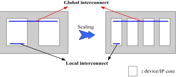
As the manufacturing process proceeds to deep submicron (DSM) technology, device size and interconnect width continuously scale down. This evolutionary scaling makes individual device speed become significantly faster; however, it also makes the delay of interconnect become worse. As a result, interconnect delay problem has become one of the most critical obstacles for designs nowadays. Interconnect delay problem suffers from increased resistance due to a decrease in conductor cross-sectional area and also suffers from increased capacitance when metal height is not reduced with conductor spacing [1]. Another reason that interconnect delay problem turns into the boundary of designs is the failure of global interconnect scaling. The length of global interconnects can not shrink down as devices and local interconnects. As Figure 1-1 [2] shows, global interconnects must pass through multiple IPs in order to connect them together. From the figure, global interconnects keep unchanged while local interconnects and devices shrink down with process scaling.

Due to the un-scalable characteristic of global interconnects, the relative delay difference between global interconnects and local interconnects broadens. Figure 1-2, which is cited from [3], shows the trend for relative delay gap in different process generation. The global interconnect delay is about twenty times slower than gate delay and is about sixteen times slower than local interconnects delay in 65nm process. The circumstance gets worse in 32nm, where global interconnects delay is one hundred and twenty times slower than local interconnects delay.

Figure 1-2. Delay for global interconnects, local interconnects and gate. (cited from [3])

Figure 1-2 implies that length of global interconnects has grown rapidly compared to local interconnects so a signal can not arrive from one side to the other side within a clock cycle. Hence, it is unavoidable that the data transfers between IPs require multiple clock cycles to deliver. Such multi-cycle communication can seriously degrade the performance improvement originally obtained from advanced fabrication technology. The acceleration of individual devices and the multi-cycle

communication bottleneck force designers to shift design paradigm from computation-bound to communication-bound.

There has developed some technologies to ease the communication burden caused from global interconnects delay. In physical design level, wire sizing, buffer insertion…and so on, help to relax the delay constraints. In system design level, many research works try to not only conquer the communication bottleneck but also maintain the functional behavior unchanged.

One approach is to utilize asynchronous handshake protocols for global inter-core communication. This is called globally-asynchronous locally-synchronous (GALS) systems [4]–[6]. Another one is network-on-chip (NoC) platform in [7] and [8], which constructs an on-chip interconnection network for global signals transmission. The data transmission in NoC passes through every module’s router with helping of those on-chip network interfaces. [9] and [10] propose a regular distributed register (RDR) microarchitecture which is composed of array of islands. Communication inside an island can be finished in a single clock cycle. For multi-cycle communication between islands, layout-driven architectural synthesis algorithms have been developed.

There is another method called Latency Insensitive System (LIS) reported in [11] and [12] which is receiving many attentions recently. The LIS approach does not alter original system architecture but it wraps every IP with a special interface and adds small pipeline elements to systems. By using those additional elements and interfaces, LISs cope with variant interconnect delay without changing any IP in the system. Inserting pipeline elements into global interconnects, like LIS design paradigm, is the

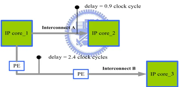
design mainstream for synchronous system nowadays [13]. Timing constraints are relaxed after inserting pipeline elements into long interconnects so that loose timing constraints can lead to operating frequency acceleration. For example, the interconnects shown in Figure 1-3, the input/output timing constraints of all interconnects are needed to be smaller than 1 clock cycle. For instance, the delay of interconnect A is 0.9 clock cycle such that it needs no pipelining. On the other size the delay of interconnect B is 2.4 clock cycles such that it needs two pipeline elements inserted into interconnect B. Because of it, the input/output timing constraints of interconnect B are feasible.

Figure 1-3. An example of the pipeline element insertion.

1.1 Motivation

As the complexity of system-on-chip (SoC) keeps growing, it is impossible to redesign each IP for a new system. According to that reason, IP reuse becomes the most promising way in present SoC design. However, length of interconnects is

unpredictable at early design stage. It makes engineers hard to determine the exact time when IPs should receive and send data. Interconnect length information remains unknown until the floorplanning is actually performed. In other words, how many clock cycles are needed for data communication is dependent on the result of floorplanning. If the timing after floorplanning do not meet the requirement, it may jeopardize system performance, or even worse, ruin the overall system behavior. Therefore, engineers need to adjust floorplanning appropriately or redesign IPs to accommodate multi-cycle communication. Time wasted on adjusting floorplanning or redesigning IPs is significantly long that may be a terrible damage to project schedule. Hence, it is urgent that we need an efficient method to solve multi-cycle communication and IP reuse dilemma. Latency Insensitive System is a correct-by-construction methodology and seems to be a promising solution that can solve both problems at the same time. As a result, we consider LIS as the greatest time-to-market method in the incoming era of high speed synchronous design and we adopt LIS to achieve optimal performance while maintaining minimal area cost.

1.2 Contribution

In this thesis, we propose an ILP formulation to solve LISs for optimal throughput solution with minimal area. We follow the marked graph representation to model LIS and we transform original marked graph to quantitative graph for latter reduction operations. When we use marked graph to during ILP formulation, number of cycles in the graph are the limitation to the ILP formulation. It needs a lot of time to get the optimal solution for larger practical cases. This may be the obstacle of project schedule. We propose a procedure which contains two operations to deal with this obstacle. Path condensation and edge unification are used to reduce graph size so

that we can handle bigger design cases. All benchmarks can be solved within 20 minutes in our experiments after the reduction procedure is performed. Then, our proposed ILP formulation finds the minimal buffer size to achieve optimal performance. To reflect real situation in the SoC system, we take bit width issue into consideration. In the end, we obtain optimal solution on buffer size while maintaining optimal performance and have faster computation speed to get that optimal solution.

According to the experimental results, it is concluded that the reduction procedure decreases graph size greatly. Furthermore, our approach performs better when interconnect delay becomes worse. Finally, when bit width issue is also considered, the difference of results between our approach and previous works become larger.

1.3 Thesis Organization

This thesis is organized as follows. In Chapter 2 we give the preliminaries of our work. It includes the introduction of latency insensitive system, how to fix system performance degradation of LIS caused by multi-cycle communication, and some related works. The proposed strategy for performance optimization with minimal buffer size is given in Chapter 3. The experimental results and related analyses are provided in Chapter 4. Chapter 5 concludes this thesis and lists probable future works.

Chapter 2

Preliminaries

2.1 Latency Insensitive System (LIS)

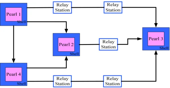
The concept to design a system which is insensitive to arbitrary variation in interconnect delay was first presented in [14]. The proposed approach Latency insensitive design (LID) is a design methodology for SoC that enables automatic adjustment to original system in order to make new system get with variant delay. LID encapsulates each IP core (the pearl) with an automatically-synthesized interface (the shell) and inserts repeaters to pipeline long interconnects. Those repeaters are called relay stations (RS) in LIS. By using LID, one can derive an LIS from original synchronous system. IP cores may be synchronous sequential logic blocks of any complexity as long as they satisfy the stallability, i.e., their operation can be temporarily stalled [12]. Relay stations are clocked buffers with two-fold storage capacity used to pipeline every long interconnect in order to let them meet the target clock period. After doing those movements, an LIS is latency-equivalent to original synchronous system [12]. It means that when we ignore stalling (void) events in timestamps, the rest informative (valid) events on each channel of an LIS are exactly the same with the informative events on each channel of the original system. To summarize contribution of LID is it guarantees that it can cope with any amount of interconnect delay without redesign of any IP core. Figure 2-1 illustrates the typical structure of an LIS implementation. Four pre-designed IP cores are encapsulated within the shells and five relay stations are inserted to long interconnects. IP cores communicate with each other by a set of point-to-point, pipelined channels. The encapsulated IP cores, relay stations, and point-to-point channels form the entire LIS.

Figure 2-1. Shell encapsulation and RS insertion in an LIS.

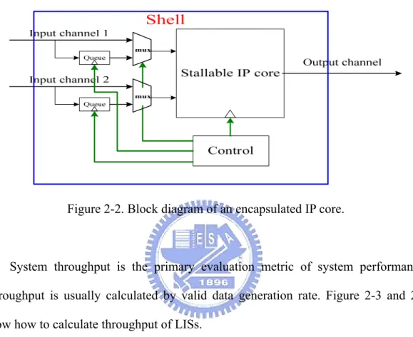
Figure 2-2 shows detailed architecture of encapsulated IP core. Block diagram in the example contains two input channels, one output channel, a controller to drive each element, and a stallable IP core. Each input channel has two end points. One is direct to input port of stallable IP core, and the other goes to the storage element queue located in every channel. IP core takes data either from input channel directly or from storage element controlled by multiplexer. A controller is accompanied with each encapsulated IP core, and it determines many vital controlling signals, such as select signal for multiplexer, stalling signal for IP core, and operation signals for queue. The details of the shell and relay station RTL logic designs are listed in [15]. Each shell and each relay station follow universal communication protocol. The protocol which allows shells and relay stations exchanging data on variant length channels is latency insensitive protocol (LIP) [11]. LIP defines the data exchanged by the shell as either valid or void and keeps the shells to ignore the existence of void data. The shell fires or executes the IP if and only if the IP can get a valid data from each input channel. The valid data from each input channel can be acquired from channel directly or from storage element queue. If the condition is not satisfied,

the shell stalls the core otherwise. The architecture of relay station is similar to the encapsulated IP. We can view the IP core of relay station as a simple edge triggered flip-flop.

Figure 2-2. Block diagram of an encapsulated IP core.

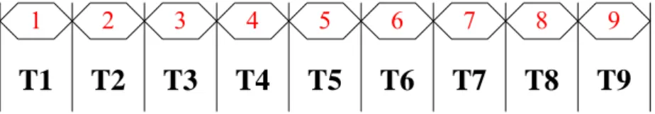
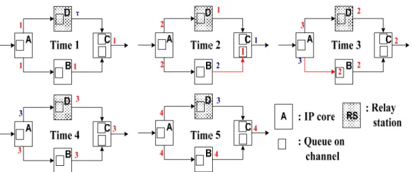
System throughput is the primary evaluation metric of system performance. Throughput is usually calculated by valid data generation rate. Figure 2-3 and 2-4 show how to calculate throughput of LISs.

1 2 3 4 5 6 7 8 9

T1

T2

T3

T4

T5

T6

T7

T8

T9

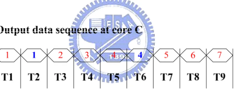
Figure 2-4. Output data sequence at core C in Figure 2-3.

In Figure 2-3, the big white rectangles represent IP cores in a system. The small white rectangles inside IP cores are queues on each input channel. IP A and B both have only one input channel and queue size on each input channel is all equal to 1. IP C has two input channels and queue size on each input channel is equal to 1, too. A channel queue, whose size is 1, is called a minimum queue so Figure 2-3 is an LIS with minimum queue on every channel. Red numbers in Figure 2-3 represent valid data and a positive integer “i” denotes the i-th valid data generated by the IP core. Note that when an IP core takes (i-1)-th valid data from its input channels, it outputs its i-th valid data to output channels if IP fires. Otherwise, a shell stores the valid data in queue when an IP stalls. We trace i-th valid data to get the valid data generation rate. This trace of data produced by IPs is called a progressive trace [16]. Since IP C is the only output of the simple LIS, system throughput can be derived by analyzing the data generation of output channel of IP C. Figure 2-4 shows the result of output data sequence at output channel of IP C. We find that IP C produces a valid data at every clock cycle so throughput of this LIS is 1 obviously. However, this simple LIS example does not consider the effect of inserted relay stations and back-pressure mentioned in [17] and [18]. A more realistic LIS example is showed in Figure 2-5. The shaded rectangle indicates a relay station and a relay station simply passes received data to its output channel at next clock cycle. Red numbers are valid data, the same definition as in Figure 2-3, and blue numbers mean void data. Since a relay station only passes the received data, it never generates new valid data. We assign a

symbol ‘τ’ to represent a non-generated and void data which a relay station outputs at timestamp 1.

Figure 2-5. Simple LIS example with inserted relay station and back-pressure.

In timestamp 1, all IP cores produce their first valid data, while relay station can only stall and release void data τ. In timestamp 2, IP C only receives a valid data from one of its input channel, but IP C needs two first valid data from each of its input channels to generate second valid data. Therefore, IP C stalls and outputs a void data. The first valid data generated by IP B is not processed, so it is stored in the queue of the lower input channel of IP C. As a result, lower input channel of IP C becomes full in the end of timestamp 2. In order to avoid valid data loss due to queue overflow, it forces IP B to stall at timestamp 3. The stop signal used to request source IP to stall at next timestamp is called back-pressure. The occurrence of back-pressure is highlighted by coloring the occurred channel red. In timestamp 3, IP C gets all required data from its input channels, so it can generate next valid data. IP B needs to stall, since the occurred back-pressure at timestamp 2. Note that since the queue of lower input channel of IP C is full at timestamp 2, the data sent by IP B at timestamp 2 will be discarded by the shell of IP C. This reason forces IP B to re-send generated

data at timestamp 3 although it stalls at timestamp 3. Another thing needed to be noticed is that the queue of IP B is full at timestamp 3. IP B sends a stop signal to IP A to request IP A to stall at next timestamp. In timestamp 4, all IPs produce their next valid data except IP A. IP A stalls at timestamp 4 but still re-sends data to IP B, like IP B does in timestamp 3. In timestamp 5, all IP cores fire to produce valid data and relay station passes a received void data. We find that the system behavior in timestamp 5 is identical to system behavior in timestamp 1. By progressive trace, we infer that the LIS example has a period of four clock cycles, as shown shows in Figure 2-6. Figure 2-6 is the output data sequence of IP C, and system behavior clearly repeats every four clock cycles. This LIS outputs three valid data in every four clock cycles, so throughput of LIS is obviously three fourth.

Figure 2-6. Output data sequence of core C in Figure 2-5

Finally, we summarize the advantages of LIS. LIS is a great solution to variant global interconnects length which is unknown in early design stage. By adding relay stations and encapsulating IP cores, LIS approach guarantees robustness for system behavior under LIP. However, LIS approach does not guarantee the same robustness for the throughput affected by back-pressure mechanism. There are two proposed technologies to deal with the throughput optimization problem of LIS. One is relay station insertion and the other is queue sizing of channel queue.

2.2 Throughput Optimization for Latency Insensitive System

The advantage and disadvantage of LIS have been discussed. Next, we discuss two related technologies used to optimize throughput of LIS.

2.2.1 Relay Station Insertion

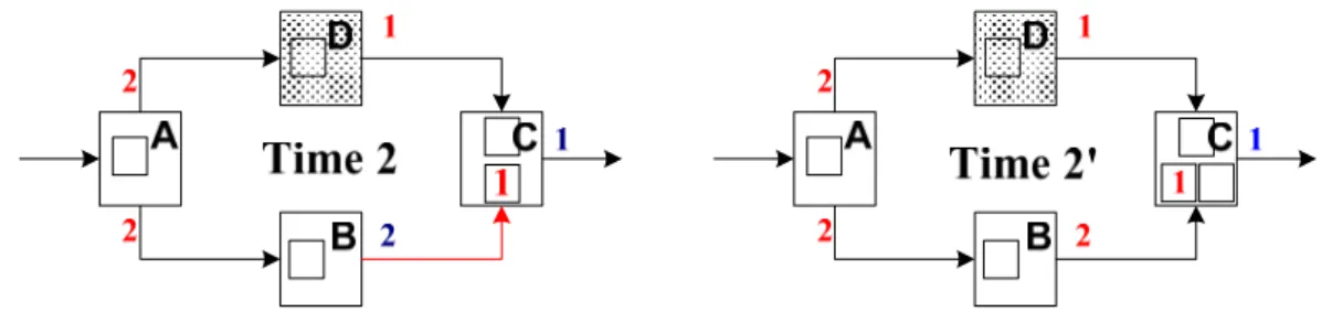
In Figure 2-5, we discover that one of the reasons cause the occurrence of back-pressure is the imbalance of channel latency. Data transmitted from IP A to IP C on upper path has experienced one clock delay but data transmitted on lower channel has not. The imbalance of channel latency results in occurrence of back-pressure and degrades throughput of LIS. Casu and Macchiarulo suggest equalization which basically equalizes all paths by inserting enough relay stations to make them have the same latency [19]. Therefore, there are two reasons that relay stations need to be added to an LIS. The first is to break up long channels to meet target clock period. The second reason is to optimize throughput by balancing latency of channels. Figure 2-7 demonstrates how to balance latency by inserting relay stations.

Figure 2-7. Optimize throughput by inserting relay station.

Left of Figure 2-7 is the same LIS example in Figure 2-5. We know that back-pressure occurs in this LIS architecture. Now, we insert a relay station to the channel connected IP B and IP C as shown in the right of Figure 2-7. As a result, all data arrived IP C have experienced the same latency, so back-pressure will not occur.

Throughput of the LIS improves to 1 finally. This is how we optimize throughput by relay station insertion. Nevertheless, relay station insertion still has its limitation. Lu and Koh have proved that equalization does not work for all systems [20]. Figure 2-8 illustrates a counter example. To balance the latency at paths from IP A to E a relay station must be added to either channel (A, C) or channel (C, E), but this ends up unbalancing either path from IP C to A or paths from IP E to C. Next, more relay stations need to be inserted to balance them. As a result, we find that throughput will never improve to 1 by doing exhaustive progressive trace.

Figure 2-8. Counter example of relay station insertion

From the discussed counter example, we know that relay station insertion still has some restrictions. Since relay station insertion is not a general solution for all LISs, the demand for better solutions rises.

2.2.2 Queue Sizing

Another reason which causes back-pressure to happen is size of queue. When queue is full, the shell needs to send a stop signal to stall source IP. This creates a motivation to increase size of queue so back-pressure will not happen. Without happening of back-pressure, performance of LIS can be optimized. Figure 2-9 illustrates the effect after increasing queue size of lower channel of IP C to 2. Left of

Figure 2-9 is the exact example in Figure 2-5 of timestamp 2. Back-pressure occurs when queue is full at this timestamp. After we adding one queue to lower channel of IP C, like the right of Figure 2-9, there always leaves one unused queue and hence back-pressure will never happen. Throughput of the example also improves to 1.

Figure 2-9. Optimize throughput by queue sizing

We view relay station insertion as another kind of queue sizing because relay station is a clocked storage element like queue. The difference of relay station and normal queue is that relay station forces all received data to delay one clock cycle but queue will not. The advantage of queue sizing is it will not potentially impact elsewhere in the system like relay station insertion since it only delays data by queue when needed. Increasing size of queue only causes slight additional hardware cost that will not influence whole system architecture in most of systems. Based on the characteristics, queue sizing becomes the mainstream of LIS throughput optimization. To be summarized, queue sizing offers a trade-off between performance optimization and area overhead.

2.3 Related Works

LIS has been discussed frequently in recent years. Many research works are made under different hardware architecture assumptions and different physical

information assumptions. Next, we are going to introduce two important research works on LIS topic. Earlier works before 2003 only considered ideal LISs (LISs with infinite queues and no back-pressure). Lu and Koh are the first people who proposed the method to solve LIS with back-pressure problem by queue sizing [17]. They showed that performance of a practical LIS with finite queues and back-pressure can reach the performance of an ideal LIS if proper queue sizing is adopted. They also proposed an approach to analyze complex LISs. Lis graph and extended lis graph were presented to model LISs. Throughput of an LIS was decided by the most critical cycles called the system cycles. Throughput calculation of those LISs has been shown in equation (1).

)

|

|

)

(

(

max

1

Ci

Ci

W

C Ci∈

−

₍₁₎

Where C is the set of all cycles in the lis graph. W(Ci) is the sum of edge weights of cycle Ci, and |Ci| is the number of edges in cycle Ci.

| | ) ( Ci Ci W

is called the cycle mean of cycle Ci. System cycles are cycles with max cycle mean and those cycles determine throughput upper bound. Throughput can not be further improved by queue sizing when it reaches throughput upper bound which is equal to 1 in most cases. Finally, Lu and Koh proposed a mixed integer linear programming (MILP) solution for queue sizing.

Collins and Carloni proposed a heuristic for queue sizing that produces solutions close to optimal solution in shorter time reported in [21] and [22]. A marked graph is a bipartite directed graph and Collins et al. use it to model LISs. Performance of LISs in marked graph is represented by maximal sustainable throughput (MST) θ. MST is determined by cycles with lowest tokens to places ratio. This ratio is similar to cycle

mean in [17]. The details of marked graph and MST will be introduced in Section 3.1. Token deficit problem (TDP) is the problem of filling the token (queue) deficit of cycles in an LIS. Collins et al. claimed that their heuristic algorithm for TDP is guaranteed to produce a performance-wise optimal solution that may require more queue space. Additionally, Collins et al. proposed two trends of LISs. One is that the position where relay station inserted affects throughput seriously. The other is the efficiency of fixed queue size. Collins et al. claimed that assigning every queue size to 5, and throughput is above 90% of the optimal solution. Collins et al. also make a different hardware architecture assumption with Lu et al. proposed in [17]. In our opinion, Collins’ hardware architecture assumption is closer to practical situation.

There are some different methods to solve LIS problem for different purposes. For instance, Casu and Macchiarulo avoided queue sizing issue by scheduling the activation of IPs [23]. A limitation of their work is that building schedules needs knowledge about the global system behavior. Bufistov et al. proposed the method that combines both queue sizing and relay station insertion techniques to achieve optimal throughput [24]. However, they made an assumption that the increase of queue size will also cause the increase of channel delay. This assumption will not happen in the hardware architecture we used.

Chapter 3

Throughput Optimization for LIS with Minimal

Buffer Size

3.1 Marked Graph and Quantitative Graph (QG)

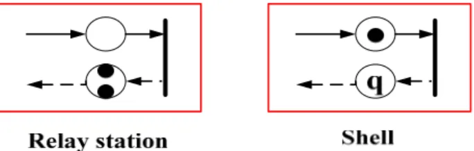
We introduce details of the marked graph first. Marked graph is a proposed modeling architecture for synchronous systems. Their simplicity makes them quite amenable to analyze synchronous systems which have a periodic behavior like LIS. A marked graph has two kinds of vertices: places and transitions. By definition, each place has exactly one incoming edge and one outgoing edge that both connect to transitions. Places have the ability to hold 0 or more tokens. Transitions cannot hold tokens, but they can fire and move tokens around in the graph. Each outgoing edge from a place connects to a transition, and each incoming edge connects to a place coming from a transition. A transition is enabled to fire when the place on each of its incoming edges has at least one token as the fire condition we described. All components of a marked graph fire to produce valid according to global clock. Detailed definitions of the marked graph are reported in [21], [22], and [25].

Figure 3-1. Modeling relay station and shell with marked graph representation.

The large white circles represent places, the small black circles represent tokens, the black vertical bars represent transitions, and the number q represents the channel has q tokens. Initially, the relay station’s place on solid edge has no token since the relay station produces a void data in timestamp 1, and its dashed edge has two tokens on place corresponding to the two available storage spaces in the queue. Recall that relay station is a clocked buffer with two storage capacity. The shell’s place on solid edge has one token since the shell produces a valid data in timestamp 1, and its dashed edge has q tokens on place. Number q is a positive integer. Using a marked graph representation, valid or void data are presented by tokens on the solid edges. The tokens on the dashed edges represent available spaces of queue in the channel [21].

Figure 3-2. Transformation from original LIS graph to marked graph representation.

Figure 3-2 illustrates how to transform original LIS graph to a marked graph representation. All queue size of shells are set to 1 in this case. It is convenient to calculate MST after we transform LIS to marked graph. We used to compute system throughput by progressive trace as mentioned in Section 2.1, but progressive trace spends a lot of time to simulate IP behavior on every timestamp, so it is unpractical to calculate throughput by progressive trace in complex system. However, based on Section 2.3, we can compute the MST of the graph by finding the cycles with the lowest ratio of tokens to places. In Figure 3-2, the most critical cycle {A, D, C, B, A} has four places but only three tokens on it, so the system has MST of three fourth.

Another convenience of marked graph representation is that it can reflect queue sizing problem easily. Figure 3-3 shows how to reflect queue sizing problem to the marked graph. If we want to add an extra queue to IP B, we only need to put an additional token on dashed edge of IP B. Finally, the most critical cycle {A, D, C, B, A} of the system has ratio equal to 1, so the system has optimal MST 1.

Figure 3-3. Queue sizing problem reflects to marked graph representation.

We prefer to adopt marked graph representation on our LIS research. This is because: (1) it is easy to transform original LIS graph to marked graph representation. All we need to do is to find all channels and IP cores in LIS, and then transforms them to relay station or shell representation, as shown in Figure 3-1. (2) throughput of LIS is easy to calculate in marked graph, since we only need to find the cycles with lowest tokens to places ratio in the marked graph. (3) it is easy to decide which places in the marked graph should have more tokens. This greatly helps us find the optimal solution.

Although marked graph representation is convenient, there still exist some drawbacks in it. One is that we used to calculate throughput with pure integer number. Using tokens and places is easy to operate at graph, but it is indirect in calculating throughput. Since that, we propose a new graph representation quantitative graph (QG)

which can handle those problems properly. Figure 3-4 shows the flow how we transform from a marked graph to a quantitative graph. First, we want to quantify number of places and tokens into integers. Now we get an intermediate graph which only contains four integers in each channel. Second, we transform every transition into a vertex and get rid of all dashed edges in the intermediate graph. This is feasible because each dashed edge corresponds to a solid edge in the marked graph. Whenever there exists a solid edge, there must exists a corresponding dashed edge. In the end, we create a new graph with vertices and four weightings in each channel. Those weightings represent number of places and tokens on solid edge and dashed edge of the channel. We call this new graph quantitative graph.

A D B C (1,0) (1,2) (1,1) (1,1) (1,1) (1,1) (1,1) (1,1)

A

D

B

C

[1,0,1,2] [1,1,1,1] [1,1,1,1] [1,1,1,1] ● ● ● ● ● ● ● ● A D B C (ps, ts) (pd, td)

ps(e) : places of solid edge ts(e) : tokens of solid edge pd(e) : places of dashed edge

td(e) : tokens of dashed edge [ps(e), ts(e), pd(e), td(e)]

Figure 3-4. Transformation from a marked graph to a quantitative graph.

Definition of quantitative graph: A quantitative graph GQ = (VQ, EQ, ps, ts, pd, td)

is a weighted directed graph, where ‧ VQ is the set of vertices.

‧ ps: E→Z+ shows the number of places of the corresponding solid edge. ‧ ts: E→N represents the number of tokens of the corresponding solid edge. ‧ pd: E→Z+ identifies the number of places of the corresponding dashed edge. ‧ td: E→Z+ is the number of tokens of the corresponding dashed edge.

Formal transformation from a specified marked graph to the quantitative graph is described as follows. Each transition ti in the marked graph converts to a vertex vi in

the quantitative graph. Each edge (vi,vj) in the quantitative graph corresponds to a pair

of edges in the marked graph, including a solid edge (ti,tj) and a dashed edge (tj,ti).

Places and tokens of solid edges transform to weightings ps and ts in the quantitative graph. Places and tokens of dashed edges transform to weightings pd and td. For example, ps((vi, vj))=1, ts((vi, vj))=0, pd((vj, vi))=1, and td((vj, vi))=2 represent an

input channel of relay station in the quantitative graph. System throughput of QG is decided by cycles with lowest ratio of tokens to places, which is identical to original marked graph. However, tokens and places in the marked graph are transformed to weightings in the quantitative graph. Throughput calculation of QG is modified to find lowest ratio of

∑

∑

∑

∑

∩ ∈ ∩ ∈ ∩ ∈ ∩ ∈ + + D C e S C e D C e S C e e pd e ps e td e ts( ) ( ) ( ) ( ) in the graph.

Summation of ts and td represent total tokens in cycle C. Summation of ps and pd are total places in cycle C. S represent set of solid edges and D represent set of dashed edges. We define this ratio as T(C).

3.2 Quantitative Graph Reduction

There still exist some vital problems unsolved even after we transform marked graph to QG. One of them is when global interconnects latency becomes worse, and we will need more relay stations to pipeline interconnects, so graph size becomes

huge. Some LISs may be unsolvable due to huge graph size. That urges us to try to further reduce graph size.

3.2.1 Path Condensation

If there exists a simple path in the QG and every vertex inside the path all have only one input edge and only one output edge. We find that it is equivalent in calculating throughput after we combine all edges and vertices in the simple path into a single edge. And all weightings of the single edge are the summation of weightings of all combined edges.

Figure 3-5. Two graphs are equivalent in throughput calculation.

Figure 3-5 illustrates the concept of combination. Left graph of Figure 3-5 is original QG and right graph of Figure 3-5 is the graph after combinative operation. The pink vertex represents relay station and the two red edges correspond to two combinative paths in the left graph. Left graph has two cycles when we consider solid edges only. T(C) of those two cycles are two third and one. Since system throughput is determined by cycles with lowest T(C), system throughput of left graph is two third finally. Right graph also has two cycles with T(C) equals two third and one. System throughput of right graph is also two third. In the end, two graphs are equivalent in

system throughput but right graph has fewer vertices and edges. In other words, right graph is more efficient in counting cycles in the graph, this is to say, more efficient in calculating system throughput. We define this combinative operation as path condensation. By path condensation operation, we can eliminate all the relay stations and some IPs in the QG without influencing system throughput.

Definition of path condensation: We call a simple path pu,v <u,v1,…vn,v>

condensable if the path satisfies the following two conditions. ‧ The length of path |pu,v|≥ 3, or n ≥ 1

‧ For each intermediate vertex {v1,v2,…,vn}, its input degree and output degree

must both equal to 1

Each condensable path pu,v can be replaced by a condensed edge ec (u, v) without

affecting the overall system throughput, and for each condensed edge ps(ec)=pd(ec)=n+1, ts(ec)=

∑

∈ ( ,) ) ( v u p E e e ts , td(ec)=

∑

∈ ( _, ) ) ( v u p E e e

td . E(pu,v) is the set of edges

belonging to condensable path pu,v,, that is (u, v1), (v1, v2)…...(vn, v).

3.2.2 Edge Unification

After we doing path condensation operation, we find the rest graph can be further reduced in number of edges. We observe that one of two red edges is dominating in calculating throughput in Figure 3-5. We observe left of Figure 3-6, and we know system throughput is two third. In other words, the cycle contains upper red edge dominating system throughput. That is to say, we can eliminate the other one red edge without affecting correctness of throughput calculation. The activity is showed in right of Figure 3-6 which dominating edge is kept and the other is eliminated. We

define this operation as edge unification. v1 v3 [1,1,1,1] [2,1,2,3] v1 v3 [1,1,1,1] [2,1,2,3] [2,2,2,2]

System throughput : 2/3 System throughput : 2/3

Figure 3-6. Operation of edge unification.

Definition of edge unification: For any two vertices vi, vj in the quantitative

graph, if there exist multiple edges from vi to vj, we group those edges into an

Em. Each Em can be unified into a dominating edge ed, and we keep the

dominating edge and get rid of others edges belonging to the same Em. This

unification maintains system throughput. Each dominating edge ed is the edge

with max(ps(e)-ts(e)), where e∈Em.

In Figure 3-6, the graph has only one Em which contains two red edges. From the

definition, we know that upper red edge is the dominating edge of Em, so we eliminate

the lower edge to decrease number of cycles in the graph. By edge unification, QG can de further reduced on graph size. Figure 3-7 demonstrates an example of total reduction procedure.

Figure 3-7. Total reduction procedure of an LIS example.

Figure 3-7 starts from a marked graph with seven channels where size of queue need to be decided. Those variables are indexed as a1 to a7. This is because queue size

of the relay station is fixed to 2 in marked graph. Marked graph make this assumption to keep the relay station small and consistent. Therefore, we only need to view size of queue in each shell as a variable. In other words, now we have seven variables in this example. Next, we transform marked graph representation to QG representation. Then, we do the reduction procedure to the QG. From the definition of path condensation and edge unification, we know those procedures will not affect correctness of throughput. Finally we acquire a reduced graph which has the same throughput with the original marked graph while eliminating variables from seven to three. This makes throughput calculation in the reduced graph faster than with initial marked graph. After getting result of system throughput, we need to recover from reduced graph to original QG to get the correct number of queues in whole system. We show this recovered procedure in Figure 3-8 and Figure 3-9.

Figure 3-8. An example of recovered procedure step 1 v1 v2 r1 v3 v4 [1,1,1,2] [1,0,1,2] [1,1,1,2] [1,1,1,2] r2 [1,0,1,2] r3 [1,1,1,3] v6 [1,0,1,2] [1,1,1,1] v5 [1,1,1,3] [1,1,1,3] v1 v4 [4,3,4,8] v6 [3,1,3,7] [1,1,1,1] [2,2,2,6] Recover_2

Figure 3-9. An example recovered procedure step 2.

In Figure 3-8, we illustrate recovered procedure step 1. In step 1, we recover reduced graph from edge unification first. To maintain the optimal throughput in recovered procedure, there is a condition must be satisfied. The condition is to make all edges belong to the same Em have equal td(e)-pd(e). That is to say, for all e∈Em,

we make their td(e)-pd(e) equal. This is because all e∈Em needs to have the same

number of extra queues. Whenever a cycle passes throughput the dominating edge of Em, there must exist other cycles pass throughput other edges belonging to the same

Em in the original QG. When the cycle passes throughput dominating edge needs extra

queues to achieve optimal throughput, we infer that other edges belonging to the same Em will also need the same number of extra queues to maintain optimal throughput.

For instance, we assign td(e) of the dominating edge in left of Figure 3-8 to be 8. Then, we know td(e) of the other one edge is equal to 6, since 8-4 = 6-2. In step 2, we recover reduced graph from path condensation as showed in Figure 3-9. We already know that queue size of relay station is fixed to 2 so we only need to distribute rest queues to the shells equally. For instance, a condensed edge with 6 queues in the left of Figure 3-9 is recovered into corresponding two edges (v1, v5) and (v5, v4) in the

right of Figure 3-9. Each edge is allotted with 3 queues. We distribute queues equally in order to make every shell with similar area in hardware. As a result, we acquire final correct queue size solution in right of Figure 3-9.

3.3 Problem Formulation of Our approach

By the path condensation and edge unification, we can decrease graph size extremely and still keep the correctness of system throughput. It helps a lot in counting cycles in the graph for throughput calculation. Hence, we can find the optimal throughput quickly with the reduced QG. Then we propose an integer linear programming (ILP) to find the minimal queue size while maintaining optimal throughput. Following are proposed problem formulation:

Given:

‧ A quantitative graph GQ(VQ, EQ, ps, ts, pd, td).

Objective :

‧ Minimize total queues

∑

∈EQ

e

e

td( while maintaining maximum throughput. )

Constraints :

‧ For each cycle C, ( )=(

∑

( )+

∑

( )

∑

( )+

∑

( ))≥1

∩ ∈ ∩ ∈ ∩ ∈ ∩ ∈C S e C D e C S e C D e e pd e ps e td e ts C T ,

where S represents set of solid edges and D represents set of dashed edges.

The proposed ILP formulation for the minimal queue size is very efficient because it has only |E| integer variables, and |C| constraints. |C| is number of cycles. The flow of our approach is separate into three main processes that are discussed as following:

constructing graphs from the benchmark, assigning the length latency of each channel, reducing graph size by path condensation and edge unification. All works make the graph can be handled easily and faster. 2. Find cycles: In this process, we identify all the cycles in the graph. By the

helping of reduction procedure, cycles in the graph will be decreased greatly. Hence, the time spent in this process will be shortened greatly, too. We use Johnson’s algorithm [26] to help us to find all the cycles in the graph.

3. ILP process: This is the main process of our approach. We take cycles obtained from process 2. And for each cycle, we decide queue size of each shell to make all cycles’ T(C) bigger or equal to 1 while minimizing total queue size.

3.4 Bit Width of Channels

In practical SoC system, channels usually have bit width on them. For example, a 32-bit CPU may has 32, 16, and 1-bit channels on it. Therefore, we take channel bit width issue into consideration. In LISs, queues are put to different positions will make different area cost when bit width is considered. Figure 3-10 illustrates the different area costs are made by different queues added positions.

To take bit width of channels into consideration, we only need to modify our graph representation slightly. We add an extra width weighting w(e) to every edge in the QG. In other words, we modify four weightings (ps(e), ts(e), pd(e), td(e)) in each edge into five weightings (ps(e), ts(e), pd(e), td(e), w(e)). Since our purpose is to maintain optimal throughput with minimal queue size, the reduction procedure and formulations need to be changed for consistency of system throughput. For path condensation, ps, ts, pd, td are still the same like in Section 3.2, and w(e) is assigned to minimal width among the edges of condensable path. This is because we prefer to put queues in edges with lower bit width to achieve minimal queue size. For edge unification, ps, ts, pd, td of dominating edge are still the same like in Section 3.2, and w(e) is assigned to summation of w(e) of all edges belong to the same Em. This is

because we need to let all e∈Em have equal extra queues. Whenever the dominating

edge needs an extra queue, other edges belonging to the same Em will need an extra

queue, too. Figure 3-11 shows the changes in path condensation and edge unification. In upper graphs of Figure 3-11, w(e) of condensed edge is the smaller w(e) of edge of condensable path <v1, v4>. In lower graphs in Figure 3-11, w(e) of dominating edge is

the w(e) summation of two edges from v1 to v4.

Some changes are made to our proposed ILP formulation. The modified formulation show as follows:

Given:

‧ A quantitative graph GQ(VQ, EQ, ps, ts, pd, td, w).

Objective :

‧ Minimize total queue

∑

∈ × Q E e e w e

td( ) ( ) while maintaining maximum

throughput. Constraints :

‧ For each cycle C, ( )=(

∑

( )+

∑

( )

∑

( )+

∑

( ))≥1

∩ ∈ ∩ ∈ ∩ ∈ ∩ ∈C S e C D e C S e C D e e pd e ps e td e ts C T ,

where S represents set of solid edges and D represents set of dashed edges.

We only slightly modify objective function of our ILP formulation in Section 3.3. It is easy to take bit width issue into consideration on our graph representation and ILP formulation. This makes our proposed graph representation and formulation useful among the system with bit width all equal to 1 or the system with different bit width.

Chapter 4

Experimental

Results

4.1 Environment Setup and Benchmarks

The benchmarks we used contain three sets, MCNC, GSRC, and ISCAS89. However, MCNC and GSRC lack of transfer direction information. In order to add data dependency between the IPs in each benchmarks, we break each net on those benchmarks into a 2-pin net and randomly assign it with a direction. To provide more realistic cases, we take two cases of ISCAS89 as another benchmark set. Those ISCAS89 benchmarks already have direction information. The experiments are processed on a computer with an AMD 1.81GHz CPU and 2GB DRAM. We use the non-commercial LP/ILP solver lp_solver [27] to solve the proposed ILP formulation. Figure 4-1 shows the flowchart of our experiments.

4.2 Weight and Channel Latency Assignment

Since latency of each channel is generated randomly in our experiments, more precisely, channel latency is a random real number obtained from an interval [1, A]. In other words, 0~A-1 relay stations are inserted to pipeline channel into 1~A parts. For example, if the random generated number is 2.4, it means that data need 2.4 clock cycles to transmit data along the channel, and two relay stations need to be inserted. Each relay station in the experiments has 2 fixed queues like mentioned in Section 3.2. The queue size of each shell is assigned to be one initially.

The bit width of each channel in a benchmark is assigned to be one initially. This means that each channel is a one-bit communication channel. To test the influence of bit width on channels, we assign a set of different bit width to channels. Then we compare the difference between those two bit width assignments. To model the worst case of benchmarks, we assume that every benchmark can achieve optimal throughput 1. This is the worst case because we need to consider every cycle and make its T(C) bigger or equal to 1 when throughput upper bound is 1. If throughput is a real number smaller than 1, cycles with tokens to places ratio bigger than throughput upper bound can be omitted.

4.3 Results

For each benchmark, we make three experiments on it. We find the efficiency of the reduction procedure in experiment Ⅰ. In other words, how many cycles are omitted after path condensation and edge unification are performed. In experiment Ⅱ, we compare our approach and heuristic algorithm proposed in [21] and we verify the variation when channel latency becomes worse. Finally, we compare our approach

and heuristic algorithm when bit width issue is considered.

4.3.1 Experiment Ⅰ

In experiment Ⅰ, we count number of cycles in original marked graph and in reduced QG. We use Johnson’s algorithm [26] to help us to count all cycles in both two graph representations. Channel latency locates on interval [1, 3]. In other words, 0~2 vertices are added to every edge in graphs.

Table 4-1. Number of cycles degradation after the reduction procedure performed. Original QG Reduced QG

Benchmark

Set Case Name (V,E) # Cycles (V,E) # Cycles apte (30,45) 2965 (7,16) 350 xeorx (31,40) 357 (8,15) 193 hp (28,33) 66 (10,13) 37 ami33 (82,99) 8962 (29,44) 7782 MCNC ami49 (172,314) * (17,49) 234972 n10 (27,34) 2468 (7,14) 176 n30 (76,97) 137647 (21,39) 16512 n50 (107,146) * (29,50) 29926 n100 (184,207) * (64,74) 10583 n200 (301,327) * (128,135) 19169 GSRC n300 (482,636) * (122,183) 38443 s344 (297,397) 96588 (44,61) 488 ISCAS89 s349 (299,402) 74713 (44,61) 404

From Table 4-1, we show five MCNC benchmarks, six GSRC benchmarks, and two ISCAS89 benchmarks. Each Benchmark’s name and its experimental results are listed in Table 4-1. Column (V, E) under marked graph represents vertices and edges in original marked graph. Column # Cycles under marked graph represents number of cycles in marked graph representation. Column (V, E) and # Cycles under reduced

QG have the same meaning with definitions under marked graph. * represents number of cycles exceed one million so that is too hard to solve problem with this size. The reduction procedure decreases graph size from unsolvable to solvable size in one of five benchmarks of MCNC. And it decreases four benchmarks of GSRC to solvable size. We make the conclusion that reduction procedure is useful in decreasing cycles in the graph.

4.3.2 Experiment Ⅱ

In experiment Ⅱ, we verify the difference between our proposed method and Collins’ method in [21]. We make two different set of channel latency assignments in two experiments in experiment Ⅱ. The results of channel latency located on [1, 3] are showed in Table 4-2. The results of channel latency located on [1, 5] are showed in Table 4-3. All bit width is assigned to 1 in experiment Ⅱ.

Table 4-2. Experimental results when channel latency locates on [1, 3]. Proposed Method Collins Method Benchmark

Set Case Name # Queues Run Time(s) # Queues Run Time(s)

apte 19 0 27 0 xeorx 43 0 43 0 hp 19 0 19 0 ami33 41 1 61 1 MCNC ami49 520 747 548 319 n10 14 1 17 0 n30 57 6 74 2 n50 58 23 87 7 n100 85 4 104 2 n200 101 12 150 5 GSRC n300 182 54 241 24 s344 95 0 116 0 ISCAS89 s349 107 0 132 0 Ratio 1 1 1.22 0.42

From Table 4-2, we show the experimental results of two methods. Column # Queues represents number of queues needed to maintain optimal throughput in our proposed method and in Collins’ method. Run time represents time needed to compute this solution. Run time is counted by seconds. Our method saves 22% number of queues than Collins’ method on average, but run time of our method is 2.5 times than Collins’ method on average.

Table 4-3. Experimental results when channel latency locates on [1, 5]. Proposed Method Collins Method Benchmark

Set Case Name # Queues Run Time # Queues Run Time

apte 67 0 67 0 xeorx 35 0 37 0 hp 15 0 15 0 ami33 85 1 151 1 MCNC ami49 618 947 691 371 n10 38 1 44 0 n30 92 7 105 2 n50 167 35 242 10 n100 126 5 142 2 n200 149 18 261 7 GSRC n300 459 73 545 31 s344 182 0 240 0 ISCAS89 s349 142 1 184 0 Ratio 1 1 1.25 0.39

Our method saves 25% number of queues than Collins’ method on average, but run time of our method is still about 2.5 times than Collins’ method in Table 4-3. Compared Table 4-2 and 4-3, we find when the channel latency becomes worse, the difference between Collins’ method and our method enlarge. Our method will perform better than pervious works when channel latency becomes worse. From Chapter 1, we know that channel latency becomes worse as the manufacturing process scales down.

To be summarized, our method offers smaller area cost than Collins’ method with acceptable extra time.

4.3.3 Experiment Ⅲ

In experiment Ⅲ, we verify the difference between our method and Collins’ method when bit width is considered. Channel latency is limited to interval [1, 3]. Bit width of channels is assigned to 8, 16, 32, and 64 randomly. Those bit numbers are common used in practical chips.

Table 4-4. Bit width is assigned to 8, 16, 32, and 64 randomly.

Proposed Method Collins Method Case Name # Queues Run Time # Queues Run Time

apte 816 1 1176 0 xeorx 1048 0 1048 0 hp 640 0 832 0 ami33 968 2 1768 1 MCNC ami49 14192 782 15568 327 n10 472 0 568 0 n30 1296 6 2192 2 n50 1360 23 2344 7 n100 3136 3 4320 2 n200 2000 13 4072 4 GSRC n300 5216 56 7256 25 s344 3384 0 4664 0 ISCAS89 s349 3104 0 4400 1 Ratio 1 1 1.33 0.41

From Table 4-4, our method saves 33% number of queues than Collins’ method on average, but run time of our method is still about 2.5 times than Collins’ method. Compared the experimental results in Table 4-2, which channel latency is assigned to

1, the difference between our method and Collins’ method enlarge greatly after taking bit width issue into consideration. To be summarized, our method offers better area cost than Collins’ method in more practical circuits.

4.4 Discussion

In experiment Ⅰ, our proposed reduction procedure is efficient in decreasing number of cycles in the graph. Since the number of cycles in a directed graph can grow faster than the exponential 2n, it is important to reduce the graph size of practical circuits. Without the reduction procedure, we know from Table 4-1 that cycles in some benchmarks exceed one million. The million order cycles are hard to process in normal computers and waste time to count all cycles. This is why reduction procedure is so important.

In experiment Ⅱ, our proposed method saves 22% of queues than Collins’ method on average. Even our method cost about 2.5 times on run time than Collins’ method, but additional time cost in our method is still acceptable. For instance, the benchmark with the most cycles in our experiment, ami49, only cost 947 seconds to solve it. So, we usually prefer to sacrifice acceptable time but saving valuable area in the chips. We make another experiment to verify what will happen if channel latency becomes worse. The experimental results show our method is more suitable than Collins’ method in worse channel latency.

In experiment Ⅲ, our proposed method saves 33% of queues than Collins’ method on average if bit width is considered. With similar time overhead to experimental results showed in Table 4-2, our method saves more area than Collins’

method when bit width is considered. The similar run time is because the only difference between those two formulations is the objective function. This makes our method more elastic to transform between different bit width assignments.

Since number of cycles determines efficiency of our method, decreasing number of cycles is the vital problem for our method. We propose the reduction procedure including path condensation and edge unification to decrease number of cycles. However, there are some experimental skills helping us further reduce number of cycles. One is to ignore the cycle if and only if its T(C)>1, since it is not the most critical cycle. Another is to collapse each strongly connected component (SCC) into a single vertex. This is because throughput upper bound in our experiment is 1, and each sub-system must finally have throughput 1, too. Hence, we can view each SCC as a sub-system with throughput 1, and then we collapse them into a single vertex. The final one is to ignore cycles containing only two edges, since it must the self-loop cycle in the original marked graph.

Chapter 5

Future Works and Conclusions

As the manufacturing process to deep submicron technology, length of interconnects becomes more unpredictable and uncontrollable. It makes designers hard to assembly pre-designed IP cores together at early design stage since the unknown signal transference time. Repeater insertion is the promising solution to solve this problem without heavily changing the designs. However, slight modifications on existed IP cores are unavoidable. This prolongs the product developed period on meaningless modification. And even worse, repeater insertion will degrade performance of overall system by multi-clock communication. LIS is a good solution for those existed problems. LIS handle the unpredictable interconnects problem by automatic inserting relay stations which is similar to mentioned repeater insertion. LIS avoids modified iterations by encapsulating every existed IP cores. Encapsulating is to add some additional hardware called shell to the existed IPs. This step makes all encapsulated IP cores and relay stations can follow the same communication protocol—latency insensitive protocol. LIS works out performance degradation mainly by queue sizing technology. Finally, product developed period shortens and company can earn more benefit. From those reasons, we know that LIS is a gorgeous solution for time-to-market. However, the physical parameters, like length of interconnects, positions of IPs…etc. are known after floorplanning performing. From Section 2.1, we know throughput upper bound of an LIS is determined by system architecture. In other words, poor system architecture limits the spaces that LIS can improve. In our experimental results, channel latency is assigned to a reasonable interval, not obtained from realist floorplanning results. There are

many research working on determining best system architecture on floorplanning stage reported in [28] and [29]. After those performance-aware floorplannng performing, we acquire real physical information which is closer to optimal architecture. So our future direction is to combine our proposed method with real physical information acquired from performance-wise floorplanning.

We propose an optimal throughput optimization technique for LIS with minimal queue size. First, we transform original marked graph to quantitative graph. Then, we develop the reduction procedure for graph size reduction. We use an ILP formulation to guarantee the minimal queue demand. After acquiring minimal queue solution from reduced quantitative graph, we develop a recovered procedure to transform reduced quantitative graph back to quantitative graph while maintaining correctness of minimal queue size. The experimental results show that our method outperforms Collins’ in terms of queue size (area cost). Runtime of our method is acceptable for real industrial systems.

References

[1] R. H. Havemann and J. A. Hutchby, “High-performance interconnects: an integration overview,” in Proceedings of IEEE, pp. 586–601, 2001.

[2] R. Ho, K. W. Mai and M.A. Horowitz, “The future of wires,” in Proceedings of

IEEE, pp. 490–504, 2001.

[3] International Technology Roadmap for Semiconductors, Semiconductor Industry Association, 2005.

[4] D. M. Chapiro, “Globally-asynchronous locally-synchronous systems,” Ph.D. dissertation, Stanford Univ., CA, 1984.

[5] D. S. Bormann and P. Y. Cheung, “Asynchronous wrapper for heterogeneous systems,” in Proc. ICCD, pp. 307–317, 1997.

[6] J. Muttersbach, T. Villiger and W. Fichtner, “Practical design of globally-asynchronous locally-synchronous systems,” in Proc. ASYNC, pp. 52–59, 2000.

[7] S. Kumar, A. Jantsch, J-P. Soininen, M. Forsell, M. Millberg, J. Oberg, K. Tiensyrja, and A. Hemani, “A network on chip architecture and design methodology,” in Proc Symposium on VLSI, pp. 117–124, 2002.

[8] A. Hemani, A. Jantsch, S. Kumar, A. Postula, J. Oberg, M. Millberg, and D. Lindqvist, “Network on a chip: an architecture for billion transistor era,” in Proc.

of the IEEE NorChip Conf., 2002.

[9] J. Cong, Y. Fan, G. Han, X, Yang, and Z. Zhang, “Architecture and synthesis for on-chip multicycle communication,” in Proc. TCAD, pp. 550–564, 2004.

[10] J. Cong, Y. Fan, Z. Zhang, “Architecture-level synthesis for automatic interconnect pipelining,” in Proc. DAC, pp. 602–607, 2004.

[11] L. P. Carloni, K. L. McMillan, and A.L. Sangiovanni-Vincentelli, “Latency-insensitive protocols,” in Proc. of the Computer-Aided Verification

(CAV), 1999.

[12] L. P. Carloni, K. L. McMillan, and A.L. Sangiovanni-Vincentelli, “Theory of latency-insensitive design,” in IEEE Tran. CAD, vol. 20, no. 9, 2001.

[13] V. Adler, E. G. Friedman, “Repeater design to reduce delay and power in resistive interconnect,” in IEEE Trans. Circuits Syst. II: Analog Digital Signal

Process, vol. 45, no. 5, pp. 607–616, 1998.

[14] L. P. Carloni, K. L. McMillan, A. Saldanha, and A. L. Sangiovanni-Vincentelli, “A methodology for correct-by-construction latency insensitive design,” in Proc.

ICCAD, pp. 309–315, 1999.

[15] C. Li, R. Collins, S. Sonalkar, and L. P. Carloni, “Design, implementation, and validation of a new class of interface circuits for latency insensitive design,” in

Fifth ACM-IEEE International Conference on Formal Methods and Models for Codesign (MEMOCODE), 2007.

[16] L. P. Carloni and A. L. Sangiovanni-Vincentelli, “Performance analysis and optimization of latency insensitive systems,” in Proc. DAC, pp. 361–367, 2000. [17] R. Lu, and C. Koh, “Performance optimization of latency insensitive systems

through buffer queue sizing of communication channels,” in Proc. ICCAD, pp. 207–231, 2003.

[18] L. P. Carloni, “The role of back-pressure in implementing latency-insensitive systems,” in Electronic Notes in Theoretical Computer Science (ENTCS), vol. 146, no. 2, 2006.

[19] M. R. Casu and L. Macchiarulo, “Issues in implementing latency insensitive protocols,” in Proc. of the Conf. on Design, Automation and Test in Europe, pp. 1390–1391, 2004.