Sharing of multiple images: economically sized and fast-decoding approach based on modulus and Boolean operations

Sharing of multiple images: economically sized

and fast-decoding approach based on

modulus and Boolean operations

Kun-Yuan Chao Ja-Chen Lin

National Chiao Tung University

Department of Computer and Information Science 1001 Ta Hsueh Road

Hsinchu, 300 Taiwan

E-mail: kychao@cis.nctu.edu.tw

Abstract. Secret image sharing is a popular technology to secure digital images in storage and transmission. Traditionally, the technology trans-forms one secret image into several images called shadows or shares. Later, when the number of collected shadows reaches a specified threshold value, the decomposed image can be reconstructed. We pro-pose a new sharing approach to transform n secret images into n shad-ows. Later, after gathering all the n shadows, all the n secret images can be retrieved error-free. No information in any secret image is revealed if one shadow is absent. The total size of n generated shadows is identical to the total size of n input secret images; hence, this approach does not waste storage space. Each pixel in each secret image is reconstructed using only one Boolean, one modulus, and two mathematical operations, so it is also a fast approach for reconstructing many secret images. Comparisons are included. © 2010 Society of Photo-Optical Instrumentation

Engineers. 关DOI: 10.1117/1.3407067兴

Subject terms: multi-image sharing; modulus operation; Boolean operation; input/ output size ratio; computational complexity.

Paper 090756R received Sep. 28, 2009; revised manuscript received Feb. 6, 2010; accepted for publication Mar. 1, 2010; published online Apr. 20, 2010.

1 Introduction

To secure an image file in storage or transmission, there are two well-known sharing approaches: polynomial secret sharing 共PSS兲1 and visual cryptography 共VC兲.2 They can divide a secret image into several extremely noisy images called shadows 共also called shares兲. Each participant can hold some of these shadows. Later, when the total number of shadows brought to a meeting reaches a specified thresh-old value, the shared secret image can be reconstructed. Several extended works of the introducing papers1,2 have been reported. Examples include the reduction of memory cost for shadows,3extension of binary VC to grayscale4or color images,5 even a two-in-one sharing method called VCPSS6that combined PSS and VC to create a tool whose decoding quality depends on the condition of whether a computer is available or not.

In real life, a project team often processes several secret images simultaneously. Therefore, some research shared multiple images in one encoding process. For example, the elegant PSS scheme7 presented by Feng et al. used Lagrange interpolation to deal with multisecret images. Their method is an economical method, for it has a very high input/output共I/O兲 size ratio between 1/2 and 1, i.e., total input image size is at least 50% of the total output shadow size, and 100% is possible. But the computational complexity O共log2_{k兲 would be needed to reconstruct each} secret pixel by using Lagrange interpolation from k re-quired shadows. To the contrary, to save computational op-erations in the retrieval of secret images, visual

cryptogra-phy 共VC兲 schemes can be used. For example, Shyu et al. used two circular shadows to design a VC scheme8that can share more than two secret images. Feng et al. also pre-sented a multisecret VC scheme,9and their shadows are in rectangular shape. By stacking the shadows共know as trans-parencies in the VC field兲, these VC schemes are very fast in revealing all secret images. The disadvantage of using VC methods is their low I/O size ratio共at least 1/2兲 due to the high pixel expansion rate共per⭌2兲 in generating shad-ows. As for the disadvantage of the low contrast of the images recovered by stacking transparencies, it can be avoided if VC methods are implemented on a computer. When VC methods are implemented on a computer to re-construct n original secret images error-free, the complexity to decode a pixel of a secret image would be O共n兲 due to the high per.

Besides PSS and VC schemes, Alvarez, Encinas, and del Rey also developed a multisecret sharing scheme10 for color images with different sizes based on modulus opera-tions. Albeit their I/O size ratio is a very good value n/共n + 1兲 after sharing n secret images by n+1 shadows, their reconstruction in each secret pixel needs one modulus op-eration and many mathematical opop-erations共addition or sub-traction兲 whose computational complexity is O共n兲. Muñoz-Rodríguez and Muñoz-Rodríguez-Vera developed three very fast methods11–13 based on phase encoding of a secret image and a pattern image. In their methods, decoding is per-formed by using just a simple overlapping operation to re-trieve each pixel of the input secret image. The methods are very fast, but their decryption creates approximated ver-sions of the original image, rather than error-free recovery. Among the error-free 共lossless兲 schemes7–10 for multise-0091-3286/2010/$25.00 © 2010 SPIE

crets, no one can simultaneously own the two advantages: 1. I/O size ratio is 1, and 2. only a constant number of operations is needed to reconstruct each secret pixel. To achieve these two advantages simultaneously, we propose here a novel sharing scheme for multiple images, by using modulus共MOD兲 and exclusive-OR 共XOR兲 operations. The proposed method generates n extremely noisy shadows for

n given binary/grayscale/color secret images共notably, the n

given images all have the same size兲, and each shadow’s size is identical to each given image. When the n shadows replace the n original secret images in the image database, since our I/O size ratio is always 1, we do not need extra storage space. Furthermore, after gathering all n shadows, our lossless decoding process only uses one XOR, one MOD, one addition共ADD兲, and one subtraction 共SUB兲 op-eration共symbolized as 丣, Mod, ⫹, and ⫺兲 to reconstruct each pixel’s 8-bit value of each secret image. This holds for all values of n. Hence, no matter how many secret images are shared, the CPU time in decoding each secret image will not increase. In summary, the proposed lossless method is not only economical in storage space of shadows but also in constant-speed quickness in decoding.

The rest of the work is as follows. Section 2 describes two basic tools based on MOD and XOR operations, re-spectively, and these tools are used in the proposed method. Section 3 presents the method. Section 4 gives experimen-tal result and comparisons. Security analysis is in Sec. 5. Summary and future work are in Sec. 6.

2 Two Basic Tools Used in the Proposed Scheme

To achieve the two advantages 共higher I/O size ratio and fewer decoding operations兲 mentioned in Sec. 1, two basic tools are used in the proposed method. The first is the “MOD-based共2, 2兲 secret sharing tool” in Sec. 2.1, which can make our I/O size ratio 1. The other is the “XOR-based 共n,n兲 shadows combination tool” in Sec. 2.2, which can make our 共n,n兲 scheme only need constant operations to decode each secret pixel, no matter how large the value of

n is.

2.1 MOD-Based (2, 2) Secret Sharing Tool

Thien and Lin proposed a modified version14 of Shamir’s 共k,n兲-threshold PSS approach1

to reduce the size of shad-ows. They use polynomials to share a secret image A among n shadows B1, B2, . . . , Bn; and each of them is k

times smaller than A in size. A cannot be revealed unless k of the n shadows are gathered. In their encoding, to trans-form a sector兵a0, a1, . . . , ak−1其 formed of k secret pixel

val-ues of A into n shadow pixel valval-ues兵b1, b2, . . . , bn其, 共where

each bi苸Bi兲, they use a prime number p=251 to create a

polynomial,

q共x兲 = 共a0+ a1x + . . . + ak−1xk−1兲Mod p, 共1兲

of degree k − 1. Then we evaluate b1= q共1兲,b2 = q共2兲, ¯ ,bn= q共n兲. Later, using any k of the n produced

pairs 兵共i,bi兲其i=1 n

, people can recover all k coefficients

a0, a1, . . . , ak−1 in q共x兲 by constructing the interpolation

polynomial.

To let our method have shadows with small size, we apply Ref. 14. More specifically, we apply Ref. 14 in a special manner 共k=2, n=2兲. We call this 共2, 2兲 scheme a “MOD-based 共2, 2兲 secret sharing tool.” The tool is de-scribed as follows.

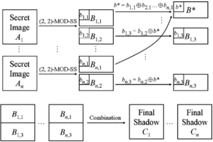
Sharing phase. 关See 共2, 2兲-MOD-SS in left-top part of

Fig.1.兴

Step 1. Use a prime number key to generate a permuta-tion sequence to permute all pixel posipermuta-tions of the given grayscale image A. Then attach the key in the permuted image A˜ .

Step 2. Sequentially read in gray values 兵pi其 of A˜, and

then store in array E according to the rules. Step 2.1. If pi⬍250, then store piin E.

Step 2.2. If pi⭌250, then split pi into two values 250

and 共pi− 250兲. Store these two values in E 共first 250,

then pi− 250兲.

Step 3. Sequentially grab two not-shared-yet elements a₀ and a1 of E. Use the grabbed共a0, a1兲 to evaluate

b1= q共1兲 = 共a0+ a1兲Mod 251, 共2兲

b₂= q共2兲 = 共a₀+ a₁⫻ 2兲_{Mod 251}, 共3兲 and then attach b₁ to shadow B₁, and attach b₂ to shadow B2.

Step 4. Repeat step 3 until all elements of the array E are processed.

Notably, step 2.2 handles the gray values larger than 250 共see Ref.14兲, which seldom happens for most natural im-ages. Therefore, the size of E, which equals the total size of

B1 and B2, is very close to size A. In other words, each created B1and B2is about two times smaller than A in size.

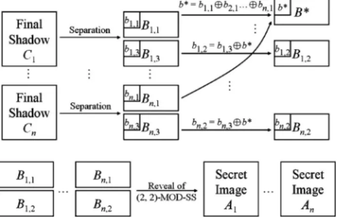
Reveal phase. 关See Reveal of 共2, 2兲-MOD-SS in the

bot-tom part of Fig.2.兴

Step 1. Take the first nonused pixel from each of the two shadows B1and B2. Call the two values共b1, b2兲.

Step 2. Use these two values共b1, b2兲 to recover the two coefficients共a0, a1兲 in Eqs.共2兲 and共3兲 by

a₁=共b2− b₁+ 251兲Mod 251, 共4兲

a0=共b1− a1+ 251兲Mod 251. 共5兲

The recovered共a0, a1兲 are the two corresponding values in E.

Step 3. Repeat steps 1 and 2 until all values of the two shadows B₁and B₂ are processed.

Step 4. Sequentially grab an element pi of E, then do:

Step 4.1. If pi⬍250, then store pi in A˜ . Now, delete pi

from E, because the information contained in pi has

been used.

Step 4.2. If pi= 250, then read in pi+1 immediately. Then

store the single value共250+pi+1兲 in A˜. Now, delete both pi and pi+1 from E, because the information in pi and pi+1have both been used.

Step 5. Extract the prime number key from A˜ and apply the inverse-permutation operation to the permuted image

A

˜ to get back to the secret image A.

In this reveal algorithm, only three operations 共one SUB, one ADD, and one MOD兲 are needed in Eqs. 共4兲or 共5兲to reconstruct each secret pixel of A˜ . Because usually there are only a few pixels in A 共and hence in A˜兲 whose gray values are above 250, the ADD operation in step 4.2 sel-dom occurs. Also, for each pixel, step 5 uses one mapping operation共indexing兲 rather than computational operation. 2.2 Exclusive-OR-Based共n,n兲 Shadows

Combination Tool

Once all given n secret images A1, A2, . . . , Anare processed

by the MOD-based共2, 2兲 secret sharing tool described in Sec. 2.1, each secret image Ai 共1艋i艋n兲 generates two

half-size temporary shadows Bi,1 and Bi,2. To avoid any

secret leaking when collecting less than n final shadows, we use the following steps of a combination phase to form the final shadow Ci.

Combination phase. 共See right-top and bottom parts of

Fig.1.兲

Step 1. Size-synchronization: if some shadows B_i,j 共1 艋i艋n and 1艋 j艋2兲 have distinct size due to the exis-tence of pixels whose gray values are in 251 to 255 in some images Ai, then add a suitable number of dummy

pixels in all shadows to make all shadows Bi,jhave the

same size as the one with the largest size.

Step 2. Stacking: take the first not-yet-processed pixel

bi,1from each shadow Bi,1共1艋i艋n兲. Then evaluate the

corresponding pixel b*for a new image B*by

b*= b_1,1丣b_2,1丣 ¯ 丣b_n,1. 共6兲 After all pixels of all Bi,1 are processed, the generation

of image B*is done, and its size is the same as Bi,1共and Bi,2, too兲.

Step 3. Shifting B_i,2to B_i,3: take next not-yet-processed pixel bi,2 from each shadow Bi,2 共1艋i艋n兲, and at the

same pixel position take the corresponding pixel b* 苸B*. Then create the corresponding pixel value bi,3of a

new image Bi,3by

bi,3= bi,2丣b* 共1 艋 i 艋 n兲. 共7兲

After all pixels in all Bi,2are processed, all n images Bi,3

are generated. Notably, each Bi,3is as large as each Bi,2.

Step 4. Physically gluing: for 1艋i艋n, physically com-bine each pair of Bi,1 and Bi,3 to generate their final

shadow Ci=共Bi,1; Bi,3兲. Because Bi,1 and Bi,3 are both

about two times smaller than Ai, each Ci is about as

large as Ai.

When all n final shadows C1, C2, . . . , Cn are gathered,

we can reconstruct all Bi,1and Bi,2共1艋i艋n兲 by using the

following steps of a decomposing phase whose computa-tion is very low.

Decomposition phase. 关See top part of Fig.2.兴

Step 1. For 1艋i艋n, physically separate each Ci

=共Bi,1; Bi,3兲 into two halves to get Bi,1 共front half兲 and Bi,3 共rear half兲.

Step 2. Take next not-yet-processed pixel bi,1from each B_i,1共1艋i艋n兲. Then evaluate the corresponding pixel b* in the image B*by Eq.共6兲. After all pixels of all B_i,1are processed, the image B*is generated.

Step 3. Take next not-yet-processed pixel bi,3from each Bi,3 共1艋i艋n兲, and at the same pixel position, take the

corresponding pixel b*from B*. Then evaluate the cor-responding pixel bi,2for each image Bi,2 by

bi,2= bi,3丣b* 共1 艋 i 艋 n兲. 共8兲

After all pixels of all B_i,3 are processed, all B_i,2 are recovered.

On average, only one XOR operation is needed to re-cover a pixel of a secret image, and this statement is true for each secret image Ai共1艋i艋n兲. The analysis is as

lows. Assume size of each Aiis w⫻h, then each Bi,1in step

2 uses on average关共n−1兲/n兴⫻关共w⫻h兲/2兴 XOR operations in Eq. 共6兲 to create B*. And each Bi,3 in step 3 uses on

average 共w⫻h兲/2 XOR operations in Eq. 共8兲 to recover

Bi,2. Therefore, for each secret image Ai, the total number

of XOR operations needed in the decomposition phase is 兵关共n−1兲/n兴+1其⫻关共w⫻h兲/2兴, which will be smaller than 1 after dividing by Ai’s size w⫻h. In other words, less than

one XOR operation is needed in the decomposition phase to recover a pixel of a secret image Ai.

3 Proposed Method

3.1 Encoding

The encoding uses the sharing phase of the MOD-based共2, 2兲 secret sharing tool in Sec. 2.1, followed by the combi-nation phase of the XOR-based共n,n兲 shadows combination tool in Sec. 2.2. The encoding creates n shadows

C1, C2, . . . , Cn to replace the n given secret images A₁, A₂, . . . , An. The main steps are as follows.

Encoding algorithm. 共The diagram is in Fig.1.兲

Input: n input binary/grayscale/color secret images

A1, A2, . . . , Anof the same size.

Step 1. It does not matter whether the image is binary or gray or color, just treat each Ai 共1艋i艋n兲 as a long

byte-stream共so each element has 8 bits and can be con-sidered as a gray-value pixel兲.

Step 2. Then, for each stream Ai共1艋i艋n兲, use the

shar-ing phase of MOD-based 共2, 2兲 secret sharing tool in Sec. 2.1 to create its half-size shadows兵B_i,1, B_i,2其. Step 3. Use all 兵B_i,1, B_i,2其 1艋i艋n in the combination phase of the XOR-based 共n,n兲 shadows combination tool in Sec. 2.2 to generate n final shadows

C1, C2, . . . , Cn.

Notably, each final shadow Ciis共nearly兲 as large as Ai.

As a result, even from a multisecrets view, the I/O size ratio is also 1, because total secret size兩兵A1, A2, . . . , An其兩 is

iden-tical to the total shadow size兩兵C1, C2, . . . , Cn其兩.

3.2 Decoding

To recover the n secret images A1, A2, . . . , An from the n

final shadows C₁, C₂, . . . , Cn, the decoding uses the

decom-position phase of the XOR-based共n,n兲 shadows combina-tion tool in Sec. 2.2, followed by the reveal phase of the MOD-based共2, 2兲 secret sharing tool in Sec. 2.1. The main steps are as follows.

Decoding algorithm. 共See the diagram in Fig.2.兲 Step 1. Use the decomposition phase of the XOR-based 共n,n兲 shadows combination tool in Sec. 2.2 to recon-struct the half-size images兵Bi,1; Bi,2其1艋i艋n from the n

final shadows兵C1, C2, . . . , Cn其.

Step 2. For each pair兵Bi,1; Bi,2其, where 1艋i艋n, use the

reveal phase of the MOD-based共2, 2兲 secret sharing tool in Sec. 2.1 to recover the secret image Ai from

兵Bi,1; Bi,2其.

Step 3. If the original secret images are not gray-valued, then transform all n 8-bit images A1, A2, . . . , An to their

binary/color equivalent.

On average, the decoding only needs one XOR, one MOD, one ADD, and one SUB operations共all are between bytes兲 to reconstruct each 1-byte 共8-bit兲 pixel value of a secret image. 共In step 1 of decoding, one XOR operation is needed to recover a 1-byte pixel value of Bi,2 for the

de-composition phase of the XOR-based共n,n兲 shadows com-bination tool. In step 2, one MOD, one ADD, and one SUB operations are needed to recover a 1-byte pixel value of Ai

in the reveal phase of the MOD-based共2, 2兲 secret sharing tool.兲

4 Experimental Result and Comparisons

4.1 Experimental Result

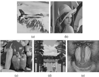
In the experiment here, without the loss of generality, let

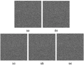
n = 5 and let the n input images 兵A1, A2, . . . , A5其 be the 512⫻512 grayscale images 兵Jet, Lena, Pepper, Scene, and Monkey其 shown in Figs. 3共a兲–3共e兲. Then, Figs. 4共a兲–4共e兲 show the n = 5 final shadows 兵C1, C2, . . . , C5其 generated in Sec. 3.1, and each 512⫻512 shadow is as large as each input image. Figures5共a兲–5共e兲show five error-free recov-ered images A1, A2, . . . , A5 共Jet, Lena, Pepper, Scene, and Monkey兲 in Sec. 3.2 using all n=5 final shadows

C1, C2, . . . , C5. In general, all recovered images in our method are error-free, i.e., the peak signal-to-noise ratio 共PSNR兲 value is infinity 共⬁兲 for each of our recovered im-ages. So each of the recovered images兵Jet, Lena, Peppers, Scene, and Monkey其 shown in Fig. 5 has PSNR=⬁. 共The five images in Fig. 5 and the five images in Fig. 3 are exactly the same, rather than just similar.兲

In addition, to show our constant decoding-time prop-erty in the retrieval, we also listed in Table1the number of operations on average needed to decode each one of the n secret images. It can be seen that, indeed, a constant num-ber of operations is needed for each value of n. The actual CPU time taken in decoding is also checked in a computer. We still find that our decoding time does not vary as the value of n varies.

4.2 Comparisons

Table 2 compares our method with other multisecret schemes7–10 in terms of two quantifiable measures: 1. I/O size ratio and 2. decoding computational complexity. For comparison, the same conditions hold for each scheme. They are: 1. there are n secret images, 2. every recovered image must be lossless, and 3. the computer versions of VC schemes8,9 are implemented using an OR-like operation to simulate the stacking action of transparencies. From Table 2, we can see that our method not only keeps the I/O size ratio as large as 1, but also needs only constant decoding operations to reconstruct a secret pixel. Other schemes7–10 either have I/O size ratio smaller than 1, or need noncon-stant decoding complexity to reconstruct a secret pixel. For completeness, we also include in Table 2 the very fast methods11–13 developed by Muñoz-Rodríguez and Rodríguez-Vera that use one secret image and one pattern

image as input. Their I/O size ratios are as good as ours. Their decoding complexity is very economic, but their de-coding only gives approximated versions共rather than error-free recovery兲 of the original image. So theirs and ours have different highlighting.

Fig. 4 The five generated noisy shadows_兵C1, C₂, . . . , C_{5其 in the n} = 5 case. Their PSNRs are all around 8.0 if we compare them with the secret image Jet共all around 9.5 if we compare them with Lena; all around 9.2 if we compare them with Peppers; all around 8.6 if we compare them with Scene; all around 9.7 if we compare them with Monkey兲.

Fig. 5 The five error-free images共PSNR=⬁兲 recovered by using all five shadows共Fig.4兲 in the n=5 case.

Table 1 Number of operations needed to decode each one of the n secret images whose sizes are all 512⫻512.

Value of n

Number of operations needed to de-code one 512⫻512 secret image

2 512⫻512 XOR, 512⫻512 MOD, 512

⫻512 ADD, 512⫻512 SUB operations

3 512⫻512 XOR, 512⫻512 MOD, 512

⫻512 ADD, 512⫻512 SUB operations

4 512⫻512 XOR, 512⫻512 MOD, 512

⫻512 ADD, 512⫻512 SUB operations

5 512_{⫻512 XOR, 512⫻512 MOD, 512}

⫻512 ADD, 512⫻512 SUB operations

6 512⫻512 XOR, 512⫻512 MOD, 512

⫻512 ADD, 512⫻512 SUB operations

7 512_{⫻512 XOR, 512⫻512 MOD, 512}

⫻512 ADD, 512⫻512 SUB operations

8 512⫻512 XOR, 512⫻512 MOD, 512

⫻512 ADD, 512⫻512 SUB operations

9 512⫻512 XOR, 512⫻512 MOD, 512

⫻512 ADD, 512⫻512 SUB operations

… 512⫻512 XOR, 512⫻512 MOD, 512

⫻512 ADD, 512⫻512 SUB operations

Table 2 I/O size ratio and decoding complexity. For I/O size ratio, total size of input images is divided by total size of shadows. Hence, larger is better. For decoding complexity, complexity is to decode a pixel of a secret image. For math operators, k is a user-specified threshold value, e.g., k = 0.5n or k = 2. For Ref.10, math operations: ⫹, ⫺, ⫻, ⫼. References11–13are very fast, but the decoding just gives approximated versions_{共rather than an error-free version兲 of} the original secret image.

Schemes

I/O size ratio

共larger is better兲 Decoding complexity共smaller is better兲

Ref.7 1 / 2⬃1 O共log2_{k兲 共math operations兲}

Ref.8 1 / 4 2⫻n 共OR-like operations兲

Ref.9 1 / 6 3_{⫻n 共OR-like operations兲}

Ref.10 n /共n+1兲 1共MOD operation兲 and

O共n兲 共math operations兲

Refs.11–13 1 1 overlapping operation

Our scheme 1 1 XOR, 1 MOD, 1 ADD,

5 Security Analysis

In this section, we analyze the security of the encrypted images共shadows兲.

5.1 Probability

Assume that only n − 1 final shadows are available, and a shadow Cjis missing. Then, people cannot obtain B*

cre-ated by b*= b1,1丣b2,1丣¯丣bn,1in Eq.共6兲, due to the lack

of the b_j,1, which is in the front half of Cj. Wthout B*,

people cannot reconstruct B1,2, B2,2, . . . , Bn,2 defined by bi,2= bi,3丣b* 共1艋i艋n兲 in Eq. 共8兲. As a result, no secret

image Ai can be recovered 关see the reveal phase of the

MOD-based 共2, 2兲 secret sharing tool in Sec. 2.1兴 due to absence of all Bi,2共1艋i艋n兲.

Next we discuss the probability of obtaining some right secret images Aithrough guessing. Without the loss of

gen-erality, assume that a betrayal party of n − 1 participants gathers their n − 1 final shadows C1, C2, . . . , Cn−1, and try to

recover some of the n secret images without the coopera-tion of the missing shadow Cn. From Eqs.共6兲and共8兲, we

have

bi,2= bi,3丣b*= bi,3丣b1,1丣b2,1丣 ¯ 丣bn,1

共1 艋 i 艋 n兲. 共9兲

Because of the lack of Cn=关Bn,1; Bn,3兴, for each pixel bn,1in Bn,1, the betrayal party will have to guess a value, and then

they use this guessing value to get a set of n − 1 pixel values

b1,2, b2,2, . . . , bn−1,2 in B1,2, B2,2, . . . , Bn−1,2, respectively, at

the same pixel position共there is no bn,2value in Bn,2due to

lack of bn,3兲. Then, the 2⫻共n−1兲 secret pixels in A₁, A₂, . . . , A_n−1can be reconstructed by using b_i,1 and b_i,2 共1艋i艋n−1兲 in the reveal phase of the MOD-based 共2, 2兲 secret sharing tool in Sec. 2.1. This is just to reconstruct two pixels in each Ai共1艋i艋n−1兲. This value guessing of

one pixel, like bn,1, will repeat共w⫻h兲/2 times if the size of

each Aiis w⫻h 共then, the size of Bn,1is 0.5⫻w⫻h兲.

From this description, we can evaluate the probability of obtaining some right grayscale images Ai of size w⫻h as

follows: probability =

冉

冊

冉

冊

Bn,1. In fact, for each secret image Ai 共1艋i艋n兲 in the

encoding process关as we did in step 1 of the sharing phase of the MOD-based共2, 2兲 secret sharing tool in Sec. 2.1兴, we already use a prime number as a key共a seed兲 of a random number generator to rearrange all the pixel positions of Ai.

Even if many pixel values in Bn,1are guessed successfully,

in step 4 of the reveal phase of the MOD-based共2, 2兲 secret sharing tool in Sec. 2.1, the recovered images A˜i 共1艋i

艋n−1兲 are still extremely noisy. Therefore, the security guardian has double levels.

For instance, in the experimental example of Sec. 4.1, if we only get four shadows, say C1, C2, . . . , C4 in Figs. 4共a兲–4共d兲, and then guess the pixel values of images B_5,1

Table 3 The entropy and PSNR values of the five generated noisy shadows_兵C1, C₂, . . . , C_{5其 shown in} Fig.4.

The five shadows C1 C2 C3 C4 C5

Entropy values 7.999 7.999 7.999 7.999 7.999 PSNR values共Jet兲 8.059 8.055 8.047 8.056 8.036 PSNR values共Lena兲 9.473 9.514 9.506 9.501 9.495 PSNR values共Peppers兲 9.202 9.204 9.206 9.186 9.213 PSNR values_共Scene兲 8.594 8.601 8.603 8.571 8.593 PSNR values共Monkey兲 9.703 9.704 9.698 9.705 9.699

Fig. 6 The n = 5 images A1, A2, A3, A4, A5recovered by using only four shadows C1, C2, C3, C4关Figs.4共a兲–4共d兲兴 and two guessed im-ages B_5,1and B_5,2in the n = 5 case.

and B5,2, then the five recovered images of A1, A2, . . . , A5 are the extremely noisy images shown in Fig.6.

5.2 Dissimilarity between Shadow Images

In the case of sensitivity, the difference between two shadow images cannot be observed visually. For this mat-ter, we check the dissimilarity between shadow images as

follows. First, from Table3, we can see that all generated shadows have very similar entropy共7.999兲 and very similar PSNRs 共when they are all compared with a secret image, say Lena兲. Second, besides comparing a shadow 共Ci兲 with a

secret image, if a shadow Ci is compared with another

shadow Ci共1艋i⬍ j艋5兲, then a PSNR value called

PSNR共Ci, Cj兲 can be evaluated by the formula

PSNR共Ci,Cj兲 = 10 ⫻ log10

2552

兺u=1512兺v=1512关Ci共u,v兲 − Cj共u,v兲兴2/共512 ⫻ 512兲

, 共10兲

and the computation result is as listed in Table4. From this table, we can see that the PSNR共Ci, Cj兲 values are all very

low共smaller than 9兲 for all pairs of shadows 共Ci, Cj兲. This

means that none of the shadows are alike. Third, none of the shadow Ciin兵C1, . . . , C5其 can be predicted in any part

from another shadow Ci, because each difference image

兩Ci− Ci兩 共see Fig. 7兲 between two shadows Ci and Cj 共1

艋i⬍ j艋5兲 still looks extremely noisy and has neither a meaningful pattern nor meaningful contour. From the end of Fig. 7, we also see that the ten histograms for 兩Ci

− Cj兩1艋i⬍j艋5 all look alike 共due to space limitation, only

two of the ten are shown兲, and this fact implies that the ten entropies for the ten difference images兵兩Ci− Cj兩其1艋i⬍j艋5are

almost identical共the entropy of each difference image reads 7.673…, as shown in Table4.兲 From Fig.7and Table4, no shadow can be predicted in any part from another shadow.

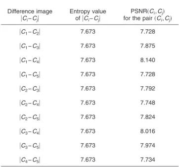
Table 4 The entropy of the difference image _兩Ci− C_{j兩, and the} PSNR共Ci, Cj兲 value. 共The two shadow images Ciand Cjare taken

from the five shadow images兵C1, . . . , C5其 shown in Fig.4. So there are 5! ÷关2!共5−2兲!兴=10 pairs.兲 Difference image 兩Ci− Cj兩 Entropy value of_兩Ci− C_j兩 PSNR_共Ci, C_j兲 for the pair_共Ci, C_j兲

兩C1− C2兩 7.673 7.728 兩C1− C3兩 7.673 7.875 兩C1− C4兩 7.673 8.140 兩C1− C5兩 7.673 7.728 兩C2− C3兩 7.673 7.792 兩C2− C4兩 7.673 7.748 兩C2− C5兩 7.673 7.824 兩C3− C4兩 7.673 8.016 兩C3− C5兩 7.673 7.974 兩C4− C5兩 7.673 7.734

Fig. 7 The ten difference images 兵兩C1兩−兩C2兩,兩C1兩−兩C3兩,兩C1兩 −兩C4兩,兩C1兩−兩C5兩,兩C2兩−兩C3兩,兩C2兩−兩C4兩,兩C2兩−兩C5兩,兩C3兩−兩C4兩,兩C3兩 −兩C5兩,兩C4兩−兩C5兩其; and the two histograms for 兩C1− C2兩 and 兩C1− C3兩, respectively. The remaining 10− 2 = 8 histograms all look like these two histograms, so their entropies all read 7.673…, as shown in Table4.

5.3 Statistical Analysis

Many attackers use statistical analysis to analyze the en-crypted images to trace back the original secret images. So we also apply statistical analysis to our shadows. It includes the following: the histogram of each shadow is inspected in Sec. 5.3.1; the correlations of two adjacent pixels of each shadow are examined in Sec. 5.3.2; and the number of pix-els change rate 共NPCR兲 and unified average changing in-tensity共UACI兲 values are examined in Sec. 5.3.3 to check the relationship between the original images 共secrets兲 and the encrypted images共shadows兲.

5.3.1 Histograms, entropies, and peak signal-to-noise ratios of the encrypted images

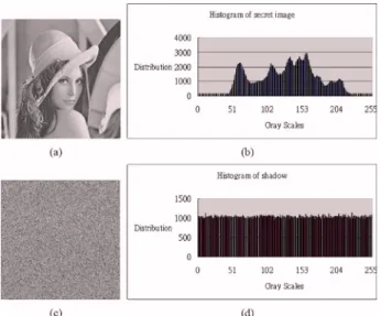
We still inspect the five images in Fig. 3 whose image contents are of quite different styles共airplane, human face, vegetable, scenery, and animal兲. The histograms of the five input images and the histograms of the five created shad-ows are compared. A typical example of the comparison is shown in Fig. 8. The histogram of each encrypted image 共shadow兲 is fairly uniform, and it is significantly different from the histogram of any input secret image共e.g., Lena兲. The same observation also exists for the shadows created using other sets of n secret images.

In general, besides the histogram, entropy is another useful value to measure the information distribution of an image. If an image has G gray levels 共G艋256兲, and the probability of gray-level k共0艋k艋G−1兲 is P共k兲, then the image’s entropy Heis

He= −

兺

k=0 G−1

P共k兲log2关P共k兲兴. 共11兲

The entropy value of the secret image Lena in Fig.8共a兲is

He共Lena兲=7.327, and the entropy value of the shadow

im-age in Fig. 8共c兲 is He共shadow image兲=7.999. Note that

7.999 is very close to the perfect entropy value

8 = −

兺

冉

冊

冉

冊

which is the entropy value for an ideal image whose gray values are of exactly uniform distribution. He共shadow

im-age兲 is almost 8, because the gray values of each shadow are almost uniformly distributed. In view of security, shadow images with entropy values very close to 8 are good, because it means that the original secret information is now widely and uniformly spread over the shadow im-ages. We have also checked the entropy values of the shad-ows created from other sets of secret images; and the en-tropy values of the shadows are still very close to 8.

In terms of PSNR, we include in Table 3 the PSNR values of the five generated shadow images printed in Fig. 4. As shown in Table3, if we randomly pick a shadow Ci

共i=1, 2, 3, 4, 5, because n=5兲 in Fig.4, and compare this randomly chosen shadow with the secret image Jet in Fig. 3, then the PSNR value is in a very concentrated range 共between 8.036 and 8.059, as shown in row 3 of Table3兲. Likewise, if we compare the randomly chosen shadow with the secret image Lena, then the PSNR value is still in a very concentrated range 共between 9.473 and 9.514, as shown in row 4 of Table 3兲. Similar observation exists in the remaining rows of Table3, if the secret image is being compared with Peppers 共or Scene or Monkey兲. The phe-nomenon that shadows 兵C1, . . . , C5其 are so alike in both entropy and PSNRs indicates that the shadows are very similar in pixel distribution. Also note that the PSNR values appeared in Table3are all very low共less than 10兲, and this indicates that each of these extremely noisy shadows 兵C1, . . . , C5其 in Fig.4 looks completely different from any of the five original secret images shown in Fig.3. Thus, the hackers can hardly guess what the original secret images are.

5.3.2 Correlation of two adjacent pixels

In the subsection, we examine the correlation between two 共vertically/horizontally/diagonally兲 adjacent pixels. As quoted from Ref.15, for a given image, its correlation co-efficient between adjacent pixels is computed according to the formula

rxy=

_冑

D共x兲

冑

Here, the symbol 共x,y兲 represents the random variable of the gray values of two adjacent pixels. Notably, for an im-age, if there are N pairs of共x,y兲, then we compute

E共x兲 = 1 N

兺

兺

兺

兺

Fig. 8 Histograms of the original and encrypted images._{共a兲 is one} of the n = 5 input secret images;共b兲 is the histogram of 共a兲; 共c兲 is a typical shadow image; and共d兲 is the histogram of 共c兲.

cov共x,y兲 = 1

N

兺

关xi− E共x兲兴关yi− E共y兲兴, 共15兲

to get rxy. Figure 9共a兲shows the distribution of two

adja-cent pixels 共x,y兲 for the secret image Lena in Fig. 8共a兲. Then, Fig.9共b兲 shows the distribution for the shadow im-age sketched in Fig. 8共c兲. The correlation coefficients are 0.360456 and 0.004678, respectively. In general, the corre-lation coefficient is high for each secret image, and very low for each shadow.

5.3.3 Differential analysis

Here, the number of pixels change rate共NPCR兲 and unified average changing intensity共UACI兲 are checked. In general, when a pixel value is changed in one of the n secret images, two measures NPCR and UACI can be utilized to describe the impact to the n shadow images. Details are as follows.

Assume that we change a pixel value in one of the n input secret images—for example, change a pixel value for the Lena image shown in Fig. 3共b兲. Before this one-pixel change, let the n corresponding shadow images be 兵C1, . . . , Cn其. Then, after this one-pixel change of the secret

image Lena, let the n generated shadow images be 兵C1

⬘

⬘

⬘

shadow, let Ck共i, j兲 and Ck

⬘

val-ues at position共i, j兲, respectively. The NPCRkfor shadow k

is defined as

NPCRk=

兺i,jDk共i, j兲

W⫻ H ⫻ 100%, 共16兲

where W and H are the width and height of a shadow. In the evaluation of NPCRkfor shadow k, the comparison record Dk is defined as the binary matrix in which Dk共i, j兲=0 if Ck共i, j兲=Ck

⬘

⬘

Nota-bly, NPCRk measures the percentage of the altered pixels

for shadow k 共0% means the two versions Ck and Ck

⬘

shadow k are identical everywhere兲. The UACIkfor shadow k is defined as

UACIk=

1

W⫻ H

冋

兺

兩Ck共i, j兲 − Ck

⬘

255

册

which measures the average intensity of the differences be-tween the two versions共Ckand Ck

⬘

One of the performed tests is when the one-pixel change is on the Lena image of Fig. 3共b兲. Then the range of 兵NPCR1, . . . , NPCRn其 for the n shadows is from 99.60 to

99.63%, and the range of兵UACI1, . . . , UACIn其 for n

shad-ows is from 33.20 to 33.40%. The average of

兵NPCR1, . . . , NPCRn其 is NPCRaverage= 99.6111%, and the

average of兵UACI1, . . . , UACIn其 is UACIaverage= 32.2980%.

When the one-pixel change is on any other image of Fig.3, the average value of 兵NPCR1, . . . , NPCRn其 is still larger

than 99.6%; and the average value of兵UACI1, . . . , UACIn其

is still larger than 33.2%. Therefore, a one-pixel change in any secret image can cause a significant change to all n shadow images. Hence, our shadows can resist differential attack in which the opponents, as mentioned in Refs. 15 and16, make a slight change in the secret image, and then observe the result in the shadow images. In this way, the opponents try to find a meaningful relationship between the pixels of the secret image and the pixels of the shadows. In our system, since one minor change in the secret image can cause a significant change in all shadows, the differential attack would become useless.

6 Summary and Future Works

A novel lossless sharing scheme for multiple secret images is designed using MOD and XOR operations. Our advan-tages are: 1. the total size of n given secret images is the same as the total size of the n final shadows共hence our I/O size ratio is 1兲; 2. we only need one XOR, one MOD, one ADD, and one SUB共all are byte-to-byte兲 operations to get a lossless recovery of each secret pixel’s 8-bit value for the

Fig. 9 Distribution of the pairs of adjacent pixels._{共a兲 is for the secret} image Lena sketched in Fig.8共a兲, whereas共b兲 is for the shadow image sketched in Fig.8_共c兲.

given binary/grayscale/color images共so our decoding com-putational complexity for each pixel is a constant and inde-pendent of n兲.

Our method is better than other lossless multisecret schemes in terms of two quantity measures: I/O size ratio and decoding time. But Ref. 7–10 have features of their own. 1. Feng et al.’s7uses generalized access structures to achieve higher flexibility, and each qualified set of the ac-cess structure is able to share secret images independently. 2. If the shadows are printed in transparencies, then the VC schemes8,9can also reveal images by doing physical stack-ing of transparencies although true-color images will be very hard for VC to retrieve error-free by stacking transpar-encies. 3. Alvarez et al.’s method10 can process n given secret images of nonequal sizes. To improve our multisecret sharing scheme in the future, the advantages of these others will be our main guidelines.

Acknowledgments

This work is supported by National Science Council, Tai-wan, under grant NSC 97-2221-E-009-120-MY3. The au-thors also thank the reviewers for valuable suggestions.

References

1. A. Shamir, “How to share a secret,”Commun. ACM22共11兲, 612–613 共1979兲.

2. M. Naor and A. Shamir, “Visual cryptography,” in Adv. Cryptolog. EUROCRYPT’94, 950, 1–12共1995兲.

3. R. Z. Wang and C. H. Su, “Secret image sharing with smaller shadow images,”Pattern Recogn. Lett.27, 551–555共2006兲.

4. C. C. Lin and W. H. Tsai, “Visual cryptography for gray-level images by dithering techniques,”Pattern Recogn. Lett.24, 349–358共2003兲. 5. Y. C. Hou, “Visual cryptography for color images,”Pattern Recogn.

36, 1619–1629共2003兲.

6. S. J. Lin and J. C. Lin, “VCPSS: A two-in-one two-decoding-options image sharing method combining visual cryptography 共VC兲 and polynomial-style sharing 共PSS兲 approaches,” Pattern Recogn. 40, 3652–3666共2007兲.

7. J. B. Feng, H. C. Wu, C. S. Tsai, and Y. P. Chu, “A new multi-secret images sharing scheme using Largrange’s interpolation,” J. Syst. Softw.76, 327–339共2005兲.

8. S. J. Shyu, S. Y. Huang, Y. K. Lee, R. Z. Wang, and K. Chen, “Shar-ing multiple secrets in visual cryptography,”Pattern Recogn. 40, 3633–3651共2007兲.

9. J. B. Feng, H. C. Wu, C. S. Tsai, Y. F. Chang, and Y. P. Chu, “Visual secret sharing for multiple secrets,”Pattern Recogn.41, 3572–3581 共2008兲.

10. G. Alvarez, L. H. Encinas, and A. M. del Rey, “A multisecret sharing scheme for color images based on cellular automata,” Inf. Sci. 178, 4382–4395共2008兲.

11. J. A. Muñoz-Rodríguez and R. Rodríguez-Vera, “Image encryption based on moiré pattern performed by computational algorithms,”Opt. Commun.236共4–6兲, 295–301 共2004兲.

12. J. A. Muñoz-Rodríguez and R. Rodríguez-Vera, “Image encryption based on a grating generated by a reflection intensity map,”J. Mod. Opt.52共10兲, 1385–1395 共2005兲.

13. J. A. Muñoz-Rodríguez and R. Rodríguez-Vera, “Image encryption based on phase encoding by means of a fringe pattern and computa-tional algorithms,” Revista Mexicana de Física 52共1兲, 53–63 共2006兲. 14. C.-C. Thien and J.-C. Lin, “Secret image sharing,”Computers and

Graphics26共5兲, 765–770 共2002兲.

15. H. El-din, H. Ahmed, H. M. Kalash, and O. S. Farag Allah, “Encryp-tion efficiency analysis and security evalua“Encryp-tion of RC6 block cipher for digital images,” Intl. J. Computer, Info. Syst. Sci. Eng. 1共1兲, 33–39 共2007兲.

16. G. Chen, Y. B. Mao, and C. K. Chui, “A symmetric image encryption scheme based on 3D chaotic cat maps,”Chaos, Solitons Fractals

21共3兲, 749–761 共2004兲.

Kun-Yuan Chao received his BS degree in computer and information science in 1996 from National Chiao Tung University, Tai-wan. Then he received his MS degree in computer science and information engineer-ing in 1999 from National Taiwan University, Taiwan. He is currently a PhD candidate in the Department of Computer and Informa-tion Science, NaInforma-tional Chiao Tung Univer-sity, Taiwan. His recent research interests include secret image sharing, visual cryp-tography, and image processing.

Ja-Chen Lin received his BS degree in computer science and MS degree in applied mathematics, both from National Chiao Tung University, Taiwan. He received his PhD degree in mathematics from Purdue University, Lafayette, Indiana. He joined the Department of Computer and Information Science at National Chiao Tung University in 1988, and then became a professor there. His research interests include pattern recognition and image processing.