利用數位相機建構三維物體點結構

國 立 交 通 大 學

資訊科學與工程研究所

碩 士 論 文

利用數位相機建構三維物體點結構

3D Object Point Structure Construction Using a Digital

Camera

研 究 生：吳昶澔

指導教授：陳稔 教授

利 用 數 位 相 機 建 構 三 維 物 體 點 結 構

3D Object Point Structure Construction Using a Digital Camera

研 究 生：吳昶澔 Student：Chang-Hao Wu

指導教授：陳稔

Advisor：Zen Chen

國 立 交 通 大 學

資 訊 科 學 與 工 程 研 究 所

碩 士 論 文

A Thesis

Submitted to Institute of Computer Science and Engineering College of Computer Science

National Chiao Tung University in partial Fulfillment of the Requirements

for the Degree of Master

in

Computer Science June 2006

Hsinchu, Taiwan, Republic of China

利 用 數 位 相 機 建 構 三 維 物 體 點 結 構

研 究 生：吳昶澔

指導教授：陳稔

國 立 交 通 大 學

資 訊 科 學 與 工 程 研 究 所

摘要 本論文的目的在於利用相機與物體的相對運動做連續拍攝來重建出物體的 三維點結構與各個視角的投影矩陣。三維點結構本身可以使用在辨識與提供物體 的幾何資訊，而各視角中的投影矩陣配合物體投影的輪廓資訊可以做物體密集的 幾何重建(dense reconstruction)。 文獻中對於由影像序列恢復結構與運動的方法大都要求完美的影像特徵點 對應，也就是所追蹤的特徵點在所有的圖片中都不能遺失，而且所追蹤的特徵點 位置沒有雜訊，然而完美的特徵點對應需求會嚴重限制實際的應用性。本論文使 用了 multi-view reconstruction method 和 iterative reweighted least square(IRLS)來 做強健式的透視投影空間(projective space)中的結構與運動的重建，並利用 iterative absolute dual quadric 做 auto calibration 來將結果校正至歐式幾何空間。 本論文把此系統應用在人頭的辨識與密集重建上，初步證實了本論文所提出的系 統藍圖是具有實際應用性的價值。

3D Object Point Structure Construction with a Digital Camera

Student：Chang-Hao

Wu Advisor：Zen Chen

Institute of Computer Science and Engineering College of Computer

Science

National Chiao Tung University

Abstract

The current algorithms for recovering the scene structure and camera motion from an image stream require a set of well-tracked features. Such a set is in general not available in practical applications. Thus, there is a need for making the recovering structure and motion algorithm deal effectively with missing features and data noise in the tracked features.

We propose a new scheme combining the multi-view reconstruction method and the iterative reweighted least square method. This scheme is able to deal effectively with the missing features and noise in the individual features. Furthermore, the proposed scheme includes an auto-calibrated method for Euclidean reconstruction using the iterative absolute dual quadric framework. The robustness of the proposed scheme is tested on both the synthetic data and the real data. For the real data, the scheme is applied to the human head recognition and the dense reconstruction of human head geometry.

Acknowledgement

First of all, I would like to express my sincere appreciation to my advisor, Dr. Zen Chen, for his helpful guidance, careful supervision and encourage throughout my Master degree. Under his guidance, he shows me a way how to treat and analyze the problem.

In the past of two years, he has stimulated the research work and also offered an excellent research environment at the PAIS laboratory. I would also express my gratitude to all the members in the PAIS laboratory, for their encouragements, assistances, useful suggestions and comments. I am grateful to all of my friends for their supports and encouragements. You have made my life wonderful and cheerful.

Finally, thank my family for their understanding, supports and loves. Life is sometimes tough; however, there is nothing to defeat us with loves of family.

Contents

Chinese abstract………... i Abstract……… ii Acknowledgement……… iii Contents………... iv List of Tables………... vi

List of Figures……….. vii

Chapter 1. Introduction……… 1

1.1. Motivation………... 1

1.2. Related work………... 1

1.3. Contribution……… 3

1.4. Thesis Organization……… 3

Chapter 2. Estimation of structure and motion in projective space………. 5

2.1. Multiple view computational methods……… 5

2.1.1. Factorization………... 5

2.1.2. Bilinear method………... 6

2.2. Outliers selection by the iterative reweighted least square(IRLS) method……… 7

2.2.1. Adaptive weighting……… 8

2.2.2. Optimization with weights……… 9

Chapter 3. Euclidean Reconstruction………... 12

3.1. Auto-calibration using the iterative absolute dual quadric method 12 3.2. Acquisition of the rectifying homography……….. 13

Chapter 4. Experimental results………... 14

4.1. Synthetic data……….. 14

4.1.1. Synthetic data without noise……….. 14

4.1.2. Synthetic data with noise………... 15

4.2. Real data with the missing data……….. 20

4.2.1. Point structure reconstruction of the real object with combination……… 20

4.2.2. Point structure recognition of the human head……….. 23

4.2.3. Dense reconstruction of the human head………... 27

Chapter 5. Conclusion and future work………... 29

5.1. Conclusion……….. 29

5.2. Future work………. 29

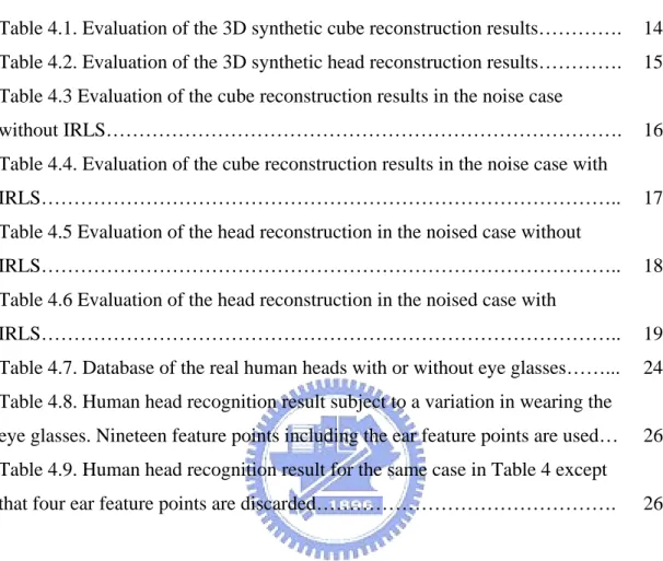
List of Tables

Table 4.1. Evaluation of the 3D synthetic cube reconstruction results…………. 14 Table 4.2. Evaluation of the 3D synthetic head reconstruction results…………. 15 Table 4.3 Evaluation of the cube reconstruction results in the noise case

without IRLS………. 16

Table 4.4. Evaluation of the cube reconstruction results in the noise case with

IRLS……….. 17

Table 4.5 Evaluation of the head reconstruction in the noised case without

IRLS……….. 18

Table 4.6 Evaluation of the head reconstruction in the noised case with

IRLS……….. 19

Table 4.7. Database of the real human heads with or without eye glasses……... 24 Table 4.8. Human head recognition result subject to a variation in wearing the eye glasses. Nineteen feature points including the ear feature points are used… 26 Table 4.9. Human head recognition result for the same case in Table 4 except that four ear feature points are discarded………. 26

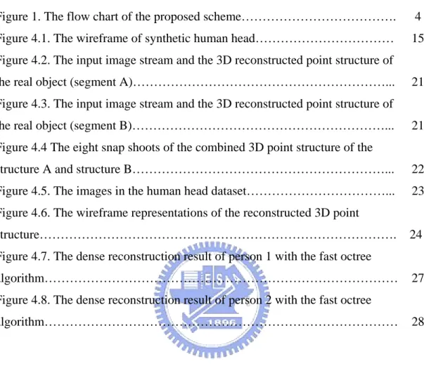
List of Figures

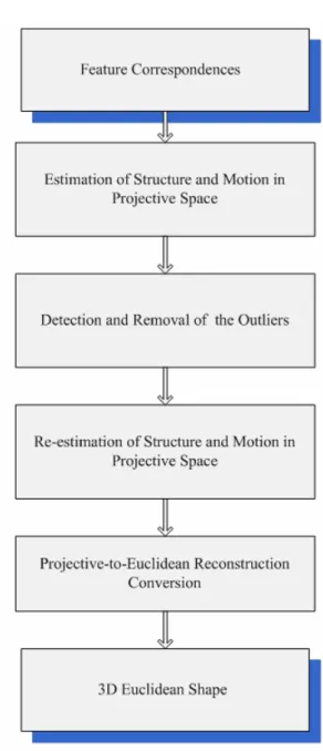
Figure 1. The flow chart of the proposed scheme………. 4 Figure 4.1. The wireframe of synthetic human head……… 15 Figure 4.2. The input image stream and the 3D reconstructed point structure of the real object (segment A)………... 21 Figure 4.3. The input image stream and the 3D reconstructed point structure of the real object (segment B)………... 21 Figure 4.4 The eight snap shoots of the combined 3D point structure of the

structure A and structure B………... 22 Figure 4.5. The images in the human head dataset………... 23 Figure 4.6. The wireframe representations of the reconstructed 3D point

structure………. 24

Figure 4.7. The dense reconstruction result of person 1 with the fast octree

algorithm……… 27

Figure 4.8. The dense reconstruction result of person 2 with the fast octree

Chapter 1. Introduction

1.1. Motivation

The inference of 3D object geometric model from multiple object images is an important problem in the computer vision community [1]-[8], leading to many applications including robotic navigation system, computer aided design, virtual reality, digital entertainment and target recognition. A common approach is to extract features from the image sequence and, then, to estimate the structure and motion of these tracked features. However, the tracked feature points generally contain noise and may not be present all the time during the image sequence. Consequently, there is a need of robust methods for applications in the real world. After the recovery of the camera models, a dense object reconstruction using the silhouettes obtained from the image sequence is made possible [1]-[2]. The dense reconstruction in the Euclidean space requires the camera calibration, which is carried out here by an auto-calibration method based on the absolute dual quadric feature [18].

1.2. Related Work

Previous approaches attempting to solve the multi-view reconstruction problem fall into several categories, depending on whether the camera is calibrated or not, and whether the camera model is perspective or affine. With a calibrated camera, one may compute Euclidean shape up to a scale factor using either an affine model or a perspective model [3], [4]. With an uncalibrated camera, the recovered shape is defined up to a projective reconstruction [5], [6]. A family of effective and popular algorithms for estimating the projective structure and motion is the so-called factorization algorithms [3] - [4], [7] - [8].

These factorization algorithms work by linearizing the camera observation model and give good results without an initial solution; hence, the factorization algorithms are a popular choice for solving the structure from motion problem. However, there is a serious drawback for factorization; that is, it requires all feature points must be visible in all views. Consider a factorization formulation with a perspective camera model [19]:

MX

D= (1)

Where D∈R3m×n is so-called data matrix.

⎟ ⎟ ⎟ ⎠ ⎞ ⎜ ⎜ ⎜ ⎝ ⎛ = mn n m m n n u z u z u z u z D 1 1 1 1 1 11 11 L M O M L (2) and

(

1

)

3 4 × ∈ = T m m R M M M _L and X

(

X Xn

)

R n × ∈ = 4

1 L are the projection matrices and the 3D points, respectively. In (2), the constant m is the total number of frames, and n is the total number of feature points. Also, u and _ij z denote the _ij

respective projected image coordinate and its perspective depth for the 3D pointX , _j

both in camera frame i. Therefore,

j i ij ij ij z u M X d = = (3)

The feature point correspondences finding is nevertheless one of the most difficult problems in the low-level image processing stage. No perfect and truly general solution has yet been presented. In most of cases, the correspondence solution relies on the situation of the application, and it cannot avoid missing some feature points in some views because of occlusion.

Moreover, it is common for bad tracked feature locations to disturb the estimation of structure and motion considerably. Previous attempts have been made at addressing this problem. Irani and Anandan [17] assume that the uncertainty is divided into the 3D feature points and the projection matrices. In other words, if a 3D feature point has a relatively high uncertainty in one frame, then it is assumed that it has a similar high uncertainty in all other frames. However, large difference in the variance of individual 2d feature points is critical to the implementation of the robust statistical techniques that can deal with the missing data and noise problems. The robust factorization [9] proposes a combined approach that incorporates the adaptive weighting and the optimization with weights. It treats the missing points as projections with large noise, and hope to reduce its importance by adaptive weighting iteration. In contrast to the robust factorization’s framework, this thesis adopts another method called bilinear method [10] which allows not using all the projection points in computation process to handle the data missing problem. In addition, we use the statistical technique proposed in [9] to overcome the noise problem.

1.3. Contribution

The contributions of this thesis can be summarized as follow:

1. We propose a total solution to the estimation of projective structure and motion, outlier handling, and the auto-calibrated Euclidean reconstruction.

2. We point out the constraints of our method such as critical motion, and the single plane geometry.

3. We improve the accuracy of reconstruction under the influence of the missing data and data noise.

4. We apply our system to the human head recognition and dense reconstruction of human head to show our scheme can be applies to the real application.

1.4. Thesis Organization

Our proposed scheme is divided into five steps. The flow chart is given in Figure 1. The remainder of this thesis is organized as follows: Chapter 2 introduces the multiple view reconstruction methods including of the factorization operation and the bilinear method to estimate structure and motion in projective space, and the iterative reweighted least square process for automatic detection of the outliers. Chapter 3 illustrates how the auto calibration for Euclidean reconstruction works. Chapter 4 shows the experimental results of our system to evidence our theory. At last, the conclusion and future work are presented in Chapter 5.

Chapter 2. Estimation of structure and motion in projective

space

In the chapter, we shall introduce the robust estimation of structure and motion in the projective space. First, we describe the factorization operation and bilinear method [10], and then we illustrate how to use the iterative reweighted least square (IRLS) method [9] to remove a small portion of projection points that are not consistent with most of the other projection points.

2.1. Multiple view computational methods

2.1.1. Factorization

Tomasi and Kanade [3] exploited the affine structure associated with multiple images in a robust factorization method for estimating the structure of a scene and the corresponding camera motion through the singular value decomposition (SVD). It can be extended to a formulation under the general perspective projection as follows [10], [19]:

Let A be a α× matrix, with β α > , then A can always be written as β

T

UDV

A= (4)

where

z U is an α× column orthogonal matrix. β

z D is a diagonal matrix whose diagonal entries λ_i(i=1,_K,β) are the singular values of A with λ₁ ≥λ₂ ≥_Lλ_β ≥0.

z And V is an β× orthogonal matrix. β

This is the SVD of the matrix A , and it can be computed using the algorithm described in Wilkinson and Reich [20]. The SVD of a matrix can also used to characterize matrices that are rank deficient. Suppose that A has a rank p<β. Them the matrices 4, D , and V can written as

(

Up Un p

)

U = | _{− ⎟⎟} ⎠ ⎞ ⎜⎜ ⎝ ⎛ = − × − × − − × ) ( ) ( ) ( ) ( 0 0 0 p p p p p p p D D β β β β ⎟ ⎟ ⎟ ⎠ ⎞ ⎜ ⎜ ⎜ ⎝ ⎛ − = − T p T p T V V V β (5)

and U_pD_pV_pT is the best possible rank – p approximation of A in the sense of the Frobenius norm. This Theory plays a fundamental role in most of the factorization algorithms.

Given a data matrix D described in (2), D has a rank - 4 in the ideal case. Apply the factorization operation to the perspective camera model yields:

D=U_3m×nD_n×nV_n×nT (6) U3m×n =(U4|Un−4), ⎟⎟ ⎠ ⎞ ⎜⎜ ⎝ ⎛ = × × − − × × 4 4 4 4 4 4 4 0 0 0 n n n n D D and ⎟ ⎟ ⎟ ⎠ ⎞ ⎜ ⎜ ⎜ ⎝ ⎛ − = − T n T T V V V 4 4

such that M(P)=U₄ D₄ and X(P)= D₄V₄T The superscript “(P)” implies the result is in projective space. As mentioned before,

our result varies under a homography.

2.1.2. Bilinear method

Unlike the factorization-based method, the bilinear method does not attempt to estimate the projective depths. Instead, these are shown to be redundant, and their estimation leads to a new expression for the square norm of a vector that is bilinear function of the matrices M_i( P) and vectors X( P_j ) [10].

First, the error function the bilinear method use in optimization process is as

∑

∑

= = = = n j P j m i P i X E M E E 1 ) ( 1 ) ( ) ( ) ( (7) with ⎪ ⎪ ⎩ ⎪⎪ ⎨ ⎧ × = × =

∑

∑

= = m i F P j P i ij P j n j F P j P i ij P i X M u M E X M u X E 1 2 ) ( ) ( ) ( 1 2 ) ( ) ( ) ( | ) ( | ) ( | ) ( | ) ( (8)

The bilinear method starts at a given initial X( P). Here, we acquire an initial X( P) by applying factorization to a data matrix in which all z_ij =1. The error term associated

expressed as ( (P)) | _{i i}(P)|2_F

i X Cm

E = , where, mi( P) denotes a column vector 1 12× ∈ R defined by

(

)

T T P i T P i T P i m m m(₁ )( ) (₂)( ) (₂)( ) such that ⎟ ⎟ ⎟ ⎟ ⎠ ⎞ ⎜ ⎜ ⎜ ⎜ ⎝ ⎛ = T P i T P i T P i P i m m m M ) ( 3 ) ( 2 ) ( 1 ) ( , andC_i∈R3n×12.

Here, solving the vector m_i( P) with unit Forbenius norm that minimizes [E_i(X(P))]

is equivalent to compute the singular vector of C associated with the smallest _i

singular value.

Next, fix the matrix and solve for ( P) j

X with a unit Forbenius norm that minimizes [E_j(M(P))] using SVD. We optimize the structure and motion

iteratively without estimating the projective depths until the results converge.

As mentioned earlier, the bilinear method does not require all feature points to be tracked in all images: at each iteration, each ( P)

j

X can be estimated independently using all the views in which it is observed. Likewise, each Mi( P) can be estimated independently using the visible points in the i-th view. Because it is easy to satisfy the

minimum number of views (points), we can discard some of views in which the corresponding projection point is the outlier while computing X( Pj ), and discard some of points whose corresponding projection points in the i-th view are outliers while computing M_i( P). The question is: how can we decide which projection points are not consistent with others automatically? We use the iterative reweighted least square (IRLS) to decide the outliers, to be introduced in the next section.

2.2. Outliers detection by the iterative reweighted least square(IRLS)

method

The target of the IRLS method is to accomplish the least square of weighted residual by deciding weights, then deciding structure and motion in projective space iteratively. The weighted residual is defined as:

∑

= − n j P j P j j D M X V 1 2 2 ) ( ) ( || ) ( || (9) At last, when we deicide the final weights V , we are able to select the outliers which

will not be used in the re-estimation of structure and motion in projective space.

2.2.1. Adaptive weighting

This section introduces how to compute the error function matrix and update weighting matrix.

Define

j

Σ ：the covariance matrix of the noise on D _j ∈R3m×3m

Assuming the noise of D is a Gaussian distribution with zero mean, and _j Σ as j the covariance matrix.

j

V ：representing the weights of the D _j ∈R3m×3m

The relationship between Σ and _j V is _j

1 − Σ = _j j T j V V The initial value of Σ (_j (0)

j

Σ ) should be determined in the feature tracking algorithm. However, this is not necessarily a requirement. In the absence of prior knowledge,

) 0 (

j

Σ is initialized as the identity matrix.

The error function of residual is introduced in the IRLS for updating the covariance matrix of the noise. The error function is implemented via the truncated quadratic as follows： Define ⎪ ⎪ ⎩ ⎪⎪ ⎨ ⎧ > < = k N N k k N w ij ij ij ij | | ) | | ( | | 1 2 where N is the residual on datum ij (ij

) ( ) ( P j P i ij M X d − ), and k is a user-defined constant. By suggestion, We can sort the initial |N_ij |, and select the r(m× -th n) largest ||N_ij as k, where r is the real number smaller than 1(ex: 0.95).

We can find when the norm-2 of residual is much bigger than k, the value of error function is close to zero.

) 1 ( ) 1 ( 1 ) 1 (− − = − − Σ t j T t j t j V V

The next weighting matrix is able to be computed from： 1 ) ( ) ( 1 ) 1 ( ) ( ) ( T ) ( _{= Σ} − − _=Σt − j t j t j T t j t j t j V W W V

Here, to compute V_j(t) from W_j(t)TΣ(_jt−1)−1W_j(t) is easy because in practice, Σ(_j0) is initialized as the diagonal matrix. Consequently, Σ(tj) is still a diagonal matrix.

2.2.2. Optimization with weights

This section introduces the concept and algorithm of the optimization the structure and motion in projective when given a fixed weights. The key point of optimization with weights is how to separate M( P) and X( P) from D with the weighting matrix V ? _j ∀ . Weighting matrix j V is a _j 3m 3× m matrix representing the weights of the j-th column of D (Dj R mn

×

∈ 3

). The criteria of optimization with weights is：

∑

= − n j P j P j j X M P P V D M X 1 2 2 ) ( ) ( , || ( ) || min_{( ) ( )} (10)

However, SVD cannot be applied in the case of (10). To solve (10), the method generally known is “surrogate modeling” [13]. The essence of surrogate modeling is applying a computationally simpler model to iteratively approximate the original hard problem.

Here, V and _j D are given, we transform (10) to the surrogate modeling as: _j

j j T j n j j X M n j j j X M n j P j P j j X

MminP P ||V (D M X )|| minP ||V N || minP (N V ) V N

1 , 1 2 2 , 1 2 2 ) ( ) ( , ( ) ( ) ( ) ) (

∑

∑

∑

= = = = = − 2 2 ) ( ) ( , 1 , || ~ || min ~ ~ min ) ( ) ( ) ( P P X M def j n j T j X M def X M D N N P P P = − =

∑

= (11) Where residuals on the j-th point X( P_j ) with projection matrices in projective space between D is defined as j ( ) ) ( ) ( P j P j j D M X

N = − , and the weighted residual is defined as N~_j =V_jN_j.

in (10). Each column Dj ~ in D~ is defined as： j P j P j j P j P P j P j j P j P j N X M N V X M X M D V X M D j ~ ) ( ~ , ) ( ) ( ) ( ) ( ) ( ) ( ) ( ) ( + = + = − + = ∀ (12)

First, SVD is applied to D~ to approximate the M( P) and X_j( P), then we compute

the new D~_j in the surrogate D~ for the next approximation through modifying the original data ( D ) with the weighted residual j Nj

~

. V will reduce the large j back-projection error N to the smaller error j Nj =VjNj

~

. These two procedures are executed iteratively to achieve the approximate solution of (10). The algorithm converges under the condition that every residual N is stable instead that every _j Nj

~ converges to a zero vector in case of not producing proper V~_j.

In the following, we shall describe the complete surrogate modeling algorithm. Here, we omit the script of iteration number in IRLS for convenience and the elegance of the expression. Thus, the surrogate modeling algorithm to optimize motion and structure in projective space with weights goes as follows：

Initialize：

j D D

q =1, ~_jq−1 = _j∀ ，q denotes the iteration number in optimization process. Step1. Estimating Model via Surrogate:

Apply SVD toD~q−1 to factorize M(P)q and X(P)q from D~q−1 such that q P q P q X M D~ −1= ( ) ( ) Step2. Calculate Residuals

q P q P q q X M D N = ~ −1− ( ) ( )

Step3. Modify Surrogate

j ∀ ， q j j q j V N N~ = q q P q P q N X M D~ = ( ) ( ) + ~ Step4.

If Stop, return M(P) =M(P)q,X(P) = X(P)q

If not stop, q= q+1，go to step1

In summary, the IRLS executes the adaptive weighting and optimization with weights iteratively until Nj

~

converges to a zero. Then we will discard such projection points that corresponding vij <1 in re-estimation using the bilinear method to output the final structure and motion in projective space. The next step is to transform our result to Euclidean space

Chapter 3.

Euclidean Reconstruction

This chapter introduces the auto calibration which is the process of determining intrinsic matrix K of the camera directly with multiple projection matrices in projective space from multiple views. Once this is done, it is straightforward to compute the result of Euclidean reconstruction. Auto-calibration avoids the onerous task of calibrating cameras using special calibration object, and this gives great flexibility in real application [11].

3.1. Auto-calibration using the iterative absolute dual quadric

method

The absolute dual quadric Q is a degenerate dual quadric represented by a _∞*

4

4× homogenous matrix of rank 3. In Euclidean space, Q_∞* is

⎟⎟ ⎟ ⎟ ⎟ ⎠ ⎞ ⎜⎜ ⎜ ⎜ ⎜ ⎝ ⎛ 0 0 0 0 0 1 0 0 0 0 1 0 0 0 0 1

( )

_(P)T i ' * ) P ( i T ) E ( i * ) E ( i T * M Q M M Q M KK w = = _∞ = _∞ (13) Under the 4× homography H transforms the 3D point of homogenous form in 4 Euclidean space to that in projective space:

n j

j HX

X(_jP) ≅ _j(E),∀, =1,_K, (14) We use the iterative method to estimate the absolute dual quadric (Q_∞*)' in projective space. 2 1 ) ( ' * ) ( | | ) ( || F m i T P i P i T iKK M Q M

∑

= ∞ − λ

Assume an initial K to solve (Q_∞*)'.

⎟ ⎟ ⎟ ⎠ ⎞ ⎜ ⎜ ⎜ ⎝ ⎛ = = 6 5 3 5 4 2 3 2 1 * w w w w w w w w w w KK T (15)

This leads to a linear system

1 ) 6 (

0

_{+ ×}

=

m

x

A

v

v

, where A∈R6m×(6+m), xv∈R(6+m)×1. After

solving w, we can obtain w by the inverse of * w, then use the new w to run the next iteration until it converges. This method provides a (Q_∞*)' for extracting the rectifying homography.

3.2. Acquisition of the rectifying homography

After acquisition of (Q_∞*)', now we compute the rectifying homography. First, apply SVD to (Q_∞*)'. Notice that (Q_∞*)'is symmetric.

⎟⎟ ⎠ ⎞ ⎜⎜ ⎝ ⎛ ⎟⎟ ⎠ ⎞ ⎜⎜ ⎝ ⎛ = = ∞ T T T T u U d D u U UDU Q 4 3 4 3 4 3 ' ) * 0 0 ) | ( ( _{v v} v v ₍₁₆₎ 4

d is near to zero, therefore:

T T T H H U D D U U D U Q ' _{3 3 3 3 3 3 3 4 3 43} ) * ) )( ( ( _∞ = = = _{× ×} (17) Hence, h4 v

is not able to be determined; however, it only affects the translation in projection matrix such that keep the structure of object the same. We choose

) P (

X hv₄ ≅ ₀

Chapter 4. Experimental Results

In this chapter, we will demonstrate our experimental results including synthetic data and real data from image stream. In synthetic data experiment, we show the nearly perfect result in ideal case, and how to use IRLS to make our system stable with noised data. In real data experiment, we apply our system to human head recognition and dense reconstruction of human head geometry. The image stream in our database has some missing feature correspondences, and our result shows the reasonable missing data do not affect the stability of our system.

4.1. Synthetic data

4.1.1. Synthetic data without noise

In our first experiment, we create 10 views of an artificial six-faces cube geometry consisting of 26 3D points with a dimension of 20×20×20. The image resolution is800×600. To verify the reconstruction result, a similarity transformation

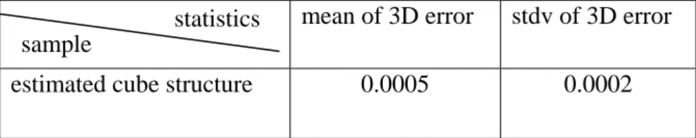
sR where s is a scaling factor and R is a rotation matrix between the output structure and the synthetic model is computed , then the mean and standard deviation of 3D point errors among all the corresponding 3D points are examined. The evaluation of the result is shown in Table 4.1.

Table 4.1. Evaluation of the 3D synthetic cube reconstruction results. mean of 3D error stdv of 3D error estimated cube structure 0.0005 0.0002

Here, we can see the result is nearly perfect in the ideal case.

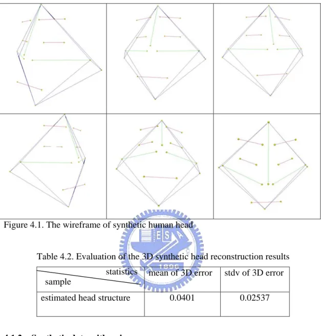
we generate 10 views of another synthetic object which simulates the human head containing 19 points with a dimension of 20×20×10. Figure 4.1 shows the six snap shoots of the wireframe of the synthetic human head. The evaluation of 3D point errors is shown in Table 4.2. The result is nearly perfect.

statistics sample

Figure 4.1. The wireframe of synthetic human head

Table 4.2. Evaluation of the 3D synthetic head reconstruction results mean of 3D error stdv of 3D error estimated head structure 0.0401 0.02537

4.1.2. Synthetic data with noise

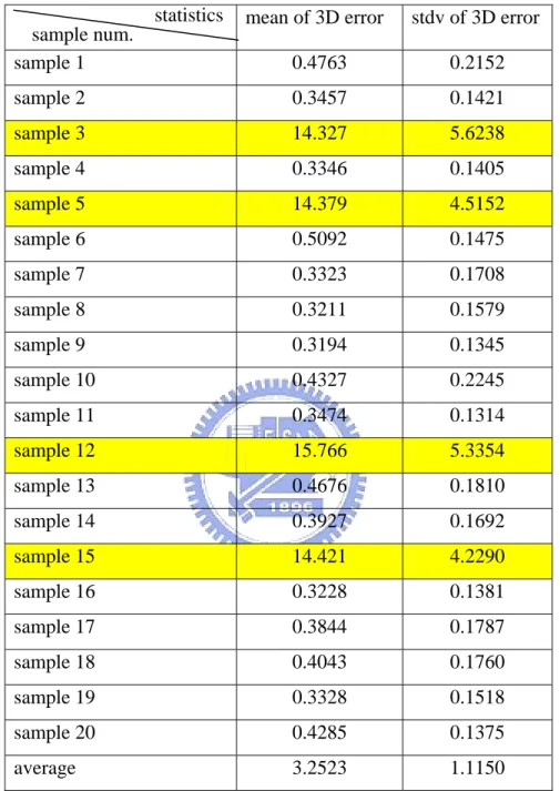
In previous section, we have seen our result is nearly perfect in the ideal case without noise. In the following, we will test the noise tolerance of our system. We add the noise generated by the Gaussian PDF with μ =0 and σ =3 in two directions (horizontal and vertical). We generate 20 noisy copies of the 10-view image stream. We show the cube reconstruction results obtained by two different schemes: one with the statistical IRLS scheme and another without. Table 4.3 lists the average of mean and standard deviation of the 3D point location errors of the cube reconstruction without IRLS scheme, and Table 4.4 lists the average of mean and standard deviation of the 3D point location errors of the cube reconstruction with IRLS scheme(r = 0.95)

statistics sample

Table 4.3 Evaluation of the cube reconstruction results in the noise case without IRLS.

mean of 3D error stdv of 3D error

sample 1 0.4763 0.2152 sample 2 0.3457 0.1421 sample 3 14.327 5.6238 sample 4 0.3346 0.1405 sample 5 14.379 4.5152 sample 6 0.5092 0.1475 sample 7 0.3323 0.1708 sample 8 0.3211 0.1579 sample 9 0.3194 0.1345 sample 10 0.4327 0.2245 sample 11 0.3474 0.1314 sample 12 15.766 5.3354 sample 13 0.4676 0.1810 sample 14 0.3927 0.1692 sample 15 14.421 4.2290 sample 16 0.3228 0.1381 sample 17 0.3844 0.1787 sample 18 0.4043 0.1760 sample 19 0.3328 0.1518 sample 20 0.4285 0.1375 average 3.2523 1.1150 statistics sample num.

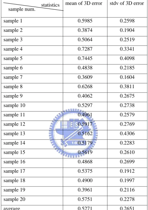
Table 4.4. Evaluation of the cube reconstruction results in the noisy cases with IRLS mean of 3D error stdv of 3D error

sample 1 0.5985 0.2598 sample 2 0.3874 0.1904 sample 3 0.5064 0.2519 sample 4 0.7287 0.3341 sample 5 0.7445 0.4098 sample 6 0.4838 0.2185 sample 7 0.3609 0.1604 sample 8 0.6268 0.3811 sample 9 0.4062 0.2675 sample 10 0.5297 0.2738 sample 11 0.4961 0.2579 sample 12 0.5917 0.2769 sample 13 0.5162 0.4306 sample 14 0.5179 0.2283 sample 15 0.5619 0.2610 sample 16 0.4868 0.2699 sample 17 0.5375 0.1912 sample 18 0.4900 0.1997 sample 19 0.3961 0.2116 sample 20 0.5751 0.2278 average 0.5271 0.2651

From the two experimental results, we can find out there are four crashed samples in a total of 20 samples in the cases without IRLS scheme. We correct the crashed case successfully with the IRLS scheme. The average of mean of 3D error decreases from 3.2523 to 0.5271.

Next, we show the results in synthetic human head reconstruction, also divided into two categories. The first result is without IRLS scheme, and the second result is

statistics sample num.

Table 4.5 Evaluation of the head reconstruction in the noisy cases without IRLS mean of 3D error stdv of 3D error

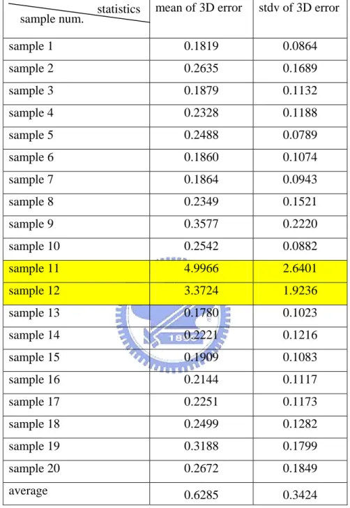
sample 1 0.1819 0.0864 sample 2 0.2635 0.1689 sample 3 0.1879 0.1132 sample 4 0.2328 0.1188 sample 5 0.2488 0.0789 sample 6 0.1860 0.1074 sample 7 0.1864 0.0943 sample 8 0.2349 0.1521 sample 9 0.3577 0.2220 sample 10 0.2542 0.0882 sample 11 4.9966 2.6401 sample 12 3.3724 1.9236 sample 13 0.1780 0.1023 sample 14 0.2221 0.1216 sample 15 0.1909 0.1083 sample 16 0.2144 0.1117 sample 17 0.2251 0.1173 sample 18 0.2499 0.1282 sample 19 0.3188 0.1799 sample 20 0.2672 0.1849 average _{0.6285 0.3424} statistics sample num.

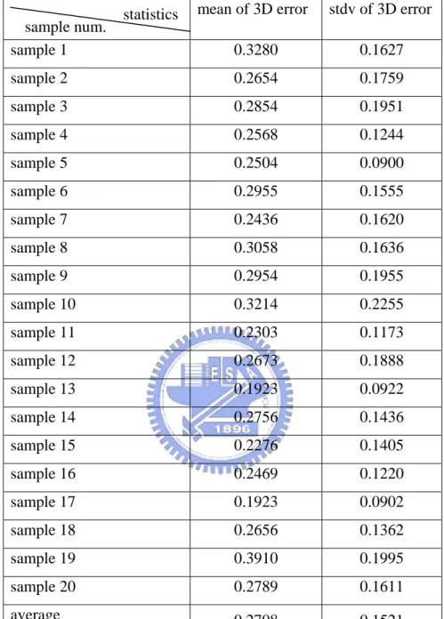
Table 4.6 Evaluation of the head reconstruction results in the noisy cases with IRLS mean of 3D error stdv of 3D error

sample 1 0.3280 0.1627 sample 2 0.2654 0.1759 sample 3 0.2854 0.1951 sample 4 0.2568 0.1244 sample 5 0.2504 0.0900 sample 6 0.2955 0.1555 sample 7 0.2436 0.1620 sample 8 0.3058 0.1636 sample 9 0.2954 0.1955 sample 10 0.3214 0.2255 sample 11 0.2303 0.1173 sample 12 0.2673 0.1888 sample 13 0.1923 0.0922 sample 14 0.2756 0.1436 sample 15 0.2276 0.1405 sample 16 0.2469 0.1220 sample 17 0.1923 0.0902 sample 18 0.2656 0.1362 sample 19 0.3910 0.1995 sample 20 0.2789 0.1611 average _{0.2708 0.1521}

There are two crashed samples in the case without IRLS such that the input data can not achieve an equilibrium automatically. We correct these two samples successfully with the IRLS scheme (r = 0.95) to discard some projection points. The average of mean of 3D error decreases from 0.6285 to 0.2708.

We rely on that the IRLS selects the outlier points which are not consistent with the input data to increase the accuracy of our result. Although in some cases, discarding some projection points will increase the error slightly, it still helps our

statistics sample num.

system to resist the random like noise. In addition, some geometry constraints on the input data should be noticed:

1. Critical motion: the motion only contains the translation or one axis rotation. 2. All of the projection points in some views lie on a plane in the 3D space.

4.2.

Real data with the missing data

4.2.1. Point structure reconstruction of the real object with combination

Due to the viewing constraint, we are usually not capable to reconstruct all points of the real object at the same time. Here, we demonstrate the experiment that we conduct the point structure of the object with two clip segments, then merge these two point structures into one by making use of the overlapping points.

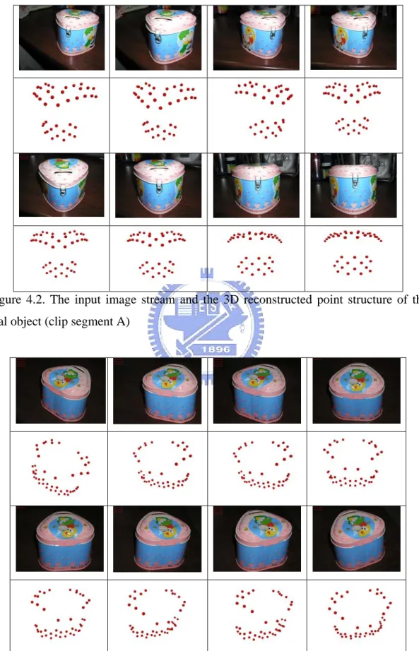
Figure 4.2 shows the input image stream with correspondences and the reconstructed 3D point structure of clip segment A with 41 feature points (structure A), and Figure 4.3 shows the input image stream with correspondences and the reconstructed 3D point structure of clip segment B with 45 feature points (structure B). The clip segment A and the clip segment B have the eight overlapping feature points, and we will use the similarity transformation computed from these eight overlapping points to combine the structure A and the structure B.

Figure 4.2. The input image stream and the 3D reconstructed point structure of the real object (clip segment A)

Figure 4.4 The eight snap shoots of the combined 3D point structure for the structure A and structure B.

4.2.2. Point structure recognition of the human head

We construct a database of five human heads, each containing 19 feature points. A representative image data is shown in Figure 4.5.

Figure 4.5. The images in the human head dataset

Given the above input data, our system is able to reconstruct the 3D point structure. Figure 4.6 shows the six snap shoots of our reconstructed 3D point structure. Table 4.7 is the illustration of our database, each consisting of: the image stream with feature tracking and the corresponding 3D point structure.

Table 4.7. Database of the real human heads with or without eye glasses. Name Input Image

(without eye glasses) 3D Point Structure Input Image (with eye glasses) 3D Point Structure Wu LK Ruping Lee

Chenbc N/A N/A

The evaluation process of the reconstruction results is same as those for the synthetic experiments. Table 4.8 shows the human head recognition result for the five persons subject to a variation in wearing the eye glasses. In this experiment there are 19 head feature points including the four ear feature points. Table 4.9 shows the recognition result for the same case except that four ear feature points are removed (to simulate the case when ears are covered by the hair). From Tables 4.8 and 4.9, all the five persons are correctly recognized no matter whether wearing or not wearing the eye glass or whether four ear feature points are covered or not.

The experiment also indicates that the system can handle the problems of missing points and data noise. In the future, we need to collect a larger database, and

wearing a hat or with bear. Nevertheless, we can construct the 3D geometry for the head, the use of the geometric comparison can resist with the severe figure changes in principle. On the other hand, we may require the person being identified to follow the same general guidelines as she or he files the official papers like the passport photo or ID photo.

Table 4.8. Human head recognition result subject to a variation in wearing the eye glasses. Nineteen feature points including the ear feature points are used.

Wu LK Ruping Lee mean of 3d error mean of 3d error mean of 3d error mean of 3d error Wu 0.2725 0.7034 0.2984 2.4347 LK 0.9480 0.4215 0.3158 3.0554 Ruping 0.8307 0.7614 0.1986 2.2197 Chenbc 1.4882 0.8595 0.5192 3.5336 Lee 1.0998 0.7634 0.3092 1.9284

Table 4.9. Human head recognition result for the same case in Table 4 except that four ear feature points are discarded.

Wu LK Ruping Lee mean of 3d error mean of 3d error mean of 3d error mean of 3d error Wu 0.4809 0.6082 0.2215 1.5746 LK 0.5985 0.3161 0.3281 2.9405 Ruping 0.5952 0.6315 0.1317 1.4417 Chenbc 0.6695 0.8078 0.3147 1.6205 Lee 0.6812 0.7410 0.2884 1.1286 Person

without eye glasses Person with eye glasses

Person

without eye glasses Person with eye glasses

4.2.3. Dense reconstruction of human head

In this section, we continue another experiment to use the fast octree algorithm [1] to do the dense reconstruction of human head with our estimated projection matrix in the Euclidean space. Figures 4.7-4.8 are the five snap shoots of the dense reconstruction results of two persons with the fast octree algorithm. Generally, the reconstructed model captures the real head shape, as indicated by the resemblance between the created one and the real one. However, due to the small camera projection matrix estimation errors the created head contain a bug (a dent in the head) for person 1. Also the quality of the reconstructed head depends on the total number of views used; more views give a better approximation, in particular, those views containing the rapidly varying silhouettes.

Chapter 5. Conclusion and future work

5.1. Conclusion

Our proposed system is capable to handle the missing data and noise. For handling the missing data, our proposed method can deal with directly. For handling the noise, the optimization process of our proposed method has the nature of the bundle adjustment to find the balanced solution such that the effects of random noise cancel out. In some cases where the correct solution results are not possible due to the influence of the outliers, the IRLS feature of our method plays a role to discover these outliers based on the statistical technique. In order to find an Euclidean reconstruction, an iterative auto-calibration procedure using the absolute dual quadric computes an overall rectifying homography even under the situation where the individual estimated camera intrinsic matrix varies across the views because of noise.

From the synthetic data experimental results, our proposed scheme shows the robustness against the random noise generated by the Gaussian PDF. In the real data experimental results, our system can handle mild image noise and missing features.

5.2.

Future work

This thesis exploits the robustness problem of 3D reconstruction of rigid objects. We consider to extend our method to deal with the advanced problems including (1) how to reconstruct structures of multiple objects moving independently [14], (2) how to reconstruct the articulated object whose subparts have different motions. For reconstructing the independently moving object or articulated object, some researchers try to use the statistical methods [15] like expectation maximization algorithm (EM) or the factorization-based methods imposed in articulation constraints [16].

For the application of human head/face recognition, there is a need to test on a larger database for the system evaluation. Besides, the selection of an appropriate representation of the head/face model to deal with variations in the head/face appearance is the essential problem in human head/face recognition.

For a higher accuracy of the reconstruction result, we can achieve by reducing feature correspondence errors.

References:

[1] H. L. Chou, “Constructing 3D Object Models from Image Sequences”, 博士論文, 國立交通大學, 資訊工程學系, 新竹市, 臺灣, 2004.

[2] Y.H. Fang, H.L. Chou, and Z. Chen (2003),”3D Shape Recovery of Complex Objects from Multiple Silhouette Images”, Pattern Recognition Letters 24, 1279-1293.

[3] C. Tomasi and T. Kanade, “Shape and Motion from Image Streams under orthography: A Factorization Method”, International Journal of Computer Vision, vol. 9, no. 2, pp. 137-154, 1992.

[4] C. J. Poelman and T. Kanade, “A Paraperspective Factorization Method for Shape and Motion Recovery,” Proc. Conf. Third European Computer Vision, vol. 2, pp. 97-108, 1994.

[5] R.I. Hartley, “Euclidean Reconstruction from Uncalibrated Views”, Applications of Invariance in Computer Vision, M.Z. Foresyth, ed., pp. 237-256. Berlin Heidelberg: Springer Verlag. 1994.

[6] R. Szelinski and S.B. Kang, ”Recovering 3-D Shape and Motion from Image Streams Using Non-Linear Least Squares,” J. Visual Comm. and Image Representation, vol. 5, no. 1, pp. 10-28, Mar. 1994.

[7] S. Christy and R. Horaud, “Euclidean Shape and Motion from Multiple Perspective Views by Affine Iteration”, IEEE Trans. Pattern Analysis and Machine Intelligence, vol. 18, no. 11, pp.123-141, 1995.

[8] T. Kanade and D. Morris, “Factorization Methods for Structure from Motion,” Philosophical Transactions of the Royal Society of London, vol.A, no. 356, pp. 1,153-1,173, 1998.

[9] H. Aanaes and R. Fisker, “Robust Factorization”, IEEE Transactions on pattern Analysis on Pattern Analysis and Machine Intelligence, vol. 24, no.9, pp. 121-125, 2004.

[10] S. Mahamud, M. Herbert, Y. Omori*, J. Ponce, “Provably-Convergent Iterative Methods for Projective Structure from Motion”, Proc. IEEE Conf. Computer Vision and Pattern Recognition, vol. 1, pp. 1,018-1,025, 2001.

[11] J. Oliensis, “Fast and Accurate Self-Calibration”, Proc. Int' l Conf. Computer Vision, pp. 745-752, 1999.

[12] R. I. Hartley, “In Defense of the Eight-Point Algorithm”, Proc. Fifth Int’ l Conf. Computer Vision, pp. 1,064-1,070, 1995

[13] A. J. Brooker, J. E. Dannis, Jr., P. D. Frank, “A Rigorous Framework for Optimization of Expensive Functions by Surrogates”, Structural Optimization, vol. 17, no. 1, pp. 1-13, 1999.

[14] J. Costeira and T. Kanade, “A Multibody Factorization Method for Independently Moving Objects”, Int’ l J. Computer Vision, vol. 29, no.3, pp. 159-179, 1998.

[15] A.Gruber, Y. Weiss, “Multibody Factorization with Uncertainty and Missing Data Using the EM Algorithm”, Proc. IEEE Conf. Computer Vision and Pattern Recognition. vol. 1, pp. 707-714, 2004

[16] P. Tresadern , I. Reid, “Articulated Structure from Motion by Factorization”, Proc. IEEE Conf. Computer Vision and Pattern Recognition, vol. 2, pp. 1,110-1,115, 2005.

[17] M. Iran , P. Anandan, “Factorization with Uncertainty”, Proc. European Conf. Computer Vision, vol. 1842, pp. 539 – 553, 2000.

[18] W. Triggs, “Auto-calibration and the Absolute Quadric,” Proc. IEEE Conf. Computer Vision and Pattern Recognition, pp. 609-614, 1997.

[19] D. A. Forsyth and J. Ponce, COMPUTER VISION: A MORDERN APPROACH, Pearson Education International, Upper Saddle River, NJ, USA, 2003.

[20] J.H. Wilkinson, C. Reinsch, “Handbook for Automatic Computation”, vol. 2: Linear Algebra, Springer, Heidelberg, 1971.