固定長度眾數區間及其在品質管制上的應用

全文

(1)國立交通大學統計學研究所碩士論文. 固定長度的眾數區間及其在品質管制上的應用 Fixed width mode interval and its application to quality control.. 研究生：林怡均指導教授：陳鄰安. 教授. 中華民國九十三年六月.

(2) 固定長度的眾數區間及其在品質管制上的應用 Fixed width mode interval and its application to quality control.. 研究生：林怡均. Student：Yi Jun Lin. 指導教授：陳鄰安博士. Advisor：Dr. Lin An Chen. 國立交通大學統計學研究所碩士論文. A Thesis Submitted to Institute Statistics College of Science National Chiao Tung University in partial Fulfillment of the Requirements for the Degree of Master in. Statistics June 2004 Hsin-chu, Taiwan, Republic of China. 中華民國九十三年六月.

(3) 固定長度眾數區間及其在品質管制上的應用. 學生：林怡均. 指導老師：陳鄰安教授. 國立交通大學統計學研究所碩士班. 摘. 要. 通用的 Shewhart 管制圖是利用一個統計量 T 的平均數加減 3 倍標準差來做為管制上下限。這套方式應用於所有的分配，不管是對稱或不對稱，以及連續或不連續。我們把 Huang (2003)的眾數區間概念應用於固定長度，但具有最大覆蓋機率的管制圖。對此一區間我們討論了有母數及無母數估計並且做了資料分析。.

(4) Fixed width mode interval and its application to quality control. student：Yi Jun Lin. Advisors：Dr. Lin An Chen. Institute of Statistics National Chiao Tung University. ABSTRACT The popular used Shewhart control chart is choosing a statistic T and setting its upper and lower control limits as T's mean plusing and minusing 3 times of T's standard deviation. This rule has been applied for variables with distributions continuous or discrete and symmetric or asymmetric. We extend the mode interval of Huang (2003) to define the fixed width mode interval which is one having largest coverage probability among the intervals with the same width. Estimation of this new chart has been discussed in parametric and nonparametric techniques. Moreover, a real data analysis has also been provided..

(5) 誌. 謝. 時光飛似，轉眼間研究所求學階段即將結束，謝謝師長們的教導以及同學們的陪伴，讓我經歷了兩年愉快且充實的碩士生涯。首先，我要感謝我的指導老師陳鄰安教授，謝謝老師在忙碌之餘還能撥冗教導我，不厭其煩的指導我在研究時所遇到的問題，使我能如期完成論文。還要感謝已經畢業的博士班黃景業學長，謝謝學長犧牲休假時間，回學校教導我、使我釐清學長論文中的觀念及問題。還要謝謝口試委員對我論文的指導及建議。當然還要感謝研究室的同學欣妤、巧慧、淑珍、政輝、志浩、忠庭、文祥、超毅、小強學長，謝謝他們陪我打球運動、度過學習中的低潮，讓我有健康的身心做研究。此外，還要感謝我的家人以及阿昌給我的支持與鼓勵，讓我能毫無顧慮的求學。最後將此論文獻給我的家人、朋友，以及研究所的同學、學弟妹們。. 林怡均. 謹致于. 國立交通大學統計研究所中華民國九十三年六月.

(6) Contents 中文摘要………………………………………………………………………… i Abstract………………………………………………………………………… ii 誌謝……………………………………………………………………………… iii Content……………………………………………………………………………iv Chapter.1 Introduction……………………………………………………… 1 Chapter.2 Population foxed width interval……………………………. 3. Chapter.3 Statistical inference for fixed width mode interval …………………………………………………………… 7 Chapter.4 Mode interval type control chart…………………………… 10 Chapter.5 Numerical data analysis…………………………………………17 Chapter.6 Nonparametric estimation……………………………………… 18 References……………………………………………………………………… 20 Appendix: Control chart………………………………………………………21.

(7) Fixed Width Mode Interval and Its Application to Quality Control SUMMARY The popular used Shewhart control chart is choosing a statistic T and setting its upper and lower control limits as T ’s mean plusing and minusing 3 times of T ’s standard deviation. This rule has been applied for variables with distributions continuous or discrete and symmetric or asymmetric. We extend the mode interval of Huang (2003) to define the fixed width mode interval which is one having largest coverage probability among the intervals with the same width. Estimation of this new chart has been discussed in parametric and nonparametric techniques. Moreover, a real data analysis has also been provided.. 1. Introduction In statistical applications, we often face two problems of estimating an interval for a random variable or a statistic. In the first problem, we anticipate to find a random interval that covers (usually) a random variable with a given coverage probability. This problem usually is done by the so-called pivotal quantity method. In the second problem, we face the problem of estimating an interval that covers the random variable or statistic in some sense where the two ends of the interval are functions of unknown parameters. There are two main types of this unknown interval. One is setting covering the random variable or statistic with a fixed probability. In this problem, searching one among those with the same coverage probability with shortest width is, in general, a suitable solution. The other one is a certain interval with a fixed width. This interval of the type with fixed width is especially interesting in application in industrial statistics. The popular way in setting an interval of fixed width is selecting T , a statistic T or random variable, with mean µt and standard deviation σt to form the symmetric interval (µt − kσt , µt + kσt ) of width fixed at 2kσt and centered at mean µt where the constant k popular is with value 3. We interpret this with two examples applying in statistical quality control. First, the general form of a Shewhart control chart considers the sample mean or sample range for statistic T and defines the two ends of the interval 1.

(8) 2. as upper control limit (UCL) and lower control limit (LCL) as U CL = µt + 3σt CL = µt . LCL = µt − 3σt where CL represents the central line. Since this control chart may be applied on the manufacturing process no matter what the distribution of the controlling variable is, this interval does not guarantee the coverage probability with a fixed value. Second, using the width of this interval, process capability index is very popular representing the capability of a manufacturing process. For example, consider a random variable X and its standard deviation σ. The simplest version is defined as Cp =. U SL − LSL 6σ. where U SL and LSL, respectively, represent the upper and lower specification limits for the random variable that are determined by engineer. In this example, the index uses the 6σ of the interval (µ − 3σ, µ + 3σ). Consider the problem. The following {(a, a + 6σt ) : a ∈ R},. (1.1). provides the class of whole intervals with the same width 6σt , why should we choose the symmetric one? Two criterions may be appropriate setting for making decision in selection. First, we may treat a fixed width interval as an extension of the traditional concept of location for a distribution of a random variable from a point to an interval. We then expect that it should fulfill several desired eqivariant properties for a location parameter. The traditional Shewhart control charts generally do not satisfy some expected equivariant properties where one is that the constructed intervals may be out of the support of the statistic T . For example, suppose that we have a sample ¯ computed from a random sample X1 , ..., Xn drawn from the distribution mean X √ Gamma(2, 3) where we have its mean µ = 6 and standard deviation σ = 18. We then see that the lower control limit LCL is 6 −. 12.72 √ n. which is less than zero when. n ≤ 4 that makes LCL lie out side the support (0, ∞). Since n ≤ 4 is the very often case in quality control, we need to avoid this in-practical control limits. Second, for ensuring that the manufacturing process is running in appropriateness, a control chart.

(9) 3. should have control limits that work well in two aspects. 1. When the process is in control, we expect not to have data points lie outside the control limits which causes conclusion of possible distributional shift. 2. When the process is out of control, we expect to have more observations lie outside of the control limits that we can detect the fact of distributional shift. Searching a quantile interval that fulfill the two criterions above is our aim in this paper. Extension of the location point of the mode, we define the fixed width interval that maximizes the corresponding coverage probability. From the expectation for being a location interval, we show that it satisfies several desired equivariant properties. ¯ control chart are Its estimation and application in constructing a new Shewhart X addressed. Finally, nonparametric estimation of this interval has also been discussed. We define the mode type interval and show that it satisfies several equivariant properties in Section 2. Examples of mode type intervals for several distributions and their corresponding point estimations are displayed in Section 2. The application of ¯ control chart is introduced in Section 3. Finally, this mode interval to the Shewhart X we introduce a nonparametric estimation for the mode type interval and display several simulation results in Section 4. 2. Population Fixed Width Interval Suppose that we have a random sample X1 , ..., Xn drawn from distribution with p.d.f. f (x, θ). Let T be a statistic based on the random sample or simply the random variable X having p.d.f. f . Let σ 2 be the variance of T , which is usually dependent on θ, and we consider the maximum probability interval of width kσ. Definition 2.1. A kσ fixed width interval is C(θ) = (a∗ (θ), kσ + a∗ (θ)) with a∗ (θ) = argsupa∈R P (a ≤ T ≤ a + kσ). It is well known that the shortest confidence interval with a confidence coefficient may not exist. We then ask if the the kσ fixed width interval which is one of shortest interval exist? The solution provides one reason that it is worthful to be proposed. Theorem 2.2. If a random variable has finite variance σ 2 , then, for k > 0, the kσ fixed width interval exists. Proof. Let’s denote Pa = P (a ≤ T ≤ a + kσ). Note that the set {Pa : a ∈ R} is bounded so that its supremum, denotes it by P ∗ , exists. Let {an : n = 1, 2.3, ...} be a.

(10) 4. set such that p∗ = limi→∞ pai . Since p.d.f. f satisfies f (x) → 0 as x → ∞ or −∞, there exists a value a0 such that −x0 ≤ an ≤ x0 , for all n. Boundness of {an : n = 1, 2, 3, ...} implies that there is a sequence ni such that there is a0 = limi→∞ ani . Suppose that the distribution is continuous. Then obviously a0 is a solution of a∗ . On the other hand, if the distribution is discrete. Then, from the fact that Pa is a step function in a, a∗ has to be the limit of the sequence {ani }. Theorem 2.3. Suppose that the distribution F is symmetric at a value µ, then the kσ fixed width interval is of the form (µ −. k k σ, µ + σ). 2 2. Proof. Consider only that the distribution F is also continuous. Then solution of a satisfies 0=. ∂ (F (a + kσ) − F (a)) = f (a + kσ) − f (a). ∂a. (2.1). However, f (a + kσ) = f (a) if and only if a = µ − k2 σ for symmetric p.d.f. f . We extend the concept of measure of location point (see, for example, Staudte and Sheather (1990, p101)) to the location type interval. Definition 2.4. A measure of fixed width coverage set for F is a set D(X) that satisfies the following conditions: (1). D(X + b) = D(X) + b for b ∈ R. (2). D(aX) = aD(X) for a ∈ R. (3). X ≥ 0 implies D(X) ≥ 0. Not every type of parameterized interval fulfills the properties of measure of fixed width coverage set. Here we show that the kσ fixed width interval does satisfies the conditions of a measure of coverage set. Theorem 2.5. The kσ fixed width interval is a measure of coverage set. Proof. For convenience, redenote a∗ , σ and C(kσ) for random variable X, respectively, by a∗ (X), σX and C(X). To show (1), for c ∈ R, a∗ (X + c) = argsupa∈R P (a ≤ X + c ≤ a + kσX+c ) = argsupa∈R P (a − c ≤ X ≤ a + kσX − c).

(11) 5. where we use the fact that σX+c = σX . We have a∗ (X + c) − c = a∗ (X) which implies a∗ (X + c) = a∗ (X) + c. Then C(X +c) = (a∗ (X +c), a∗ (X +c)+kσX+c ) = (a∗ (X)+c, a∗ (X)+c+kσX ) = C(X)+c. Consider (2). If b > 0, a∗ (bX) = argsupa∈R P (a ≤ bX ≤ a + kσbX ) a a + kbσX = argsupa∈R P ( ≤ X ≤ ) b b where we use the fact that σbX = bσX . We have. a∗ (bX) b. = a∗ (X) which implies. a∗ (bX) = ba∗ (X). Then C(bX) = (a∗ (bX), a∗ (bX) + kσbX ) = b(a∗ (X), a∗ (X) + kσX ) = bC(X). If b < 0, a∗ (bX) = argsupa∈R P (a ≤ bX ≤ a + kσbX ) a − bkσX a = argsupa∈R P ( ≤X≤ ) b b where we use the fact that σbX = −bσX . We have a∗ (X) =. a∗ (bX)−bkσX b. which implies. a∗ (bX) = ba∗ (X) + bkσX . Then C(bX) = (a∗ (bX), a∗ (bX) + kσbX ) = (ba∗ (X) + bkσX , ba∗ (X) + bkσX − bkσX ) = b(a∗ (X), a∗ (X) + kσX ) = bC(X). Condition (3) is induced by the fact that, for X ≥ 0, we have P (a0 ≤ X ≤ a0 + kσ) ≤ P (0 ≤ X ≤ kσ) if a0 < 0. Table 1 Median and mode types interval for binomial distribution (b(12,0.3)).

(12) 6. Length 0 1 2 3 4 5 6 7 8 9 10 11 12. πmed 0.2311 0.4708 0.6293 0.7971 0.8763 0.9475 0.9766 0.9905 0.9983 0.9997 0.9999 0.99999 1.0000. Cmed {4} {3, 4} {3, 4, 5} {2, 3, 4, 5} {2, ..., 6} {1, ..., 6} {1, ..., 7} {0, ..., 7} {0, ..., 8} {0, ..., 9} {0, ..., 10} {0, ..., 11} {0, ..., 12}. πmod 0.2397 0.4708 0.6386 0.7971 0.8763 0.9475 0.9766 0.9905 0.9983 0.9997 0.9999 0.99999 1.0000. Cmod {3} {3, 4} {2, 3, 4} {2, 3, 4, 5} {2, ..., 6} {1, ..., 6} {1, ..., 7} {0, ..., 7} {0, ..., 8} {0, ..., 9} {0, ..., 10} {0, ..., 11} {0, ..., 12}. We call an interval C0 a highest density (HD) interval if f (x) ≥ f (x1 ) for x ∈ C0 , x1 6∈ C0 .. (2.2). Theorem 2.6. Suppose that the underlying distribution is unimodal and continuous. Then a quantile interval C(θ) is a kσ mode interval if and only if it is a width kσ HD interval. Proof. Let C0 be a width kσ HD interval. By the fact that C = (C ∩ C0 ) ∪ (C ∩ C0c ) and C0 = (C0 ∩ C) ∪ (C0 ∩ C c ). Since C and C0 are both width kσ interval, we have width(C ∩ C0c ) = width(C0 ∩ C c ). From (2.2), we also have Z. Z f (x)dx ≥. f (x)dx. C∩C0c. C0 ∩C c. Adding. R C∩C0. f (x)dx to both sides, we further have Z. Z. f (x)dx.. f (x)dx ≥ C0. (2.3). C. However, from the definition of mode interval, strictly inequality in (2.3) can not hold. Then C0 is a width kσ mode interval..

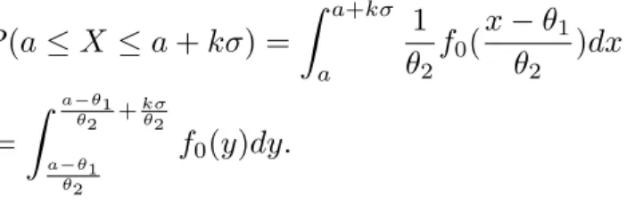
(13) 7. On the other hand, let C = (a, a + kσ) be a kσ mode interval. From (2.1), we have f (a) = f (a + kσ).. (2.4). With (2.4) and the fact that the mode lying in the mode interval, interval C satisfies (2.2). Then C is a width kσ HD interval. 3. Statistical Inferences for Fixed Width Mode Interval Let a fixed width interval be of the form (a1 (θ), a2 (θ)). We also assume that there is a random sample X1 , ..., XN available. Consider θˆ as an estimator of θ. In this section, we will develop statistical inference procedures for the fixed width interval when the interval is a function of unknown parameter θ and a random sample from the underlying distribution is available. The simplicity of the expression of the fixed width mode interval determines the estimation technique. Suppose that a distribution Fθ makes the mode interval in the form (a1 (θ)c0 , a1 (θ)c0 + kσ). (3.1). where c0 is the only fact that is determined by the maximization problem in Definition 2.1 in terms of a distribution F0 which is free of parameter θ. Then as long as we have estimators θˆ and σ ˆ respectively for θ and σ the estimator of the mode interval may ˆ 0 , a1 (θ)c ˆ 0 + kˆ be set as Cˆ = (a1 (θ)c σ ). The distribution belonging to the family of location-scale family is the one with this advantage. In the following, we presents the fixed width mode interval for several distributions that belong to the location-scale family. Theorem 3.1. Let X be a random variable with distribution in the family of continuous location-scale distributions with p.d.f. of the form f (x, θ1 , θ2 ) = parameter space θ1 ∈ R and θ2 > 0 has kσ mode interval of the type (a∗ , a∗ +. kσ ) θ2. where a∗ = argsupa∈R P (a ≤ X0 ≤ a + and X0 =. X−θ1 θ2 .. kσ ). θ2. x−θ1 1 θ2 f0 ( θ2 ). with.

(14) 8. Proof. The proof is obvious from the fact that Z P (a ≤ X ≤ a + kσ) = Z =. a a−θ1 θ2. + kσ θ. a−θ1 θ2. 2. a+kσ. 1 x − θ1 f0 ( )dx θ2 θ2. f0 (y)dy.. The benifit of location-scale family is that the mode interval is explicitly displayed in terms of α∗ and parameter θ and then we may easily develop the estimator of coverage interval through the existed theorems for statistical inferences for parameter θ. Exponential distribution: Consider the case that the random sample is drawn from a right skewed exponential distribution with p.d.f. f (x) =. 1 − x−` e θ I(` < x < ∞). θ. The kσ fixed width interval is C(θ) = (`, ` + kθ). Proof. For this distribution, we may see that standard deviation is σ = θ and P (a < X < a + kσ) = e−. a−` θ. 1 − e−kσ/θ > 0 and e−. (1 − e−kσ/θ ). Then the result is implied from the facts that. a−` θ. is a decreasing function of a on [`, ∞). ¤. Table 2 Comparison of coverage probabilities of median and mode types intervals for the Exponential distribution with the coverage probabilities for normal distribution k 1.0 2.0 3.0 4.0 5.0 6.0 7.0. πmed λ = 0.3 0.419 0.830 0.924 0.956 0.977 0.989 0.996. πmod 0.644 0.865 0.954 0.988 0.999 1.000 1.000. πmed λ=3 0.417 0.830 0.923 0.956 0.977 0.989 0.996. πmod 0.643 0.865 0.954 0.988 0.999 1.000 1.000. πnor Normal 0.382 0.682 0.866 0.954 0.987 0.997 0.999. For the point estimation, in case that we have a random sample X1 , ..., Xn drawn ¯ since X ¯ is the from this exponential distribution, we may consider Cˆ = (`, ` + k X) best estimator of θ..

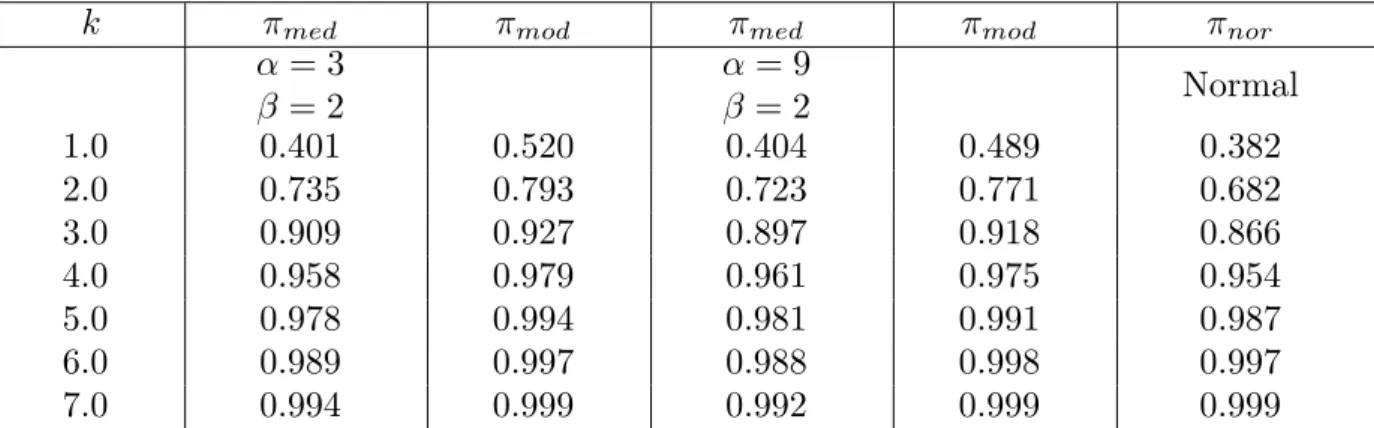
(15) 9. On the other hand, one distribution highly asymmetric skewed to the left that has p.d.f. of the form f (x) =. 1 x−` e θ I(−∞ < x < `). θ. We may also see that the kσ fixed width interval is C(θ) = (` − kθ, `) ¯ `). where its estimator may be set as Cˆ = (` − k X, Gamma distribution: Suppose that X has distribution Gamma( 2` , θ). Since E(X) =. `θ 2. and V ar(X) =. `θ 2 2 ,. Cmed. then the kσ fixed width interval is. `θ k =( − θ 2 2. r. ` `θ k , + θ 2 2 2. r. ` ) 2. and the mode type 2kσ fixed width interval is a∗0 a∗0 θk √ θ, θ + 2`) 2 2 2 √ where a∗0 solves supa∈R P (a ≤ χ2 (`) ≤ a +qk 2`). Proof of mode type interval: Since σ = 2` θ, the kσ fixed width interval is C(θ) = q (a∗ , a∗ + k 2` θ) where a∗ satisfies the followings Cmod (θ) = (. r. ` θ) 2 √ 2a 2X 2a + k 2`). ≤ ≤ = argsupa∈R P ( θ θ θ ∗. a = argsupa∈R P (a ≤ X ≤ a + k. Since. 2X θ. has χ2 distribution with degrees of freedom `, the theorem is followed. ¤. The coverage probabilities of the median type and mode type 2kσ fixed width interval are, respectively, r r ` `θ k ` `θ k ) + θ ≤X≤ πmed = P ( − θ 2 2 2 2 2 2 r r ` ` ) ≤ χ2 (`) ≤ ` + k = P (` − k 2 2 and. √ πmod = P (a∗0 ≤ χ2 (`) ≤ a∗0 + k 2`)..

(16) 10. Table 3 Comparison of coverage probabilities of median and mode types intervals for the Gamma distribution with the coverage probabilities for normal distribution k 1.0 2.0 3.0 4.0 5.0 6.0 7.0. πmed α=3 β=2 0.401 0.735 0.909 0.958 0.978 0.989 0.994. πmod 0.520 0.793 0.927 0.979 0.994 0.997 0.999. πmed α=9 β=2 0.404 0.723 0.897 0.961 0.981 0.988 0.992. πmod. πnor Normal. 0.489 0.771 0.918 0.975 0.991 0.998 0.999. 0.382 0.682 0.866 0.954 0.987 0.997 0.999. Let’s turn to the situation that a distribution does not belong to the location-scale family. It is then quite often that the fixed kσ mode interval may ne be formulated in ˆ the convenient form of (3.1). In this situation, we propose to estimate it as Cˆ = C(θ) simply replacing the distribution Fθ of X by Fθˆ where θˆ is a suitable estimator of θ. In the following, we present a case of underlying Poisson distribution. Poisson distribution: Let X be a random variable with Poisson distribution having p.d.f. of the form f (x, λ) =. λx e−λ I(x = 0, 1, 2, ...). x!. The variance of this distribution is λ so that the kσ mode interval is C(λ) = (a(λ), a(λ)+ √ k λ) with a(λ) = argsupa≥0. √ a+k Xλ x=a. λx e−λ . x!. ¯ where X ¯ is the sample When λ is unknown, we may estimate C(λ) by Cˆ = C(X) mean of the available random sample X1 , ..., Xn . 4. Mode Interval Type Control Chart Let T be a statistic based on a random sample from a distribution F with population mean µt and population variance σt2 . The general theory of Shewhart control chart is considering the mean µt as the central line and the two lines with distance 2kσt for.

(17) 11. some k > 0 as the upper and lower control limits as U CL = µt + kσt CL = µt LCL = µt − kσt In practice, the most popular setting of value k is 3. Basically, the Shewhart control is an interval with fixed width 2kσt . Inheriting the requirement of the fixed width 2kσt , it is reasonable to consider the limits of the fixed width 6σt mode interval as the control limits, that is, we define the general form of mode interval type fixed width Shewhart control limits as U CLmod = 2kσt + a∗ (θ) LCLmod = a∗ (θ) In practice of quality control, usually we assume that there is a history record of m samples Xj1 , Xj2 , ..., Xjn , j = 1, ..., m drawn from a distribution F available to construct the control limits. Let µ ˆtj , σ ˆtj and a ˆ∗j (θ) are, based on jth random sample Pm 1 Xj1 , Xj2 , ..., Xjn , estimators of µt , σt and a∗ (θ). By letting µ ˆt = m ˆtj , σ ˆt = j=1 µ Pm Pm ∗ 1 1 ∗ ˆtj and a ˆ (θ) = m j=1 a ˆj (θ), the estimated Shewhart control chart and j=1 σ m mode interval type Shewhart control chart are, respectively, with limits U CL = µ ˆt + kˆ σt CL = µ ˆt LCL = µ ˆt − kˆ σt and U CLmod = 2kˆ σt + a ˆ∗ (θ) LCLmod = a ˆ∗ (θ) In application of this new control chart for on-line process surveillance, if the sample values of statistic T fall within the control limits LCLmod and U CLmod and do not exhibit any systematic pattern, we say the process is in control at the level indicated by the chart..

(18) 12. Exponential Distribution Let X1 , ..., Xn be a random sample drawn from the exponential distribution with p.d.f.. 1 −x e θ I(x > 0). θ ¯ ¯ Consider the X-chart. The Shewhart control X-chart is f (x, θ) =. θ U CLmed = θ + k √ n CLmed = θ θ LCLmed = θ − k √ n ¯j = By letting X ¯ X-chart is. 1 n. Pn. =. i=1 Xji and X=. 1 m. U CLmed. Pm j=1. ¯ j , the estimated Shewhart control X =. X =X +k √ n =. =. CLmed =X LCLmed. =. X =X −k √ n =. ¯ On the other hand, the coverage probability of the Shewhart control X-chart may be derived in the following θ ¯ ≤ θ + k √θ ) πmed = P (θ − k √ ≤ X n n n X θ θ Xi ≤ n(θ + k √ )) = P (n(θ − k √ ) ≤ n n i=1 k k = P (n(1 − √ ) ≤ Y ≤ n(1 + √ )) n n where Y ∼ Gamma(n, 1). ¯ The mode type Shewhart control X-chart is θ U CLmod = 2k √ + a∗ (θ) n ∗ LCLmod = a (θ).

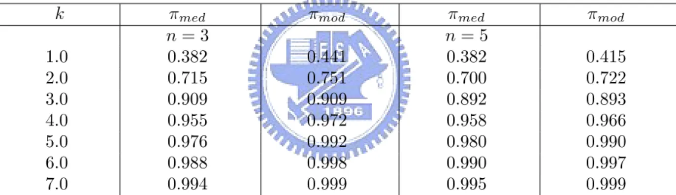
(19) 13. where a∗ (θ) may be derived in the following ¯ ≤ 2k √θ + a) a∗ (θ) = argsupa P (a ≤ X n Pn Xi a 2k a = argsupa P (n ≤ i=1 ≤ n( √ + )). θ θ n θ 2k By letting b∗ = argsupb P (nb ≤ Y ≤ n( √ + b)), we have a∗ = θb∗ . The alternative n ¯ form of the mode type Shewhart control X-chart is. θ U CLmod = 2k √ + θb∗ n ∗ LCLmod = θb Table 4 Comparison of coverage probabilities of median and mode types control limits for the Exponential distribution k. πmed n=3 0.382 0.715 0.909 0.955 0.976 0.988 0.994. 1.0 2.0 3.0 4.0 5.0 6.0 7.0. πmod. πmed n=5 0.382 0.700 0.892 0.958 0.980 0.990 0.995. 0.441 0.751 0.909 0.972 0.992 0.998 0.999. πmod 0.415 0.722 0.893 0.966 0.990 0.997 0.999. ¯ The estimated mode type Shewhart control X-chart is =. U CLmod. = X = 2k √ + X b∗ n =. LCLmod =X b∗ ¯ The coverage probability of the mode type Shewhart control X-chart is 2k πmod = P (nb∗ ≤ Y ≤ n( √ + b∗ )). n Gamma distribution Let X1 , ..., Xn be a random sample drawn from the distribution ¯ control chart. Since X ¯ has mean `θ and Gamma( ` , θ). Consider the Shewhart X 2. 2.

(20) 14. variance. `θ 2 2n ,. ¯ control chart is the median type Shewhart X r `θ ` U CLmed = + kθ 2 2n `θ CLmed = 2 r `θ ` LCLmed = − kθ 2 2n. ¯ control chart is The sample type Shewhart X =. =. =. =. r. U CLmed =X +k X. ` 2n. =. CLmed =X LCLmed =X −k X. r. ` 2n. ¯ control chart is The coverage probability of the median type Shewhart X r r `θ ` `θ ` ¯≤ πmed = P ( − kθ ≤X + kθ ) 2 2n 2 2n r r ` ` ` ` = P (n( − k ) ≤ Y ≤ n( + k )). 2 2n 2 2n Pn Xi ¯ For deriving the mode type X control chart, by letting Y = i=1 , and setting θ r. ¯ ≤ a + 2kθ ` ) a (θ) = argsupa P (a ≤ X 2n r `n ), b∗ = argsupb P (b ≤ Y ≤ b + 2k 2 ∗. we have a∗ =. θb∗ n .. ¯ control chart is The mode type Shewhart X r U CLmod = kθ LCLmod =. 2` θb∗ + n n. θb∗ . n. Table 5 Comparison of coverage probabilities of median and mode types control limits for the Gamma distribution Gamma(2, 2).

(21) 15. k 1.0 2.0 3.0 4.0 5.0 6.0 7.0. πmed n=3 0.382 0.697 0.888 0.959 0.981 0.991 0.996. πmod. πmed n=5 0.382 0.691 0.879 0.958 0.983 0.993 0.997. 0.409 0.715 0.888 0.964 0.990 0.997 0.999. πmod 0.398 0.702 0.880 0.960 0.989 0.997 0.999. ¯ control chart is The sample mode type Shewhart X =. r. U CLmod = 2k X. =. 2 2Xb∗ + n` n`. =. LCLmod. 2Xb∗ = . n`. ¯ control chart is The coverage probability of the mode type Shewhart X r πmod = P (b∗ ≤ Y ≤ b∗ + 2k. n` ). 2. Poisson distribution Let X1 , ..., Xn be a random sample drawn from the distribution ¯ control chart. Since E(X) ¯ = λ and V ar(X) ¯ = λ. P oisson(λ). Consider also the X n. the median type Shewhart control chart is r U CLmed = λ + k CLmed = λ. r. LCLmed = λ − k. λ n λ n. The sample type Shewhart control chart is s =. U CLmed =X +k. =. X n. =. CLmed =X =. LCLmed =X −k. s. =. X n.

(22) 16. ¯ control chart is The coverage probability of the median type Shewhart X r r λ ¯ ≤ λ + k λ) πmed = P (λ − k ≤X n n r r λ λ = P (n(λ − k ) ≤ Y ≤ n(λ + k )) n n Pn where we let Y = i=1 Xi ∼ P oisson(nλ). ¯ control chart is The mode type Shewhart X r λ U CLmod = a∗ + 2k n ∗ LCLmod = a where a∗ satisfies. r. λ n r λ = argsupa P (na ≤ Y ≤ n(a + 2k )). n ¯ control chart is The sample type mode type Shewhart X s = = X ∗ U CLmod = a (X) + 2k n. ¯ ≤ a + 2k a = argsupa P (a ≤ X ∗. =. LCLmod = a∗ (X) =. where a∗ (X) satisfies. s. =. X a (X) = argsupa P (na ≤ Y ≤ n(a + 2k )). n We here display a comparison of coverage probabilities of median type and mode ¯ charts under the Poisson distribution with sample size n = 3 type X ∗. =. Table 6 Comparison of coverage probabilities of median and mode types control limits for distribution P oisson(0.5) (n=3) k 1.0 2.0 3.0 4.0 5.0 6.0 7.0. πmed 0.585 0.585 0.934 0.934 0.981 0.995 0.995. (LCL, U CL)med (0.3, 0.704) (0.092, 0.908) (0.0, 1.112) (0.0, 1.316) (0.0, 1.521) (0.0, 1.725) (0.0, 1.929). πmod 0.585 0.808 0.934 0.981 0.999 0.999 0.999. (LCL, U CL)mod (0.3, 0.708) (0.0, 0.816) (0.0, 1.225) (0.0, 1.633) (0.0, 2.041) (0.0, 2.449) (0.0, 2.858).

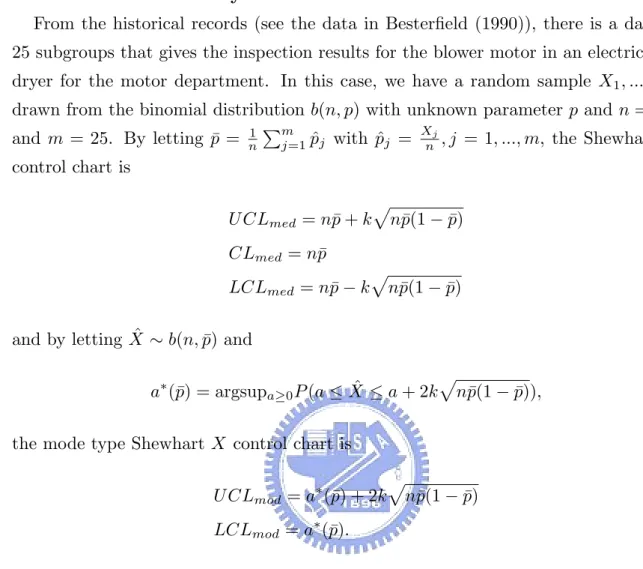
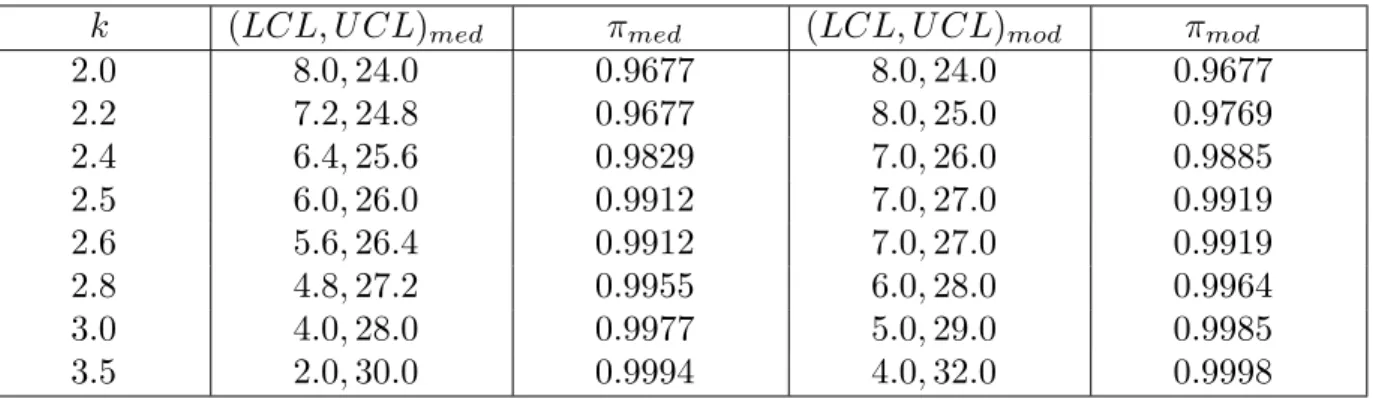
(23) 17. 5. Numerical Data Analysis From the historical records (see the data in Besterfield (1990)), there is a data of 25 subgroups that gives the inspection results for the blower motor in an electric hair dryer for the motor department. In this case, we have a random sample X1 , ..., Xm drawn from the binomial distribution b(n, p) with unknown parameter p and n = 300 Pm X and m = 25. By letting p¯ = n1 j=1 pˆj with pˆj = nj , j = 1, ..., m, the Shewhart X control chart is U CLmed = n¯ p+k CLmed = n¯ p LCLmed = n¯ p−k. p n¯ p(1 − p¯). p n¯ p(1 − p¯). ˆ ∼ b(n, p¯) and and by letting X ˆ ≤ a + 2k a∗ (¯ p) = argsupa≥0 P (a ≤ X. p n¯ p(1 − p¯)),. the mode type Shewhart X control chart is U CLmod = a∗ (¯ p) + 2k. p n¯ p(1 − p¯). LCLmod = a∗ (¯ p). Table 7 Median and mode control chart for binomial distribution k 2.0 2.2 2.4 2.5 2.6 2.8 3.0 3.5. (LCL, U CL)med 0.794, 10.00 0.333, 10.46 −0.126, 10.92 −0.126, 10.92 −0.587, 11.38 −1.047, 11.84 −1.508, 12.30 −2.659, 13.45. πmed 0.9742 0.9742 0.9785 0.9910 0.9910 0.9910 0.9965 0.9987. (LCL, U CL)mod 1.00, 10.0 1.00, 11.0 1.00, 11.0 1.00, 12.0 1.00, 12.0 1.00, 12.0 0.00, 13.0 0.00, 16.0. πmod 0.9742 0.9967 0.9867 0.9922 0.9922 0.9922 0.9987 0.9999. We display a graph of the estimated control chart in Figure 1. In statistical quality control, the number of defects, c, arises probabilitically according to the Poisson distribution. Suppose that we have a random sample c1 , ..., cm.

(24) 18. obeying this distribution. By denoting c¯ =. 1 m. Pm. i=1 ci ,. the Shewhart c control chart. has control limits √ U CLmed = c¯ + k c¯ CLmed = c¯. √ LCLmed = c¯ − k c¯. On the other hand, the mode type Shewhart c control chart has control limits as √ U CLmod = a∗ (¯ c) + 2k c¯ LCLmod = a∗ (¯ c) √ √ where a∗ (¯ c) = argsupa≥0 P (a ≤ cˆ ≤ a + 2k c¯) where cˆ ∼ P oisson( c¯). Consider the process of the installation of front and rear bumpers on automobiles. In this automobile manufacturer, all autos were inspected for the bumper installation process. The numbers c1 , ..., cm of defects were recorded from shift to shift. For detail description of the data and defects, please see Devor, Chang, and Sutherland (1992). From the data of m = 25 samples, the mean of defects c¯ = 16. We list the two computed control limits in the following table. Table 8 Median and mode control chart for bumper infects k 2.0 2.2 2.4 2.5 2.6 2.8 3.0 3.5. (LCL, U CL)med 8.0, 24.0 7.2, 24.8 6.4, 25.6 6.0, 26.0 5.6, 26.4 4.8, 27.2 4.0, 28.0 2.0, 30.0. πmed 0.9677 0.9677 0.9829 0.9912 0.9912 0.9955 0.9977 0.9994. (LCL, U CL)mod 8.0, 24.0 8.0, 25.0 7.0, 26.0 7.0, 27.0 7.0, 27.0 6.0, 28.0 5.0, 29.0 4.0, 32.0. πmod 0.9677 0.9769 0.9885 0.9919 0.9919 0.9964 0.9985 0.9998. We also display an estimated control chart in Figure 2. 6. Nonparametric Estimation In the previous work in this paper, the observations were assumed to come from some underlying distribution, whose general form is assumed known. If these assumptions about the shape of the distribution are not made, then nonparametric methods to.

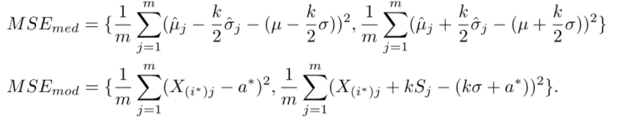
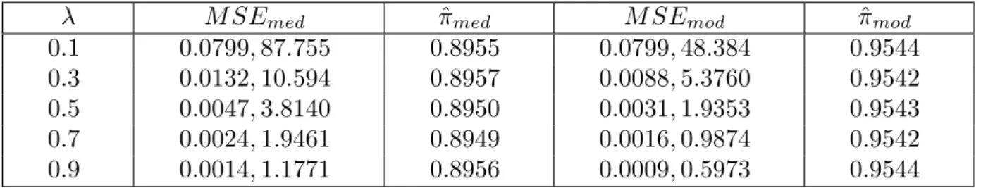
(25) 19. estimate the fixed width mode interval Cmod = (a∗ , kσ + a∗ ) must be used. Besides the nonparametric estimation of mode interval Cmod , we also simulate the efficiency of the mode interval Cmod comparing with median type interval. As we have defined earlier, the median type interval is Cmed = (µ− k2 σ, µ+ k2 σ). For further study, we here also consider another type of median type interval as Cmed2 = (F −1 (α0 ), kσ+F −1 (α0 )) with F −1 (α0 ) satisfying P (X ≤ F −1 (α0 )) = P (X ≥ kσ + F −1 (α0 )).. ¯ = 1 Pn Xi Let X1 , ..., Xn be a random sample from a distribution F , we let X i=1 n Pn 1 2 1/2 ¯ and S = ( n−1 i=1 (Xi − X) ) , the, respectively, sample mean and sample standard deviation, and X(1) , X(2) , ..., X(n) be the corresponding order statistics. Let n∗ = max{ni = number of observations in [X(i) , X(i) + kS], i = 1, ..., n} and let i∗ be the index i such that number of observations in [X(i) , X(i) + kS] is equal to n∗ . We then define the estimate of the kσ mode interval by Cˆmod = [X(i∗ ) , X(i∗ ) + kS]. ∗. The corresponding coverage percentage estimate is π ˆmod = nn . The ordinary Shewhart control chart is Cˆmed = (ˆ µ− kσ ˆ, µ ˆ + kσ ˆ ) where its corresponding coverage percentage is π ˆmed =. 2 2 ˆmed number of observations in C . n. We consider a simulation with replication m = 10, 000. For each replication, we draw a random sample X1 , ..., Xn of sample size n = 50 from a distribution F . Besides the estimated coverage probabilities, we also setting the following vector type mean squares errors (MSE): m. m. M SEmed. k k 1 X k k 1 X ˆj − (µ + σ))2 } (ˆ µj + σ ˆj − (µ − σ))2 , (ˆ µj − σ ={ 2 2 m j=1 2 2 m j=1. M SEmod. 1 X 1 X (X(i∗ )j + kSj − (kσ + a∗ ))2 }. (X(i∗ )j − a∗ )2 , ={ m j=1 m j=1. m. m. The first we consider the exponential distribution with pdf f (x, λ) = λe−λx , x > 0 and we display both the MSE’s and the estimated coverage probabilities. Table 9 MSE’s and coverage percentages for Exponential distribution.

(26) 20. λ 0.1 0.3 0.5 0.7 0.9. M SEmed 0.0799, 87.755 0.0132, 10.594 0.0047, 3.8140 0.0024, 1.9461 0.0014, 1.1771. π ˆmed 0.8955 0.8957 0.8950 0.8949 0.8956. M SEmod 0.0799, 48.384 0.0088, 5.3760 0.0031, 1.9353 0.0016, 0.9874 0.0009, 0.5973. π ˆmod 0.9544 0.9542 0.9543 0.9542 0.9544. We have two conclusions: (a). The MSE’s of Cmod for estimation of its two ends are uniformly smaller or equal to the corresponding MSE’s of Cmed . This indicates that the location of mode interval is relatively easy to estimate than the location of median interval. (b). The estimated coverage probabilities based on Cmod are also significantly larger than those based on Cmed . Table 10 Coverage percentages for distribution Beta(α, β) β 1 3 5 7 9. π ˆmed α=3 0.9032 0.8642 0.8709 0.8791 0.8855. π ˆmod 0.9309 0.8942 0.8986 0.9047 0.9092. π ˆmed α = 10 0.9099 0.8875 0.8728 0.8682 0.8669. π ˆmod 0.9419 0.9104 0.8997 0.8956 0.8949. References Besterfield, D. H. (1990). Quality Control. Prentice Hall: New Jersey. DeVor, R. E., Chang, T.-H. and Sutherland, J. W. (1992). Statistical Quality Design and Control. Prentice Hall: New Jersey. Huang, J.-Y. (2003). Mode interval and its application to construct a new Shewhart control chart. Ph.D. thesis, National Chiao Tung University. Staudte, R. G. and Sheather, S. J. (1990). Robust Estimation and Testing, Wiley: New York..

(27) Figure.1 np control chart for blower motor data. Figure.2 C control chart for rear bumper data.

(28)