在微陣列資料上利用基因分群以減少冗贅之基因選取方法

國

立

交

通

大

學

統計學研究所

碩

士

論

文

在微陣列資料上利用基因分群以減少冗贅之基因選取方法

Redundancy-Reducing Feature Selection from Microarray

Data Based on Gene-Grouping

研 究 生：張寶文

指導教授：洪志眞 教授

洪慧念 教授

在微陣列資料上利用基因分群以減少冗贅之基因選取方法

Redundancy-Reducing Feature Selection from Microarray

Data Based on Gene-Grouping

研 究 生：張寶文 Student：Bao-Wen Chang

指導教授：洪志眞 博士 Advisors：Dr. Jyh-Jen Horng Shiau

洪慧念 博士 Dr. Hui-Nien Hung

國 立 交 通 大 學

統計學研究所

碩 士 論 文

A Thesis

Submitted to Institute of Statistics College of Science

National Chiao Tung University in Partial Fulfillment of the Requirements

for the Degree of Master

in Statistics June 2004

Hsinchu, Taiwan, Republic of China

在微陣列資料上利用基因分群以減少冗贅之基因選取方法

研究生：張寶文 指導教授：洪志眞 博士

洪慧念 博士

國立交通大學統計學研究所

摘 要

微陣列資料集通常包含數千個基因，但只有數十個樣本。這種所謂“大

p (基因)，小 n (樣本)＂的特性會為統計分析帶來一些困難。基因選取是處

理這類問題的一種典型方法。其中，Filters 和 wrappers 是兩種常用的基因

選取方法。Filters 利用一個排序準則來判斷一個基因是否被選取；因此，這

種方法在計算上非常快速，但可能選到高度相關的基因而造成冗贅。另一

方面，wrappers 通常能夠選取一個不冗贅的基因子集但卻需要龐大的運算

量。這篇研究中採用上述二種方法的組合。我們先根據一個排序準則過濾

掉對分類無益的基因，再利用 K-means 分群演算法對其餘基因分群以避免

冗贅。然後，應用 Guyon et al. (2002) 所提出的 SVM-RFE 基因選取方法於

自每群選出的候選基因。最後，我們利用所提出的方法來分析三個常見的

癌症資料集。其結果顯示，當選出的基因數目少時，我們的方法表現地比

所討論的三種 filters 好。

Redundancy-Reducing Feature Selection from Microarray

Data Based on Gene-Grouping

Student：Bao-Wen

Chang

Advisors：Dr. Jyh-Jen Horng Shiau

Dr. Hui-Nien Hung

Institute of Statistics

National Chiao Tung University

ABSTRACT

A microarray dataset contains thousands of genes but only tens of subjects in general. This so-called “large (gene), small (subject)” feature brings about some difficulties to statistical analysis. Gene selection is a typical approach to deal with this problem. There are two conventional gene selection methods, filters and wrappers. Filters judge whether a gene should be selected based on a ranking criterion; therefore, they are very fast in computation but might select highly correlated genes that give rise to redundancy. On the other hand, wrappers usually select a small set of non-redundant genes but require extensive computation. A combination of these two methods is adopted in this study. We first filter out irrelevant genes according a ranking criterion and then group the rest to avoid redundancy via K-means clustering algorithm. Then, the SVM-RFE gene selection method proposed by Guyon et al. (2002) is applied to a list of candidate genes selected from each cluster. Three popular cancer data sets are analyzed by means of the proposed method. The results show that the proposed method performs better than three filter methods under study when the number of selected genes is small.

誌 謝

這篇論文的完成除了自己的努力及堅持外，首要感謝我的兩位指導老

師，有了洪志真教授的耐心指導及洪慧念教授的指點迷津，讓我的論文能

夠順利完成。同時，也謝謝曾參與討論的翠英、淑淨、巧慧及超毅，有了

他們的參與使我能更清楚問題。

這兩年，學習到不少專業知識及處事哲學，也結交了許多好友，除了

上述提及的同學外，還有多才多藝的崢珮、養生有道的 kobe、熱心的 ken、

最有義氣的華勝、少根筋的志浩、小氣的 ming 及大胖政輝；此外，也謝謝

常常一起打球的牛哥及其平時給予我的教誨，感謝這些人使我的研究所生

涯更為豐富、有趣，也希望沒有遺漏。

最後，感謝家人及男友給我的支持和鼓勵讓我能勇於面對困境。

張 寶 文 謹誌于

國立交通大學統計學研究所

中華民國九十三年六月

Contents

Chinese Abstract ………. i

English Abstract ……….... ii

Acknowledgment ……….. iii

Contents ……… iv

1. Introduction ………... 1

2. Literature Review ………. 4

3. Methodology – A Combined Gene Selection Scheme ………… 9

3.1

K-means ………...… 9

3.2

Support Vector Machines ………... 10

3.3

The Proposed Gene Selection Scheme ………... 14

4. Data Analysis ………... 17

4.1

Leukemia Data ………... 17

4.2

Colon Cancer Data ………. 18

4.3

Breast Cancer Data ………. 19

5. Conclusions and Future Research ………... 21

References ……… 23

1. Introduction

Cancer classification is an important issue in medical community. The development of microarray technology enables biologists to observe the expression levels of thousands of genes simultaneously in a single array. Microarray techniques take the clinical diagnosis from morphology to molecular biology. Several microarray datasets on a variety of cancers are

publicly available on the Internet. Typically, the dataset is organized as a matrix X_{p n×} where

the element x_ij represents the expression level of the th gene of the th subject. Subjects

are classified into classes such as normal tissues versus cancer tissues, or different types of a certain disease. The challenge we are confronted here is how to distinguish cancer tissues from normal tissues when tremendous measurements of gene expression levels are given for these tissues.

i j

Several statistical issues have been encountered in gene expression data analysis, including image analysis, experimental design, data preprocessing, clustering, classification, gene (feature) selection and so on (Nadon and Shoemaker (2002); Sebastiani et al. (2003)). Many statistical methods used in analyzing microarray data are based on machine learning methodologies. Supervised learning and unsupervised learning are frequently used in machine learning. Basically, supervised learning is to predict an outcome (response) based on a set of features of an object. More specifically, we use the outcomes and feature measurements of samples in a set of training data to build a prediction model (or “learner”), e.g., by least squares methods. Support Vector Machines (SVMs) is also a popular method in recent years, especially in classification. It is called “supervised” because the outcomes in training data are used to guide the learning process. On the other hand, unsupervised learning (or “learning without a teacher”) observes only feature measurements and has no outcome measurements. Its task is to gain some understanding of data. For example, clustering is a typical

unsupervised learning technique.

In this study, we only discuss the two-class classification problem in which classes are

labeled as { ,+ −} or { 1, 1}.+ − That is, each subject x_j is accompanied by a corresponding outcome (response) y_j∈ + −{ 1, 1}. With these class-labeled data as a training set, an unknown-class subject can be classified by means of statistical methods described above. Unfortunately, a microarray dataset usually contains thousands of genes but only tens of subjects in general. This so-called “large small ” feature brings about some difficulties to statistical analysis. More specifically, we have too many genes relative to the number of subjects. It means that we have to deal with a statistical problem with a large number of variables (genes) and a small number of observations (subjects). Under such circumstances, we may get an overfitting solution, that is, a decision function that performs well for training data but poorly for test data. It is probably because the great part of the variables (genes) is irrelevant or even becomes noise to the problem. This overfitting problem is well known in machine learning. The typical approach to overcome this problem is to reduce the dimensionality of the feature space.

,

p n

Feature (gene) selection is a commonly used method for dimension reduction in classification problems. By means of gene selection, we not only improve the accuracy of classification by reducing the dimensionality but also reduce the computational cost. Furthermore, it is believed that there are only a handful of genes that dominate a certain disease. Feature (gene) selection grubs up a list of candidate genes that is interpretable enough to help identify, say, cancer tissues from normal tissues. The main objective of this study is to pick some crucial genes to help classification, or even disease detection, cure, and prevention.

There are two general approaches to feature (gene) selection: filters and wrappers. Filters judge whether a feature (gene) should be selected based on its discriminating power, while wrappers select features (genes) according to the accuracy of the learning method. If we

choose filters to select genes, we might get highly correlated genes that give rise to redundancy. This redundancy is useless to the advance of classification accuracy and may skew the results or even lead to misclassifications. On the other hand, wrapper methods can often obtain a small set of non-redundant features (genes) but require extensive computation to search for an adequate set of features (genes).

We will address gene selection problem by combining the two approaches described above. First, filter out features (genes) with little or no effects in classification. Then cluster similar genes and select discriminative genes from each cluster to avoid redundancy. Finally, select a set of informative features (genes) contributed to classification via a wrapper method. We compare this combined method with some filter and wrapper methods.

The rest of this paper is organized as follows. Section 2 gives a literature review on related works. Section 3 reviews two learning methods used in our approach, K-means and Support Vector Machines (SVMs), and describes the gene selection scheme we propose in this study. The proposed method is applied to three popular real data sets. Section 4 presents the results of the data analysis. Section 5 concludes the paper with a brief summary, discussions, and some future research directions.

2. Literature Review

In this section, we review some relevant research works related to gene expression data analysis, including clustering, classification, and gene selection.

Cluster analysis is a way to group a collection of objects into subsets or “clusters” such that the objects within the same cluster are similar to each other and the objects in different clusters are quite distinct. It is by virtue of this feature that clustering can be used in displaying the patterns of gene expression data. Moreover, we can gain different information according to the items (subjects or genes) we cluster. To cluster subjects according to their gene expression levels is an unsupervised classification method, which is also helpful to class discovery (Golub et al., 1999). On the other hand, gene-clustering reveals the patterns of the gene expression levels. Alon et al. (1999) used a two-way clustering method in analyzing colon cancer data. As a result, the clustering algorithm reveals broad patterns coherent of genes whose expression levels are correlated, suggesting a high degree of organization underlying gene expression in these tissues. There are many researchers who devote themselves to finding a better clustering algorithm, e.g., Tseng and Wong (2003) proposed a tight clustering algorithm that is a resampling-based approach to identify stable and tight patterns in data by using K-means clustering as an intermediate clustering engine.

Unlike clustering subjects, many researchers utilized supervised learning methods to deal with classification problem. The basic concept is using a training data set to build a decision function, New observation (test data) then can be classified according to the sign of i.e., ( ). D x x ( ), D x ( ) 0 { }, ( ) 0 { }, ( ) 0 decision boundary. D class D class D > ⇒ ∈ + < ⇒ ∈ − = ⇒ ∈ x x x x x x

In the linear case,

( ) ,

which is a weighted sum of the gene expression levels plus bias. A data set is said to be “linearly separable” if the subjects can be separated into two classes by a linear decision function.

Golub et al. (1999) created a class predictor based on weighted votes of a set of informative genes for the famous leukemia data. Those informative genes are selected by the following ranking criterion:

( ) ( ), ( ) ( ) i i i i i w µ µ σ σ + − − = + + − (2)

where µ_i and σ_i are the mean and standard deviation of gene expression values of gene for all samples of class or class (

i

( )+ −), i= …1, ,p. Large positive values indicate strong correlation with class (

i w

)

+ whereas large negative values indicate strong correlation with class Originally, Golub et al. selected an equal number of genes from positive and negative values of This gene selection method is a filter method. Other ranking criteria have also been used. Furey et al. (2000) used the absolute value of (2). Pavlidis et al. (2000) used

i w ( ).− . i w 2 2 ( ( ) ( )) , ( ) ( ) i i i i i w µ µ σ σ + − − = ₂ + + − (3) as the ranking criterion, which is similar to Fisher’s discriminant criterion. Dudoit et al. (2002) performed a preliminary selection of genes based on the ratio of their between-group to within-group sums of squares to compare several different discrimination methods, including Fisher linear discriminant analysis, maximum likelihood discriminant rules, nearsest-neighbor classifiers, classification trees, and aggregating classifiers: bagging and boosting. For each gene , this ratio is i

2 2 ( )( ) ( ) , ( )( ) j ik i k j j ij ik k j I y k x x BW i I y k x x ⋅ = − = = −

∑ ∑

∑ ∑

where I( )⋅ is the indicator function and x_i⋅ and x denote, respectively, the average _ik

only.

Guyon et al. (2002) proposed a gene selection scheme called Recursive Feature Elimination (RFE), which is a typical wrapper method. They utilized Support Vector Machines (SVMs) as the classifier and took the squared weights of genes in the decision function constructed by the classifier as the ranking criterion in linear case. The intuition behind this ranking criterion is that features with larger weights in the decision function may be more informative. The procedure eliminates genes one by one with the following steps in each iteration:

1. Train the classifier.

2. Compute the ranking criterion for all features.

3. Remove the feature with the smallest ranking criterion.

Leukemia data and colon cancer data were used in Guyon et al. (2002) to demonstrate that genes selected by RFE yield better classification performance and are biologically relevant to cancer.

Filter methods select informative genes by evaluating individual discriminability, which may result in picking up a set of highly correlated genes. This can be understood intuitively that ranking criterion would give close values to highly correlated genes. In view of this, Jeager et al. (2003) utilized the fuzzy K-means clustering algorithm to cluster similar genes to avoid redundancy and selected discriminative genes from each cluster depending on five different statistics. The main idea is that a cluster might represent a pathway. They used a fuzzy clustering algorithm because it assigns for each gene a membership probability to each of the clusters and may therefore capture the fact that some genes are involved in several pathways. The size and quality of a cluster play a part in deciding how many genes are selected. If a cluster is very tight and dense it means that those members are very similar. On the other hand, if a cluster has wide dispersion, the members of the cluster are more heterogeneous. To capture the biggest possible variety of genes, it would therefore be

favorable to take more genes from a cluster of bad quality than from a cluster with good quality. To determine the cluster quality for the fuzzy clustering algorithm, they used the membership probabilities of a gene. A gene belongs to the cluster to which it has the highest membership probability. The cluster quality is then assessed by looking at the average membership probability of its elements. A high cluster quality means low dispersion, and the closer the quality is to zero the more scattered the cluster becomes. To counteract the problem that a cluster is totally unrelated to the discrimination, they also implemented “masked out clustering” to mask out and exclude clusters that have an average bad test statistic p-value. They varied the number of clusters between 1 and 30 and the number of selected features between 2 and 100. Finally, a ROC (receiver operator curves) scores (i.e., the area under the ROC graph) is used to assess the performances.

Also, Ding and Peng (2003) proposed a minimum redundancy – maximum relevance (MRMR) method to select a feature set by minimizing redundancy in the set and maximizing relevance to the target classification problem. They used two criteria to represent the redundancy and relevance in a feature set, respectively. MRMR criterion function is the combination of the two criteria. For example, in the two-class classification problem, Pearson correlation coefficient and t-statistic can be chosen as the score of minimum redundancy and maximum relevance, respectively, for continuous variables. Hence, for the feature set the minimum redundancy condition can be written as:

, S 2 , 1 min _c( ), _c( ) ( , ) , S i j S W S W S c i j S ∈ =

∑

where is the Pearson correlation coefficient of feature and feature . And the maximum relevance condition can be written as:

( , ) c i j i j 1 max _t( ), _t( ) ( ), S i S V S V S t i S ∈ =

∑

(

)

max _t( ) _c( )

S V S −W S or Euclidean distance is another score of

minimum redundancy for continuous variables besides Pearson correlation coefficient. For the multi-class classification problem, they used F-statistic as the score of maximum relevance. They also proposed two MRMR optimization criterion functions for categorical (discrete) variables in a similar way.

(

max _t( ) / _c( ) .

S V S W S

)

We follow the idea of Jeager et al. (2003) in this study, but filter out genes with little or no effects in classification before clustering to avoid selecting irrelevant genes. After selecting a list of candidate genes from each cluster, RFE is used to decide final gene set of an expected size.

3. Methodology – A Combined Gene Selection Scheme

In this section, we first review two well-known learning methods, K-means and Support Vector Machines (SVMs), as the tools of clustering and classification, respectively. After that, we will propose our gene selection scheme and illustrate the procedures of data analysis.

3.1 K-means

The K-means algorithm is a commonly used clustering method. The advantages of K-means are simplicity and efficiency.

In general, each object consists of measurements. Most clustering algorithm is implemented based on a dissimilarity (or similarity) measure between objects, such as squared Euclidean distance, angle, correlation, etc. We take the squared Euclidean distance of as

the dissimilarity measure between objects in this study, that is,

i x n n 2 ( ,i j) i j , d x x = x −x where represents dissimilarity between and

( ,i j)

d x x xi xj. If objects are first standardized, then

it can be easily showed that xi−xj 2 =2 1

(

)

coefficient of object and object Hence clustering based on squared Euclidean distance is equivalent to that based on correlation.

i j.

The goal of the K-means algorithm is to minimize the total within-cluster deviations of the objects to the cluster centers:

2 1 ( ) , K i j j i j W K = ∈ =

∑∑

1. Guess the initial cluster centers c₁, ,c for a given number of clusters _K K. 2. Assign each object to the cluster with the closest center.

3. For each cluster, replace the cluster center by the coordinatewise average of all objects in that cluster.

4. Iterate Steps 2 and 3 until the assignments do not change any more.

As the result of the K-means clustering depending on the initial values of the cluster centers, we repeat the algorithm ten times with different sets of initial values and return the best solution that gives the smallest value of (5).

3.2 Support Vector Machines

Support Vector Machines is a supervised learning system and has become very popular in recent years since it outperforms most of other learning systems in classification and regression, especially when dealing with the nonlinear case by means of enlarging the feature space implicitly. We will take this powerful method as our classifier, but limit ourselves with the linear kernel because of the data used in this study are linearly separable. Without loss of generality, the basic idea of SVMs can be explained well using the linear two-class classification problem.

The following review is written based on Hastie et al. (2001).

The core of SVMs for classification is to construct an optimal separating hyperplane in feature space, which separates the two classes as far as possible. Consider the training data

consisting of pairs with and

Define a hyperplane by

n ( ,x₁ y₁), (x₂,y₂),…, (x_n,y_n), xj∈ p yj ∈ + −{ 1, 1}.

{ : ( )x f x = ⋅ + =w x b 0}, (6) where x w, ∈ p, b∈ , and w is a unit vector: w =1. A classification rule induced by

is

( )

f x

( ) ( ( )).

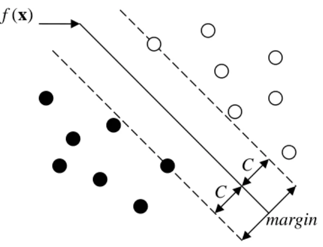
Figure 1: Separable case.

separated classes (see Figure 1). Since the classes are separable, we can find a function

First, consider two perfectly ( )

f x = ⋅ +w x b with y_j ⋅f(x_j)>0 for all j. Hence we can find the hyperplane that maximizes the margin between the training points for class {+1} and {-1}. The following optimization problem captures this concept.

, , 1 max C ( ) , 1, , . b j j subject to y b C j n = ⋅ + ≥ = w w w x … (8)

The band in Figure 1 is units away from the hyperplane on either side, hence 2 units

and defining

C C

wide. We can rephrase this problem more conveniently by dropping the norm constraint on

w C=1 w . , min ( ) 1, 1, b j j subject to y ⋅ + ≥b j= n w w w x …, . (9) (Recall that w x⋅ +b

w is the distance from to the hyperplane.) The expression in (9) is

the usual way of writing the support vector criterion.

x C C margin ( ) f x

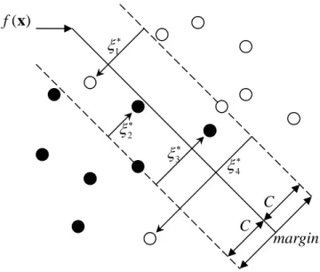
Figure 2: Non-separable case.

Suppose now the classes overlap in feature space. One way to deal with the overlap is to still maximize C but allow for some points to be on the wrong side of the margin (see , Figure 2). Define the slack variables ξ =( ,ξ ξ_{1 2},…,ξ_n). We modify the constraint in (8) by:

, , 1 max ( ) (1 ), 1, b j j j C subject to y b C ξ j n = ⋅ + ≥ − = w w w x …, , (10)

where . The points labeled

1

0 for all , and n constant

j j _j j

ξ ≥

∑

in Figure 2 are on the

wrong side of their margin by an amount ξ∗_j =Cξ_j; points on the correct side have ξ_j = 0. Misclassifications occur when ξ_j > , hence by the constraint 1

1 constant

n j j=ξ ≤

∑

the total number of training misclassification. As in (8), we can rephrase (9) in the equivalent form , 1 min ( ) 1 , 1, . 0, constant b j j j n j _j j y b j subject to ξ ξ ₌ξ ⋅ + ≥ − = ⎧⎪ ⎨ ≥ ≤ ⎪⎩

∑

By the nature of the criterion (11), we see that points well inside their class boundary do not play a crucial role in shaping the boundary.

C C margin 2 ξ∗ 4 ξ∗ 3 ξ∗ 1 ξ∗ ( ) f x

The problem (11) can be solved using Lagrange multipliers with the following equivalent form: 2 , 1 1 min 2 0, ( ) 1 , 1, , , n j b j j j j j subject to y b j n γ ξ ξ ξ = + ≥ ⋅ + ≥ − =

∑

where γ replaces the constant in (11); the separable case corresponds to γ = ∞ . The generalized Lagrange (primal) function is

2 1 (1 ) n n p j j j L 1 1 1 ( ) ( ), 2 n j j j j j j j y b γ ξ α ⎡ ξ = w +

∑

∑

∑

j j j j= 14) ( 1 , n y α =

∑

∑

α β ξ ≥ ∀ Classical Lagrangian duality enables as well as the positivity constraints

the primal problem to be transforme roblem, which is easier to solve. By substituting (14)-(16) into (13), we obtain the Lagrangian dual objective function

d to its dual p ' ' ' 1 , n n n T 1 2 1 ' 1 D j j j j j j j L =

∑

∑∑

which gives a lower bound on the objective function (12) for any feasible point. We maximize

D L subject to 0≤α_j ≤ and γ 0. n jyj α 1 j= =

∑

(1

j

α ⎡

con e the cons

j yj j b j ξ ) ( )⎤ 0, , − − w x⋅ + _⎦= ∀ (18) ⎣ ( ) 0, , j j j β −ξ = ∀ (19) (1−ξ_j)−y_j(w x⋅ _j+ ≤ ∀b) 0, j, (20)

Together these equations (14)-(20) uniquely characterize the s

(14), the solution of is of the form

21)

with nonzero coefficients

olution to the primal and dual problem. From w 1 ˆ ˆ _{j j j} j y α = =

∑

α only for those ob

lutions for n

, the decision function can be written as

servations for which the constraints in (20)

are exactly met (due to (18)). These observations are called support vectors, since wˆ is represented in terms of them alone. From (18) we can see that any of these margin points

(0<α ξˆ_j, ˆ_j = ) can be used to solve for 0 bˆ, and we typically use an average of all the so umerical stability.

Given the solutions wˆ and bˆ

[

]

ˆ

ˆ_{( ) ( ) ˆ .}

D x =sign f⎡_⎣ x ⎤_⎦=sign w x⋅ +b (22) The tuning parameter of this procedure is γ. In general, the classification problem is fairly insensitive to γ. We let γ = ∞ which corresponds to the linear separable case, in this , study.

3.3 The Proposed Gene Selection Scheme

lection scheme. First, in order to avoid selec

It takes four steps to implement our gene se

ting irrelevant genes after clustering and to reduce the computational cost, we filter out genes with no or little effect to classification according to a ranking criterion, say, the absolute values of (2), (3), or (4). However, it is rather difficult to have a general principle concerning the amount of genes we should filter for each application. For convenience, we filter out 90% of genes. It seems a plausible number when we start with thousands of genes. Second, we cluster the rest 10% genes via K-means algorithm for a given number of clusters, K to , avoid redundancy. Third, a preliminary selection procedure is performed by selecting some

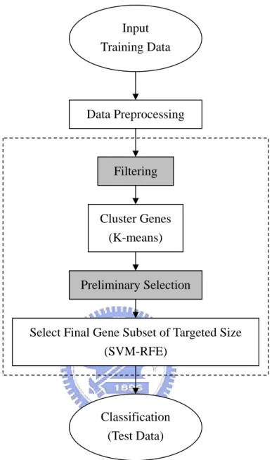
informative genes from each cluster according to the same ranking criterion used in the first step. Tens of genes are often considered to build a predictor in the literature. Golub et al. (1999) selected 50 genes for leukemia data according to (2). Dudoit et al. (2002) selected 50 genes with the largest values of (4) for the lymphoma dataset, 40 genes for the leukemia dataset, and 30 genes for the NCI60 dataset. Nevertheless, some datasets can be well separated by merely several genes, e.g., leukemia data (Xiong et al. (2001); Guyon et al. (2002)). Here, candidate genes, ranging from 50 to 100 in number, are selected proportionally from each cluster. Fourth, SVM-RFE, in which RFE is performed based on SVM classifier, is used to decide one final gene subset of targeted size from the candidate genes selected by the preceding step. The complete process of data analysis is schemed in Figure 3. Steps 1 and 3 require a ranking criterion. In this study, we consider the following three ranking criteria: absolute values of (2), (3), and (4) and call them ranking method (2), (3), (4), respectively. We remark that data preprocessing is still an open issue. In this study, we only standardize each gene such that the mean is 0 and standard deviation is 1 across subjects here.

Figure 3: Flowchart of data analysis. The dashed-line box is our gene selection scheme. The steps marked with gray background are implemented with a ranking criterion.

Filtering

Cluster Genes (K-means)

Preliminary Selection

Select Final Gene Subset of Targeted Size (SVM-RFE) Classification (Test Data) Data Preprocessing Input Training Data

4. Data Analysis

We apply the proposed gene selection scheme to three popular microarray datasets in the literature, the leukemia data (Golub et al., 1999), colon cancer data (Alon et al., 1999), and breast cancer data (Hedenfalk et al., 2001). Combinations of each of the three ranking methods described before with RFE (Guyon et al., 2002) are considered in this study. For convenience, we call these combinations Scheme Ⅰ, Ⅱ, and Ⅲ, respectively. Furthermore, we compare our gene selection scheme with the corresponding ranking method and the RFE.

In the absence of test data in the colon cancer data and breast cancer data, leave-one-out cross validation (LOOCV) is adopted to evaluate the performance of the methods in this study. More specifically, for each subject, remove it from the original dataset, train the rest of data to build a classifier, and then test the classifier on the removed subject. The three publicly available datasets have been processed in many different ways by analysts, including experimental design, normalization, outlier elimination, etc. Most of these preprocessing works were beyond our control, especially the variation removal between chips (subjects). Without transforming the data to attain the consistency, we merely standardize each gene of the training set such that the mean is 0 and standard deviation is 1 across subjects to ensure comparability with each other.

We filter out 90% of genes and cluster the rest genes into =1~30 clusters. In addition, we use the cumulative frequency plot of the values of each ranking criterion as an auxiliary to judge whether it is adequate to cluster only 10% of genes.

K

4.1 Leukemia Data

The gene expression levels of the leukemia data (Golub et al., 1999) were produced by

Affymetrix high-density oligonucleotide microarrays. The data contain two subsets: a training data set used to select genes and create the classifier, and an independent test data set used to

assess the performance of the classifier. The training set consists of 38 bone marrow subjects (27 ALL (acute lymphoblastic leukemia), 11 AML (acute myeloid leukemia)) obtained from acute leukemia patients at the time of diagnosis. The test set has 34 leukemia subjects (20 ALL, 14 AML), including 24 bone marrow and 10 peripheral blood subjects, and data are from different reference laboratories that used different subject preparation protocols. Each dataset contains 7,129 genes. The problem of interest is to distinguish between two types of leukemia, ALL and AML. We pool two datasets, training set and test set, together and implement LOOCV on it. The following are some results:

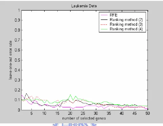
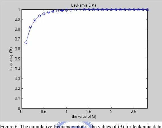
● Figure 4 displays the leave-one-out error rates of RFE and the three ranking methods. RFE is obviously better than all three ranking methods when the number of selected genes is small, and the results of all three ranking methods are similar. ● Figures 5-7 give, respectively, the cumulative frequency plots of the three different

ranking values of all subjects. It is noted that filtering out 90% of genes seems plausible because of those 90% genes have smaller ranking values relatively. ● After clustering, we select about 10% genes from each cluster to form a set of

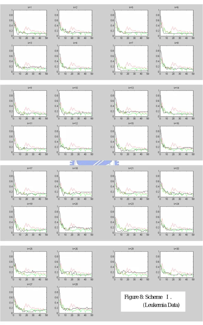
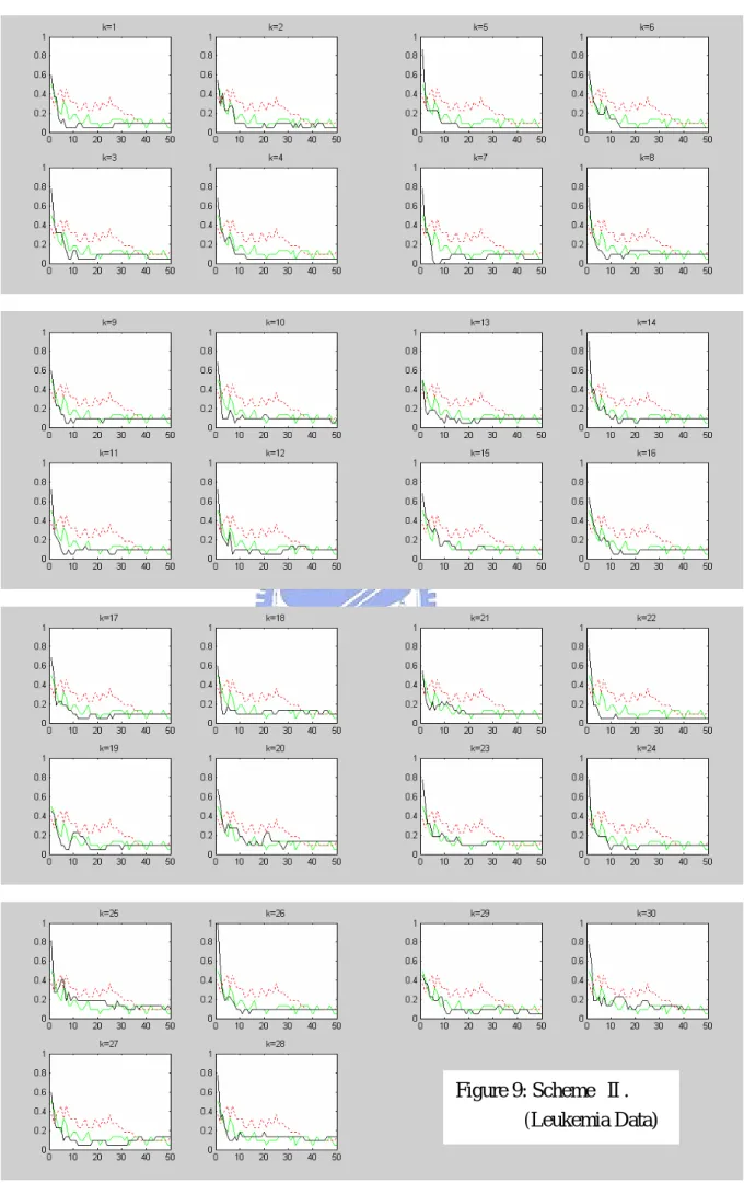
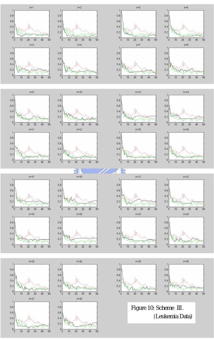
candidate genes of size around 70. SVM-RFE is applied to this set. Figures 8-10 show the leave-one-out error rate only for 1-50 selected genes, for each in a subplot, of schemes Ⅰ-Ⅲ (solid line), respectively. In addition to the results of our gene selection scheme, we also plot the leave-one-out error rates of RFE (undertone solid line) and the corresponding ranking method (dashed line) in each subplot.

K

We note that when the number of genes reduces to 1, the error rate is always the largest in our three schemes. However, our schemes indeed perform better than the three ranking methods. Among three schemes, scheme Ⅱ performs the best and almost as good as RFE.

4.2 Colon Cancer Data

oligonucleotide arrays. After pre-processing, the data set contains the expression of the 2,000 genes with highest minimal intensity across the 62 tissues. The 62 tissues include 22 normal and 40 colon cancer tissues.

● Figure 11 displays the leave-one-out error rates of RFE and the three ranking methods. Although all curves are fairly flat about the value 0.2, it still can be seen that all three ranking methods all perform better than RFE.

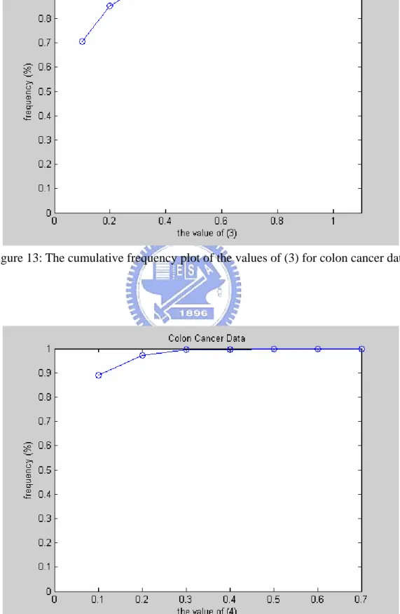
● Figures 12-14 give, respectively, the cumulative frequency plots of the three different ranking values of all subjects. These ranking values are obviously smaller than that of the leukemia data. Filtering out 90% of genes also seems acceptable. However, in order to avoid leaving out informative genes, we take 300 top-ranked genes for clustering in the three schemes.

● After that, we select 20% genes from each cluster such that the size of the gene set will be around 60 in number. The leave-one-out error rates of schemes Ⅰ-Ⅲ (solid line) on this subset for different are plotted in Figures 15-17, respectively. Each subplot accompanies the results of RFE (undertone solid line) and the corresponding ranking method (dashed line).

K

The curve of our method for each is still flat but slightly higher than the other two methods for all three schemes. This is probably due to that ranking methods in themselves perform better than RFE. And it is notable that all curves are fairly flat in the number of selected genes for this dataset, that is, we can not get better result even if we increase the number of selected genes.

K

4.3 Breast Cancer Data

The breast cancer data (Hedenfalk et al., 2001) were produced by cDNA mircorarray

in this dataset. Each tissue corresponds to one of three mutations of breast cancer, that is, BRCA1, BRCA2, and Sporadic. There are 7 BRCA1, 8 BRCA2, and 7 Sporadic. We let BRCA1 as one class and pool BRCA2 and Sporadic as another class.

● Figure 18 displays the leave-one-out error rates of RFE and the three ranking methods. We observe that RFE is better than the ranking methods, especially when the number of the selected genes is less than 20.

● Figures 19-21 give, respectively, the cumulative frequency plots of the three different ranking values of all subjects. Filtering out 90% of genes is still acceptable.

● After clustering, we select 20% genes from each cluster so that the size of the gene set is around 60 in number. Apply SVM-RFE to this gene set. Figures 22-24 show the plots of leave-one-out error rate for schemes Ⅰ-Ⅲ (solid line), respectively. Each subplot accompanies the results of RFE (undertone solid line) and the corresponding ranking method (dashed line).

It is obvious that our method has a smaller error rate than that of the corresponding ranking method when the number of genes is less than 20 for all three schemes. However, our three schemes perform poorly when the number of genes is larger than 20. Scheme Ⅲ (Figure 24) performs slightly better than others (Figures 22-23).

We repeat the experiment but select around 100 candidate genes from clusters. SVM-RFE is applied to this new subset, and the results are shown in Figures 25-27. These results are better than the preceding case. When the number of genes is larger than 20, scheme Ⅲ (Figure 27) performs better than three ranking methods. When the number of the selected genes is between 15 and 20, our schemes always perform better than RFE.

5. Conclusions and Future Research

We propose a gene selection scheme by combining two conventional gene selection methods, ranking methods and RFE, in this study. Ranking methods are fast in computation but might select highly correlated genes that give rise to redundancy to the classification problem, while RFE can select a set of non-redundant genes but requires extensive computation. The K-means clustering algorithm is used to reduce redundancy that arises from the ranking criterion. Before clustering, we filter out 90% of genes to avoid selecting irrelevant genes. A set of candidate genes are selected with the same proportion from each cluster. After that, SVM-RFE is applied to this subset to get a final gene subset of an expected size. The proposed gene selection scheme is applied to three popular microarray data sets. In general, ranking methods usually perform poorly when compared with RFE. Under this situation, our method can reduce error rate effectively when the size of gene subset is less than 20 and but may not always be as good as RFE. Nevertheless, our method is faster than RFE in computation. There are some issues not addressed in this study:

● The choice of K

We use =1~30 in our experiments. Our combined method does not perform very well when is small or fairly large, so =5~20 is suggested. We also conduct a preliminary study on the choice of Two criteria are used to choose the correct number of clusters, but they always choose the smallest The first criterion was proposed by Calinski and Harabasz (1974):

K K K . K . K ( ) /( 1) max ( ), ( ) , ( ) /( ) k B k k CH k CH k W k n k − = −

where B k and ( ) are the between and within cluster sums of squares with clusters, respectively. is not defined. Milligan and Cooper (1985) conducted a comprehensive simulation comparison of 30 different procedures.

( )

W k

gap statistic proposed by Tibshirani et al. (2001):

*

max _n( ), _n( ) _n(log( _k)) log( ).

k Gap k Gap k =E W − Wk

One direction for future work is to try other clustering methods, e.g., model based clustering, then AIC or BIC criterion can be used to choose K.

● Threshold of filtering

In this study, we filter out 90% of genes before clustering. And the cumulative frequency plot of the values of the ranking criterion is used as an auxiliary to see if 90% filtering is acceptable. This is an acceptable number from the results of data analysis. Other explicit methods can also be tried.

● How to select candidate genes from each cluster?

Only the size of each cluster plays a part in selecting candidate genes in our study. However, it is possible that selecting only one genes from a cluster with fewer genes when is large. In order to avoid information loss, we suggest that selecting 2~3 genes from each cluster at least. In view of the results of the breast cancer data, we also suggest that the number of genes in the final step of our scheme, SVM-RFE, is 100 for general cases.

K

● How many genes should be selected in the end?

This question can only be answered by biologists. They can make a decision according to how much time they can invest in examining these genes further and how much loss they can risk.

Guyon et al. (2002) observed in real experiments that a slight change in the feature set

often results in a completely different RFE ordering. Therefore, other combinations of filters and wrappers can be tried. In addition, the datasets used in this study were produced several years ago and microarray techniques are in progress. We hope that the proposed method can be applied to some new datasets.

References

[1] Alon, U., Barkai, N., Notterman, D. A., Gish, K., Ybarra, S., Mack, D., and Levine, A. J. (1999). “Broad patterns of gene expression revealed by clustering analysis of tumor and normal colon tissues probed by oligonucleotide arrays.” Proceedings of the National Academy of Sciences of the United States of America, 96, 6745-6750, Cell Biology. The

dataset is available on-line at http://www.weizmann.ac.il/mcb/ UriAlon/.

[2] Calinski, R. B. and Harabasz, J. (1974). “A dendrite method for cluster analysis,”

Communications in statistics, 3, 1-27.

[3] Ding, C. and Peng, H. (2003). “Minimum redundancy feature selection from microarray gene expression data.” Proc. 2nd IEEE Computational Systems Bioinformatics Conference (CSB 2003), 523-528.

[4] Doduit, S., Fridlyand, J., and Speed, T. P. (2002). “Comparison of discrimination methods for the classification of tumors using gene expression data.” Journal of the American Statistical Association, 97, 77-87.

[5] Furey, T. S., Cristianini, N., Duffy, N., Bednarski, D. W., Schummer, M., and Haussler, D. (2000). “Support vector machine classification and validation of cancer tissue samples using microarray expression data.” Bioinformatics, 16, 906-914.

[6] Golub, T. R., Slonim, D. K., Tamayo, P., Huard, C., Gaasenbeek, M., Mesirov, J. P., Coller, H., Loh, M. L., Downing, J. R., Caligiuri, M. A., Bloomfield, C. D., and Lander, E. S. (1999). “Molecular classification of cancer: class discovery and class prediction by gene expression monitoring.” Science, 286, 531-537. The dataset is available on-line at

http://www.genome.wi.mit.edu/MPR/data_set_ALL_AML.html.

[7] Guyon, I., Weston, J., Barnhill, S., and Vapnik, V. (2002). “Gene selection for cancer classification using support vector machines.” Machine Learning, 46, 389-422.

data mining, inference, and prediction. Springer-Verlag, New Work.

[9] Hedenfalk, I., Duggan, D., Chen, Y., Radmacher, M., Bittner, M., Simon, R., Meltzer, P., Gusterson, B., Esteller, M., Kallioniemi, O.-P., Wilfond, B., Borg, Å., and Trent, J. (2001). “Gene-expression profiles in hereditary breast cancer.” The New England Journal of Medicine, 344, 539-548. The dataset is available on-line at

http://research.nhgri.nih.gov/microarray/NEJM_Supplement/.

[10] Jaeger, J., Sengupta, R., and Ruzzo, W. L. (2003). “Improved gene selection for classification of microarrays.” Appeared in Pacific Symposium on Biocomputing, 2003,

53-64.

[11] Milligan, G. W. and Cooper, M. C. (1985). “An examination of procedures for determining the number of clusters in a data set.” Psychometrika, 50, 159-179.

[12] Nadon, R. and Shoemaker, J. (2002). “Statistical issues with microarrays: processing and analysis.” Trends in Genetics, 18, 265-271.

[13] Pavlidis, P., Weston, J., Cahi, J., and Grundy, W. N. (2000). “Gene functional classification from heterogeneous data.” Submitted for publication.

[14] Sebastiani, P., Gussoni, E., Kohane, I. S., and Ramoni, M. F. (2003). “Statistical challenges in functional genomics.” Statistical Science, 18, 33-70.

[15] Tibshirani, R., Walther, G., and Hastie, T. (2001). “Estimating the number of clusters in a data set via the gap statistic.” Journal of the Royal Statistical Society – Series B Statistical Methodology, 63, 411-423.

[16] Tseng G. C. and Wong W. H. (2003). “Tight clustering: a resampling-based approach for identifying stable and tight patterns in data.” Biometrics. (To Appear).

[17] Xiong, M., Li, W., Zhao, J., Jin, L., and Boerwinkle, E. (2001). “Feature (Gene) selection in gene expression-based tumor classification.” Molecular Genetics and Metabolism, 73,

Figures

Figure 4: The leave-one-out error rates of RFE and the three ranking methods for leukemia data.

Figure 6: The cumulative frequency plot of the values of (3) for leukemia data.

Figure 8: Scheme Ⅰ. (Leukemia Data)

Figure 9: Scheme Ⅱ. (Leukemia Data)

Figure 10: Scheme Ⅲ. (Leukemia Data)

Figure 11: The leave-one-out error rate of RFE and the three ranking methods for colon cancer data.

Figure 13: The cumulative frequency plot of the values of (3) for colon cancer data.

Figure 15: Scheme Ⅰ. (Colon Cancer Data)

Figure 16: Scheme Ⅱ. (Colon Cancer Data)

Figure 17: Scheme Ⅲ. (Colon Cancer Data)

Figure 18: The leave-one-out error rate of RFE and the three ranking methods for breast cancer data.

Figure 20: The cumulative frequency plot of the values of (3) for breast cancer data.

Figure 22: Scheme Ⅰ. (Breast Cancer Data)

Figure 23: Scheme Ⅱ. (Breast Cancer Data)

Figure 24: Scheme Ⅲ. (Breast Cancer Data)

Figure 25: Scheme Ⅰ with 100 genes (Breast Cancer Data)

Figure 26: Scheme Ⅱ with 100 genes (Breast Cancer Data)

Figure 27: Scheme Ⅲ with 100 genes (Breast Cancer Data)