Mining Closed Sequential Patterns with Time Constraints

全文

(1)Mining Closed Sequential Patterns with Time Constraints. 1. Ming-Yen Lin1, Sue-Chen Hsueh2, and Chia-Wen Chang1 Department of Information Engineering and Computer Science, Feng Chia University, Taiwan 2 Department of Information Management, Chaoyang University of Technology, Taiwan [email protected], [email protected], [email protected] ABSTRACT. The mining of closed sequential patterns has attracted researchers for its capability of using compact results to preserving the same expressive power as traditional mining. Many studies have shown that constraints are essential for applications of sequential patterns. However, time constraints have not been incorporated into closed sequence mining yet. Therefore, we propose an algorithm called CTSP for closed sequential pattern mining with time constraints. CTSP loads the database into memory and constructs time-indexes to facilitate both pattern mining and closure checking, within the pattern-growth framework. The index sets are utilized to efficiently mine the patterns without generating any candidate or sub-database. The bidirectional closure checking strategy further speeds up the mining. The comprehensive experiments with both synthetic and real datasets show that CTSP efficiently mines closed sequential patterns satisfying the time constraints, and has good linear scalability with respect to the database size.. 1: INTRODUCTION Sequential pattern mining [1, 3, 6, 15], which discovers frequent sub-sequences in a sequence database, is becoming an active research topic for its wide applications including customer behavior analysis, web usage mining, DNA sequence analysis, etc. The discovered sequential patterns disclose not only the frequent items or events occurred together, but also the sequences of frequently appeared item-sets or events. Many studies have shown that specifying constraints may increase the accuracy of mining results in practice. Various constraints, such as item, length, super-pattern, duration, and gap, can be specified to find more desirable patterns. Some constraints can be handled by a post-processing on the result of mining without constraints. However, time constraints affect the support computation of patterns so that they cannot be handled without adapting time attributes into the mining algorithms. The issue of mining sequential patterns with time constraints was first addressed in [2]. Three time constraints including minimum gap, maximum gap and sliding time-window are specified to enhance the semantics of sequence discovery. For example, in a. retail application, a discovered sequential pattern may be <(TV)(Audio, Jukebox)> which means most customers could buy Audio and Jukebox after purchasing TV. However, if the time gap between two adjacent transactions in a pattern is long, such as over one year, the pattern could be useless for sales promotion. Specifying maximum gap helps to filter out such patterns. Moreover, if three days is indispensable for the supply of the stock and the time gap between two adjacent transactions in a pattern is less than two days, the pattern is unhelpful to replenish stocks in time. Minimum gap can be used so that the unhelpful patterns would not be displayed. Additionally, a consumer may forget to buy some goods in a transaction and buy them in the subsequent transaction within two days. A sliding window of two days may allow the two transactions to be handled (combined) as one. For instance, a data sequence <1(TV)7(Audio)9(Jukebox)> can support pattern <(TV)(Audio, Jukebox)>. Therefore, adding time constraints for better mining results is an important problem. In addition to time-constrained sequential pattern mining [2, 9, 10, 11, 19], the issue of mining sequential patterns has been extended. Various topics such as maximal sequential pattern mining, closed sequential pattern mining [5, 16, 17], top-k sequential pattern mining [14] and so on are studied. A sequential pattern is maximal if it is not a subsequence of another frequent sequence. It is closed if no any frequent super-sequence has the same support. For example, if sequential patterns with supports including <(a)>:3, <(c)>:3, <(e)>:2, <(a)(c)>:2, <(a)(e)>:2, (c, e):2, <(a)(c, e)>:2 are found, the closed patterns are <(a)>:3, <(c)>:3, <(a)(c, e)>:2, and the maximal pattern is <(a)(c, e)>:2 only. Although the closed patterns are more compact than the complete set of patterns, the same amount of information can be derived. For instance, the support of <(a)(c)>, being 2, can be derived from <(a)(c, e)>. Many algorithms [3, 4, 8, 18] have been proposed to deal with the problem of mining sequential patterns. In general, these algorithms can be categorized into Apriori-like framework such as GSP [2] and SPADE [18], and pattern-growth framework such as PrefixSpan [12]. Although algorithms such as prefix-growth [13], DELISP [9], and cSPADE [19] may handle time constraints, they generally provide the complete set of time-constrained patterns, rather than the compact closed patterns. Algorithms CloSpan [17] and BIDE [16]. - 346 -.

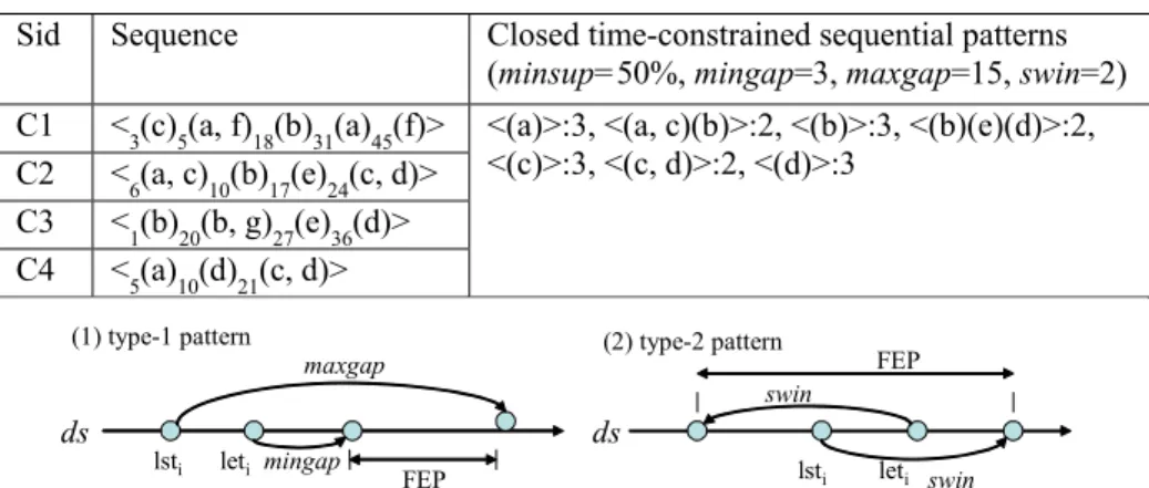
(2) successfully mines closed sequential patterns. However, the time constraint is yet to be incorporated. To the best of our knowledge, no algorithm has been presented to solve the problem of mining closed sequential patterns with time constraints. Therefore, we propose an algorithm called CTSP (Closed Time-constrained Sequential Pattern mining) for mining closed sequential patterns with minimum gap, maximum gap, and sliding window constraints. Moreover, we define the closure of time-constrained patterns by contiguous sub/supersequences so that true time-constrained patterns with correct supports can be derived. CTSP utilizes the memory for efficient mining. Time-indexes are constructed in CTSP to facilitate both pattern mining and closure checking, within the pattern-growth framework. The closure checking is performed bi-directionally to speed up the mining. The extensive and comprehensive experiments with both synthetic and real datasets show that CTSP efficiently mines closed sequential patterns satisfying the time constraints, and has good linear scalability with respect to the database size.. 2: Problem Statement Let Ψ = {α1, α2, …, αr} be a set of literals, called items. An itemset I = (β1, β2, …, βq) is a nonempty set of q items such that I ⊆ Ψ. A sequence s, denoted by <e1e2…ew>, is an ordered list of w elements where each element ei is an itemset. Without loss of generality, we assume the items in an element are in lexicographic order. The length of a sequence s, written as |s|, is the total number of items in all the elements in s. Sequence s is a k-sequence if |s| = k. The sequence database DB contains |DB| data sequences. A data sequence ds has a unique identifier sid and is represented by <t1e1’ t2e2’ … tnen’>, where element ei’ occurred at time ti , t1 < t2 < ...< tn. A sequence s in the sequence database DB is a time-constrained sequential pattern (abbreviated as time-pattern) if s.sup ≥ minsup, where s.sup is the support of the sequence s and minsup is the user specified minimum support threshold. The support of sequence s is the number of data sequences containing s divided by |DB|. Note that the support calculation has to satisfy three time-constraints maxgap (maximum gap), mingap (minimum gap), and swin (sliding window). A data sequence ds = <t1e1’ t2e2’… tnen’> contains a sequence s = <e1e2…ew> if there exist integers l1, u1, l2, u2, …, lw, uw and 1 ≤ l1 ≤ u1 < l2 ≤ u2 < …< lw ≤ uw ≤ n such that the four conditions hold: (1) ei ⊆(el ’∪…∪. without time constraints is a special case by setting mingap = 1, maxgap = ∞, swin = 0. A sequence s is closed if no contiguous supersequence ssup with the same support exists. Given a sequence s = <e1e2…ew> and a subsequence ssub of s, ssub is a contiguous subsequence of s if ssub can be obtained by any one of following ways: (1) dropping an item from either e1 or ew (2) dropping an item from element ei (1 ≤ i ≤ w) which has least two items (3) ssub is a contiguous subsequence of ssub’, and ssub’ is a contiguous subsequence of s. Additionally, s is called a contiguous supersequence of ssub. A sequence s is a closed time-constrained sequential pattern, abbreviated as closed time-pattern, if it is a time-pattern and is closed. The mining aims to discover the set of all closed time-patterns. For example, given a sequence DB of four data sequences with their sids in Table 1, the rightmost column shows the closed time-patterns for constraints mingap = 3, maxgap = 15, swin = 2, and minsup = 50%. In Table 1, data sequence C4 <5(a)10(d)21(c, d)> has three itemsets occurring at time 5, 10, 21, respectively. The third itemset of C4 has two items c and d. Sequences <(a,c)(b)> and <(b)(e)(d)> are both 3-sequences. The sequence <(a,c)(b)> is contained in data sequences C1 <3(c)5(a, f)18(b)31(a)45(f)> because element (a,c) can be contained in the transaction combining 3(c) and 5(a, f) for 5-3≤ 2 (swin). Meanwhile, the mingap and maxgap constraints are satisfied for 18-5 ≥ 3 and 18-3 ≤ 15. Similarly, <(a,c)(b)> is contained in C2. The support of <(a,c)(b)> is 2/4 and it is a time-pattern for minsup = 50%. <(a,c)(b)> is also a closed time-pattern since it has no contiguous supersequence with the same support. <(c)(b)> is a time-pattern for <(c)(b)>.sup = 2/4 but not closed for its contiguous supersequence <(a,c)(b)> having the same support. The notion of contiguous subsequence (supersequence) is introduced to guarantee the correctness and completeness of closed time-patterns. The subsequence of a (closed) time-pattern is not necessary a (closed) time-pattern if the contiguous relationship is not hold. For example, though <(b)(d)> is the subsequence of <(b)(e)(d)>, time-pattern <(b)(e)(d)> does not imply that <(b)(d)> is also a time-pattern since <(b)(d)> fails the maxgap constraint in C3. However, <(b)(e)(d)> of support 2/4 ensures that its contiguous subsequences, such as <(b)(e)> and <(e)(d)>, are also time-patterns with support 2/4. Such a definition enables the close time-patterns to have the same expressive power with more compact patterns.. i. eu ’), 1 ≤ i ≤ w (2) tu - tl ≤ swin, 1 ≤ i ≤ w (3) tu - tl ≤ i i i i i-1 maxgap, 2 ≤ i ≤ w (4) tl - tu ≥ mingap, 2 ≤ i ≤ w.. 3: CTSP: Closed Time-constrained Sequential Pattern mining. Assume that tj, mingap, maxgap, swin are all positive integers, maxgap ≥ mingap ≥ 1. When mingap is the same as maxgap, the time constraint is additionally called exact gap. Common sequential pattern mining. The algorithm we proposed for mining closed time-patterns is called CTSP. CTSP uses the pattern-growth methodology [8, 12, 13] to discover the desired patterns and the bi-directional strategy, similar to. i. i-1. - 347 -.

(3) BIDE [16], to check the closure property. The algorithm is described as follows. Definition 1 (frequent item) An item x is called a frequent item in DB if <(x)>.sup ≥ minsup. Definition 2: (type-1 pattern, type-2 pattern, stem, prefix) Given a frequent pattern P and a frequent item x in DB, P’ is a type-1 pattern if it can be formed by adding an itemset of the single item x after the last element of P, and a type-2 pattern if formed by appending x to the last element of P. For type-2 pattern, the lexicographic order of x must be larger than all items in the element. The item x is called the stem of the new frequent pattern P’. The prefix pattern (abbreviated as prefix) of P’ is P. For example, <(a)(b)> is a type-1 pattern by adding (b) after <(a)>, and <(a, c)> is a type-2 pattern by appending (c) to <(a)>. Here, (b) and (c) are the stems and <(a)> is the prefix pattern. Definition 3: (last-start time, last-end time, time-index) Let the last element of a frequent pattern P be LE. If ds contains P by having LE ⊆ eγ ∪eγ+1∪ …∪eω, where eγ,…, eω are elements in ds, the occurring time tγ and tω for itemsets eγ and eω are named, respectively, last-start time (abbreviated as lst) and last-end time (abbreviated as let) of P in ds. Every occurrence of the lst:let pair is collected altogether as [lst1:let1, lst2:let2,…, lstk:letk], lsti ≤ leti for 1 ≤ i ≤ k. Such a timestamp lists is called the time-index of P in ds. In addition to stems, items in the backward direction of a frequent pattern P, i.e. occurring before P, may be used to form P’ and speed up the mining process. For example, P = <(a)(b)> is contained in s = <2(e)6(a, c)10(b, d)18(a)> with time-index [6:10]. Stem (a) (timestamp 18) may extend P to a type-1 pattern <(a)(b)(a)> and stem (d) (timestamp 10) may extend P to a type-2 pattern <(a)(b, d)> in the forward direction. Considering the (a) in P, item (e) (timestamp 2) and item (c) (timestamp 6) can be used to form contiguous supersequences <(a, c)(b)> and <(e)(a)(b)>, respectively. The two non-stem items are found in the backward direction of P. Thus, we have the following definition. Definition 4: (extension item, extension period) Given a frequent pattern P contained in ds, a non-stem item α in ds is called an extension item (abbreviated as EI) if it can be used in extending P to form a contiguous supersequence P’ satisfying the time constraints. The time periods within which α exists is called extension period (abbreviated as EP). The time period is referred to as backward extension period (abbreviated as BEP) and the item is called backward extension item (abbreviated as BEI). For convenience, we refer to the time period within which stems exist as forward extension period (abbreviated as FEP). Lemma 1: Given a time-index of frequent pattern P in ds [lst1:let1, lst2:let2,…, lstk:letk], the FEP satisfies either one of the following conditions: (1) ∃ i, 1 ≤ i ≤ k, leti+mingap ≤ FEP ≤ lsti+maxgap (2) ∃ i, 1 ≤ i ≤ k, leti-swin ≤ FEP ≤ lsti+swin. Fig. 1 illustrates Lemma 1.. Definition 5: (timeline) Given a frequent pattern P = <e1…er…ew> in ds. If e1 ⊆ est1∪…∪eet1, …, er ⊆ estr∪…∪eetr, …, and ew ⊆ estw∪…∪eetw, where est1, …, estw, eet1, …, eetw are elements in ds, the list of timestamps [st1:et1, …, str:etr, …, stw:etw] where str ≤ letr for 1≤ r ≤ w is called the timeline of P in ds. Note that the ds may have several timelines of P. For example, P = <(a)(d)(e)> can be found in ds = <5(b)9(a)13(d)14(c)16(e)19(e)> with timeline [9:9, 13:13, 16:16] and timeline [9:9, 13:13, 19:19]. The two timelines, implemented as linked lists, are shown in Fig. 2. Lemma 2: Given a frequent pattern P = <e1…er…ew> contained in ds. For each timeline [st1:et1,…,str;etr,…,stw:etw] of P in ds, the BEP satisfies either one of the following conditions: (1) et1-maxgap ≤ BEP ≤ st1-mingap (2) ∃ i, 1 ≤ i ≤ w, eti-swin ≤ BEP ≤ sti or eti ≤ BEP ≤ sti+swin. Lemma 2 is illustrated in Fig. 3. Forming a type-2 pattern with the potential stems using Lemma 1 can be pruned in advance if the stem is lexicographically smaller than the items of the last element in P. Moreover, the time periods are checked on not violating the minimum/maximum gap constraints between adjacent elements when a type-2 pattern is formed. Lemma 3: Given a frequent pattern P, if a stem to be used in extending P to P’ is found in every data sequence containing P, then P is not a closed time-pattern. Lemma 4: Given a frequent pattern P, if a BEI to be used in extending P to P’ is found in every data sequence containing P, then P is not a closed time-pattern. Fig. 4 outlines the CTSP Algorithm, which mines patterns within the pattern-growth framework. The techniques used are similar to the pseudo projection version of Prefixspan algorithm [12] and bi-direction closure checking in BIDE algorithm [16], while it can handle constraints minimum/maximum gaps and sliding time-window. Assume that the DB can fit into the main memory, CTSP first loads DB into memory (as MDB) and scans MDB once to find all frequent items. With respect to each frequent item, CTSP then constructs a time-index set for the 1-sequence item and recursively forms time-patterns of longer length. The time-index set is a set of (data-sequence pointer, time-index) pairs. Only those data sequences containing that item would be included. The time-index indicates the list of lst:let pairs as described in Definition 3. In Fig. 4, CMine (P, P-Tidx) mines type-1 patterns and type-2 patterns having prefix P by effectively locating FEPs with Lemma 1. The P-Tidx is the time-index set for P. CTSP thus never search the data sequences irrelevant to P. Moreover, the FEPs ensure that CTSP locates and counts the effective stems which can form valid patterns, rather than the whole set of items in the data sequence. Furthermore, CTSP adopts forward and backward closure checking to examine the closure of prefix P. The supports of potential stems and. - 348 -.

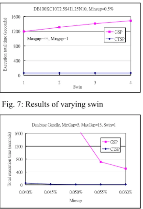
(4) BEIs are handled by forward closure checking and backward closure checking, respectively. If neither stem nor BEI has the same support as P, then P is a desired closed time-pattern. Recursively, for a newly formed type-1 pattern or type-2 pattern P’, its time-index set P’-Tidx is constructed and CMine(P’, P’-Tidx) is invoked. By pushing time attributes deeply into the mining process, CTSP efficiently discovers the desired patterns. If the database is too large to fit into memory, a projected scheme is applied. The database will be projected to small sub-databases, based on the frequent 1-sequences. Each sub-database then can be mined by the CTSP. A similar technique has been adopted in the Par-CSP algorithm [5]. Therefore, CTSP can mine databases, even when the size of the database is larger than that of main memory.. respectively. The number of closed patterns decreases as mingap increases or maxgap decreases. The gap constraints restrict more patterns so that the running time is decreased. The swin relaxes the constraint and allows more patterns to appear so that total execution time is increased. The result of varying minsup is shown in Fig. 8. The results of mining real dataset Gazelle (from KDD Cup 2000 [7]) are displayed in Fig. 9. The mingap, maxgap and sliding window are set as 3, 15 and 1, respectively. The Gazelle dataset has 29369 data sequences and 386 distinct items. The maximum sequence length and maximum session size are 628 and 267, respectively. CTSP is about 5 times faster than GSP for minsup = 0.06%. The result of scaling up the database size, from 100k to 1000k, in Fig. 10 indicates that CTSP has good linear scalability.. 4: Experimental Results. 5: Conclusion. Extensive experiments were performed on both synthetic and real datasets to assess the performance of the CTSP algorithm. Algorithm GSP, which mines all time-constrained sequential patterns without closure checking, was used to compare with CTSP. All experiments were performed on an AMD 2800+ PC with 1GB memory running the Windows XP. Here, we describe the result of dataset C10-T2.5-S4-I1.25 having 100000 data sequences (|DB| = 100k), with Ns=5000, NI=25000 and N=10000. The detailed parameters are addressed in [1]. The results of varying |C|, |T|, |S|, and |I| were consistent. CTSP outperforms GSP in all the experiments. Figures 5, 6 and 7 show the results of varying mingap, maxgap and sliding window constraints,. In this paper, we have presented an efficient algorithm called CTSP for mining closed sequential patterns with minimum/maximum gap and sliding window constraints. CTSP uses memory-indexes and the time constraints to shrinks the search-space effectively within the pattern-growth framework. The closure checking is bi-directionally performed. The experimental results show that CTSP has good performance with gap constraints, both for synthetic and real datasets.. Acknowledgements This work was supported partially by the National Science Council, Taiwan under grant NSC95-2221-E-035-114.. Table 1. Example sequence database (DB) and the closed time-constrained sequential patterns. Sid. Sequence. Closed time-constrained sequential patterns (minsup=50%, mingap=3, maxgap=15, swin=2). C1 C2 C3 C4. <3(c)5(a, f)18(b)31(a)45(f)> <6(a, c)10(b)17(e)24(c, d)> <1(b)20(b, g)27(e)36(d)> <5(a)10(d)21(c, d)>. <(a)>:3, <(a, c)(b)>:2, <(b)>:3, <(b)(e)(d)>:2, <(c)>:3, <(c, d)>:2, <(d)>:3. (1) type-1 pattern. (2) type-2 pattern. maxgap. FEP. swin. ds. lsti. leti mingap. ds lsti. FEP. leti swin. Fig. 1: The forward extension period for (a) type-1 pattern and (b) type-2 pattern (a). (d). (e). [9:9]. [13:13]. [16:16] (e) [19:19]. Fig. 2: The timelines of <(a)(d)(e)> in <5(b)9(a)13(d)14(c)16(e)19(e)>. - 349 -.

(5) (a) contiguous supersequence extension (type-1) maxgap. ds BEP mingap (b) contiguous supersequence extension (type-2) swin. ds. swin. st1. swin. et1. BEP. st1 swin. et1 swin. swin. str etr. stw etw. BEP. BEP. Fig. 3: Two types of backward extension period in extending a contiguous supersequence Algorithm: CTSP Input: DB (a sequence database), minsup (minimum support), mingap (minimum gap), maxgap (maximum gap), swin (sliding time-window). Output: the set of all closed time-constrained sequential patterns 1. load DB into memory (as MDB) and scan MDB once to find all frequent items. 2. for each frequent item x, (1) form the sequential pattern P = <(x)> (2) scan MDB once to construct P-Tidx, time-index set of x. (3) call CMine(P, P-Tidx) Subroutine: CMine (P, P-Tidx) Parameter: P = prefix with support count, P-Tidx=time-index set 1. for each data sequence ds in the P-DB, // P-DB: sequences indicated in P-Tidx (1) use Lemma 1 to collect the FEPs of type-1 and type-2 patterns, respectively. (2) for each item in the FEPs of type-1 and type-2 patterns, add one to its support count, respectively. 2. if any support count of a stem is equal to the support count of P, then P is not closed. Otherwise output P if Backward(P, P-Tidx) return “closed”. 3. for each item x’ found in the FEPs of type-1 pattern and <(x)>.sup ≥ minsup, (1) form the type-1 pattern P’ by extending stem x’. (2) use Lemma 1 and the FEPs of each ds in P-DB to construct P’-Tidx, time-index set of x’. (3) call CMine(P’, P’-Tidx); 4. for each item x’ found in the FEPs of type-2 pattern and <(x)>.sup ≥ minsup,, (1) form the type-2 pattern P’ by appending stem x’. (2) use Lemma 2 and the FEPs of each ds in P-DB to construct P’-Tidx, time-index set of x’. (3) call CMine(P’, P’-Tidx); Subroutine: Backward (P, P-Tidx) Parameter: prefix P = <e1…er…ew>, P-Tidx = time-index set 1. for each element ej in P (1) for each data sequence ds in the P-DB, // P-DB: sequences indicated in P-Tidx 1.1 find the BEPs of ej in ds 1.2 add one to the support count of the BEIs (2) if any support count of a BEI is equal to the support count of P, return “not closed” 2. return “closed”. Fig. 4: Algorithm CTSP DB100kC10T2.5S4I1.25N10k, Minsup=0.5% Total execution time (seconds). Total execution time(seconds). DB100kC10T2.5S4I1.25N10k, Minsup=0.5% 1000 GSP. 800 Mingap=∞, Swin=0. CTSP. 600 400 200 0 2. 4. 6. 1000. CTSP 600. Mingap=1, Swin=0. 400 200 0 2. 8. 4. 6. 8 Maxgap. Mingap. Fig. 5: Results of varying mingap. GSP. 800. Fig. 6: Results of varying maxgap. - 350 -. 10. 12.

(6) DB100C10T2.5S4I1.25N10k, Mingap=1, Maxgap=∞, Swin=0 1200. 1200. Total execution time (seconds). Execution total time (seconds). DB100KC10T2.5S4I1.25N10, Minsup=0.5% 1600 GSP Maxgap=∞, Mingap=1. CTSP. 800 400. 1000. CTSP. 600 400 200. 0. 0. 1. 2. Swin. 3. 4. 0.35%. Fig. 7: Results of varying swin. Total execution time (seconds). CTSP. 800 400 0 0.045%. 0.050%. 0.055%. 0.75%. 1.00%. C10T2.5S4I1.25N10k, Mingap=2, Maxgap=8, Swin=1, Minsup=0.5%. GSP. 0.040%. 0.45% 0.50% Minsup. 700. 1600 1200. 0.40%. Fig. 8: Results of varying minsup. Database Gazelle, MinGap=3, MaxGap=15, Swin=1 Total execution time (seconds). GSP. 800. CTSP. 600 500 400 300 200 100 0. 0.060%. 100k. Minsup. 200k. 400k. 600k. 800k. 1000k. Number of data sequences (|DB|). Fig. 10: Linear scalability of the database size. Fig. 9: Gazelle dataset (a) execution. References 1. Agrawal, R., and Srikant, R. Mining Sequential Patterns. Proceedings of the 11th International Conference on Data Engineering, Taipei, Taiwan, 1995, 3-14. 2. Agrawal, R., and Srikant, R. Mining Sequential Patterns: Generalizations and Performance Improvements. Proceedings of the 5th International Conference on Extending Database Technology, Avignon, France, 1996, 3-17. 3. Ayres, J., Flannick, J., Gehrke, J., and Yiu, T. Sequential PAttern Mining using A Bitmap Representation. Proceedings of the 8th International Conference on Knowledge Discovery and Data Mining, 2002, 429-435. 4. Chiu, D. Y., Wu, Y. H., and Chen, A. L. P. An Efficient Algorithm for Mining Frequent Sequences by a New Strategy without Support Counting. Proceedings of the 20th International Conference on Data Engineering, 2004, 375-386. 5. Cong, S., Han, J., and Padua, D. A. Parallel mining of closed sequential patterns. Proceeding of the eleventh ACM SIGKDD International Conference on Knowledge Discovery in Databases, Chicago, Illinois, USA, August 2005, 562-567. 6. Garofalakis, M. N., Rastogi, R., and Shim, K. SPIRIT: Sequential Pattern Mining with Regular Expression Constraints. Proceedings of the 25th International Conference on Very Large Data Bases, Edinburgh, Scotland, Sep. 1999, 223-234. 7. Kohavi, R., Brodley, C., Frasca, B., Mason, L., and Zheng. Z. KDD-Cup 2000 organizers' report: Peeling the onion. SIGKDD Explorations, 2:86-98, 2000. 8. Lin, M. Y., and Lee, S. Y. Fast Discovery of Sequential Patterns through Memory Indexing and Database Partitioning. Journal of Information Science and Engineering. Volume 21, No. 1, Jan. 2005, 109-128. 9. Lin, M. Y., and Lee, S. Y. Efficient Mining of Sequential Patterns with Time Constraints by Delimited Pattern-Growth. Knowledge and Information Systems. Volume 7, Issue 4, May 2005, 499-514. 10. Masseglia, F., Poncelet, P., and Teisseire, M. Pre-Processing Time Constraints for Efficiently Mining. Generalized Sequential Patterns. Proceedings of the 11th International Symposium on Temporal Representation and Reasoning, France, 2004, 87-495. 11. Orlando, S., Perego, R., and Silvestri, C. A new algorithm for gap constrained sequence mining. Proceedings of the 2004 ACM symposium on Applied computing, Nicosia, Cyprus, 2004, 540-547. 12. Pei, J., Han, J., Moryazavi-Asl, B., Pinto, H., Chen, Q., Dayal, U., and Hsu, M.-C. PrefixSpan: Mining Sequential Patterns Efficiently by Prefix-Projected Pattern Growth. Proceedings of the 17th International Conference on Data Engineering, Heidelberg, Germany, April 2001, 215-224. 13. Pei, J., Han, J., and Wang, W. Mining sequential patterns with constraints in large databases. Proceedings of the Eleventh International Conference on Information and Knowledge Management, 2002, 18-25. 14. Petre, T., Yan, Xifeng., and Han, J. TSP: Mining top-k closed sequential patterns. Knowledge and Information Systems, Volume 7, Issue 4, pp. 438-457, May 2005. 15. Seno, M., and Karypis, G. SLPMiner: An Algorithm for Finding Frequent Sequential patterns Using Length-Decreasing Support Constraint. Proceedings of the 2002 IEEE International Conference on Data Mining, 2002, 418-425. 16. Wang, J. and Han, J. BIDE: Efficient Mining of Frequent Closed Sequences. Proceedings of the 20th International Conference on Data Engineering, Boston, March 2004, 79-90. 17. Yan, Xifeng., Han, J., and Afshar, R. CloSpan: Mining Closed Sequential Patterns in Large Databases. Proceedings of the Third SIAM International Conference on Data Mining, San Francisco, CA, USA, May 1-3, 2003. 18. Zaki, M. J. SPADE: An Efficient Algorithm for Mining Frequent Sequences. Machine Learning Journal, Volume 42, Jan.-Feb. 2001, 31-60. 19. Zaki, M. J. Sequence Mining in Categorical Domains: Incorporating Constraints. Proceedings of the 9th International Conference on Information and Knowledge Management, Washington DC, Nov. 2000, 422-429.. - 351 -.

(7)