A Practical Guide to Support Vector Classification
Chih-Wei Hsu, Chih-Chung Chang, and Chih-Jen Lin Department of Computer Science and
Information Engineering National Taiwan University
Taipei 106, Taiwan (cjlin@csie.ntu.edu.tw) Abstract
Support vector machine (SVM) is a popular technique for classification. However, beginners who are not familiar with SVM often get unsatisfactory results since they miss some easy but significant steps. In this guide, we propose a simple procedure, which usually gives reasonable results.
1
Introduction
SVM (Support Vector Machine) is a useful technique for data classification. Even though people consider that it is easier to use than Neural Networks, however, users who are not familiar with SVM often get unsatisfactory results at first. Here we propose a “cookbook” approach which usually gives reasonable results.
Note that this guide is not for SVM researchers nor do we guarantee the best accuracy. We also do not intend to solve challenging or difficult problems. Our purpose is to give SVM novices a recipe to obtain acceptable results fast and easily.
Although users do not need to understand the underlying theory of SVM, nev-ertheless, we briefly introduce SVM basics which are necessary for explaining our procedure. A classification task usually involves with training and testing data which consist of some data instances. Each instance in the training set contains one “target value” (class labels) and several “attributes” (features). The goal of SVM is to pro-duce a model which predicts target value of data instances in the testing set which are given only the attributes.
Given a training set of instance-label pairs (xi, yi), i = 1, . . . , l where xi ∈ Rn and
y ∈ {1, −1}l, the support vector machines (SVM) (Boser, Guyon, and Vapnik 1992;
Cortes and Vapnik 1995) require the solution of the following optimization problem: min w,b,ξ 1 2w Tw + C l X i=1 ξi subject to yi(wTφ(xi) + b) ≥ 1 − ξi, (1) ξi ≥ 0.
Table 1: Problem characteristics and performance comparisons.
Applications #training #testing #features #classes Accuracy Accuracy
data data by users by our
procedure
Astroparticle1 3,089 4,000 4 2 75.2% 96.9%
Bioinformatics2 391 04 20 3 36% 85.2%
Vehicle3 1,243 41 21 2 4.88% 87.8%
Here training vectors xi are mapped into a higher (maybe infinite) dimensional space
by the function φ. Then SVM finds a linear separating hyperplane with the maximal margin in this higher dimensional space. C > 0 is the penalty parameter of the error term. Furthermore, K(xi, xj) ≡ φ(xi)Tφ(xj) is called the kernel function. Though
new kernels are being proposed by researchers, beginners may find in SVM books the following four basic kernels:
• linear: K(xi, xj) = xTi xj.
• polynomial: K(xi, xj) = (γxiTxj + r)d, γ > 0.
• radial basis function (RBF): K(xi, xj) = exp(−γkxi− xjk 2
), γ > 0. • sigmoid: K(xi, xj) = tanh(γxiTxj + r).
Here, γ, r, and d are kernel parameters.
1.1
Real-World Examples
Table 1 presents some real-world examples. These data sets are reported from our users who could not obtain reasonable accuracy in the beginning. Using the procedure illustrated in this guide, we help them to achieve better performance. Details are in Appendix A.
These data sets are at http://www.csie.ntu.edu.tw/∼cjlin/papers/guide/
data/
1Courtesy of Jan Conrad from Uppsala University, Sweden.
2Courtesy of Cory Spencer from Simon Fraser University, Canada (Gardy et al. 2003). 3Courtesy of a user from Germany.
4As there are no testing data, cross-validation instead of testing accuracy is presented here.
1.2
Proposed Procedure
Many beginners use the following procedure now:
• Transform data to the format of an SVM software • Randomly try a few kernels and parameters • Test
We propose that beginners try the following procedure first: • Transform data to the format of an SVM software • Conduct simple scaling on the data
• Consider the RBF kernel K(x, y) = e−γkx−yk2
• Use cross-validation to find the best parameter C and γ
• Use the best parameter C and γ to train the whole training set5
• Test
We discuss this procedure in detail in the following sections.
2
Data Preprocessing
2.1
Categorical Feature
SVM requires that each data instance is represented as a vector of real numbers. Hence, if there are categorical attributes, we first have to convert them into numeric data. We recommend using m numbers to represent an m-category attribute. Only one of the m numbers is one, and others are zero. For example, a three-category attribute such as {red, green, blue} can be represented as (0,0,1), (0,1,0), and (1,0,0). Our experience indicates that if the number of values in an attribute is not too many, this coding might be more stable than using a single number to represent a categorical attribute.
5The best parameter might be affected by the size of data set but in practice the one obtained
2.2
Scaling
Scaling them before applying SVM is very important. (Sarle 1997, Part 2 of Neural Networks FAQ) explains why we scale data while using Neural Networks, and most of considerations also apply to SVM.
The main advantage is to avoid attributes in greater numeric ranges dominate those in smaller numeric ranges. Another advantage is to avoid numerical difficulties during the calculation. Because kernel values usually depend on the inner products of feature vectors, e.g. the linear kernel and the polynomial kernel, large attribute values might cause numerical problems. We recommend linearly scaling each attribute to the range [−1, +1] or [0, 1].
Of course we have to use the same method to scale testing data before testing. For example, suppose that we scaled the first attribute of training data from [−10, +10] to [−1, +1]. If the first attribute of testing data is lying in the range [−11, +8], we must scale the testing data to [−1.1, +0.8].
3
Model Selection
Though there are only four common kernels mentioned in Section 1, we must decide which one to try first. Then the penalty parameter C and kernel parameters are chosen.
3.1
RBF Kernel
We suggest that in general RBF is a reasonable first choice. The RBF kernel non-linearly maps samples into a higher dimensional space, so it, unlike the linear kernel, can handle the case when the relation between class labels and attributes is nonlin-ear. Furthermore, the linear kernel is a special case of RBF as (Keerthi and Lin 2003) shows that the linear kernel with a penalty parameter ˜C has the same performance as the RBF kernel with some parameters (C, γ). In addition, the sigmoid kernel behaves like RBF for certain parameters (Lin and Lin 2003).
The second reason is the number of hyperparameters which influences the com-plexity of model selection. The polynomial kernel has more hyperparameters than the RBF kernel.
Finally, the RBF kernel has less numerical difficulties. One key point is 0 < Kij ≤ 1 in contrast to polynomial kernels of which kernel values may go to infinity
must note that the sigmoid kernel is not valid (i.e. not the inner product of two vectors) under some parameters (Vapnik 1995).
3.2
Cross-validation and Grid-search
There are two parameters while using RBF kernels: C and γ. It is not known beforehand which C and γ are the best for one problem; consequently some kind of model selection (parameter search) must be done. The goal is to identify good (C, γ) so that the classifier can accurately predict unknown data (i.e., testing data). Note that it may not be useful to achieve high training accuracy (i.e., classifiers accurately predict training data whose class labels are indeed known). Therefore, a common way is to separate training data to two parts of which one is considered unknown in training the classifier. Then the prediction accuracy on this set can more precisely reflect the performance on classifying unknown data. An improved version of this procedure is cross-validation.
In v-fold cross-validation, we first divide the training set into v subsets of equal size. Sequentially one subset is tested using the classifier trained on the remaining v − 1 subsets. Thus, each instance of the whole training set is predicted once so the cross-validation accuracy is the percentage of data which are correctly classified.
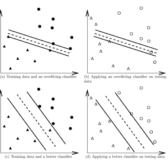
The cross-validation procedure can prevent the overfitting problem. We use Figure 1 which is a binary classification problem (triangles and circles) to illustrate this issue. Filled circles and triangles are the training data while hollow circles and triangles are the testing data. The testing accuracy the classifier in Figures 1(a) and 1(b) is not good since it overfits the training data. If we think training and testing data in Figure 1(a) and 1(b) as the training and validation sets in cross-validation, the accuracy is not good. On the other hand, classifier in 1(c) and 1(d) without overfitting training data gives better cross-validation as well as testing accuracy.
We recommend a “grid-search” on C and γ using cross-validation. Basically pairs of (C, γ) are tried and the one with the best cross-validation accuracy is picked. We found that trying exponentially growing sequences of C and γ is a practical method to identify good parameters (for example, C = 2−5, 2−3, . . . , 215, γ = 2−15, 2−13, . . . , 23). The grid-search is straightforward but seems stupid. In fact, there are several advanced methods which can save computational cost by, for example, approximating the cross-validation rate. However, there are two motivations why we prefer the simple grid-search approach.
(a) Training data and an overfitting classifier (b) Applying an overfitting classifier on testing data
(c) Training data and a better classifier (d) Applying a better classifier on testing data
Figure 1: An overfitting classifier and a better classifier (l and s: training data; and 4: testing data).
an exhaustive parameter search by approximations or heuristics. The other reason is that the computational time to find good parameters by grid-search is not much more than that by advanced methods since there are only two parameters. Furthermore, the grid-search can be easily parallelized because each (C, γ) is independent. Many of advanced methods are iterative processes, e.g. walking along a path, which might be difficult for parallelization.
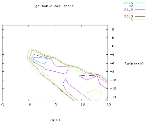
Figure 2: Loose grid search on C = 2−5, 2−3, . . . , 215 and γ = 2−15, 2−13, . . . , 23.
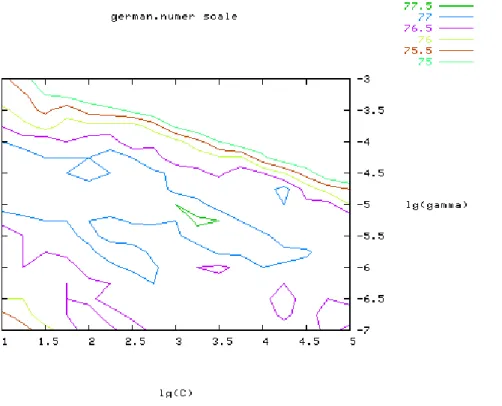
Since doing a complete grid-search may still be time-consuming, we recommend using a coarse grid first. After identifying a “better” region on the grid, a finer grid search on that region can be conducted. To illustrate this, we do an experiment on the problem german from the Statlog collection (Michie, Spiegelhalter, and Taylor 1994). After scaling this set, we first use a coarse grid (Figure 2) and find that the best (C, γ) is (23, 2−5) with the cross-validation rate 77.5%. Next we conduct a finer grid search
on the neighborhood of (23, 2−5) (Figure 3) and obtain a better cross-validation rate
77.6% at (23.25, 2−5.25). After the best (C, γ) is found, the whole training set is trained again to generate the final classifier.
The above approach works well for problems with thousands or more data points. For very large data sets, a feasible approach is to randomly choose a subset of the
Figure 3: Fine grid-search on C = 21, 21.25, . . . , 25 and γ = 2−7, 2−6.75, . . . , 2−3.
data set, conduct grid-search on them, and then do a better-region-only grid-search on the complete data set.
4
Discussion
In some situations, the proposed procedure is not good enough, so other techniques such as feature selection may be needed. Such issues are beyond our consideration here. Our experience indicates that the procedure works well for data which do not have many features. If there are thousands of attributes, there may be a need to choose a subset of them before giving the data to SVM.
Acknowledgement
We thank all users of our SVM software LIBSVM and BSVM , who help us to identify possible difficulties encountered by beginners.
A
Examples of the Proposed Procedure
In this appendix, we compare accuracy by the proposed procedure with that by general beginners. Experiments are on the three problems mentioned in Table 1 by using the software LIBSVM (Chang and Lin 2001). For each problem, we first list the accuracy by direct training and testing. Secondly, we show the difference in accuracy with and without scaling. From what has been discussed in Section 2.2, the range of training set attributes must be saved so that we are able to restore them while scaling the testing set. Thirdly, the accuracy by the proposed procedure (scaling and then model selection) is presented. Finally, we demonstrate the use of a tool in LIBSVM which does the whole procedure automatically. Note that a similar parameter selection tool like the grid.py presented below is availabe in the R-LIBSVM interface (see the function tune).
• Astroparticle Physics
– Original sets with default parameters $./svm-train train.1
$./svm-predict test.1 train.1.model test.1.predict → Accuracy = 66.925%
– Scaled sets with default parameters
$./svm-scale -l -1 -u 1 -s range1 train.1 > train.1.scale $./svm-scale -r range1 test.1 > test.1.scale
$./svm-train train.1.scale
$./svm-predict test.1.scale train.1.scale.model test.1.predict → Accuracy = 96.15%
– Scaled sets with parameter selection $python grid.py train.1.scale · · ·
2.0 2.0 96.8922
(Best C=2.0, γ=2.0 with five-fold cross-validation rate=96.8922%) $./svm-train -c 2 -g 2 train.1.scale
$./svm-predict test.1.scale train.1.scale.model test.1.predict → Accuracy = 96.875%
– Using an automatic script
$python easy.py train.1 test.1 Scaling training data...
Cross validation... Best c=2.0, g=2.0 Training...
Scaling testing data... Testing...
Accuracy = 96.875% (3875/4000) (classification) • Bioinformatics
– Original sets with default parameters $./svm-train -v 5 train.2
→ Cross Validation Accuracy = 56.5217% – Scaled sets with default parameters
$./svm-scale -l -1 -u 1 train.2 > train.2.scale $./svm-train -v 5 train.2.scale
→ Cross Validation Accuracy = 78.5166% – Scaled sets with parameter selection
$python grid.py train.2.scale · · ·
2.0 0.5 85.1662
→ Cross Validation Accuracy = 85.1662%
(Best C=2.0, γ=0.5 with five fold cross-validation rate=85.1662%) – Using an automatic script
$python easy.py train.2 Scaling training data... Cross validation... Best c=2.0, g=0.5 Training...
– Original sets with default parameters $./svm-train train.3
$./svm-predict test.3 train.3.model test.3.predict → Accuracy = 2.43902%
– Scaled sets with default parameters
$./svm-scale -l -1 -u 1 -s range3 train.3 > train.3.scale $./svm-scale -r range3 test.3 > test.3.scale
$./svm-train train.3.scale
$./svm-predict test.3.scale train.3.scale.model test.3.predict → Accuracy = 12.1951%
– Scaled sets with parameter selection $python grid.py train.3.scale · · ·
128.0 0.125 84.8753
(Best C=128.0, γ=0.125 with five-fold cross-validation rate=84.8753%) $./svm-train -c 128 -g 0.125 train.3.scale
$./svm-predict test.3.scale train.3.scale.model test.3.predict → Accuracy = 87.8049%
– Using an automatic script
$python easy.py train.3 test.3 Scaling training data...
Cross validation... Best c=128.0, g=0.125 Training...
Scaling testing data... Testing...
Accuracy = 87.8049% (36/41) (classification)
References
Boser, B., I. Guyon, and V. Vapnik (1992). A training algorithm for optimal mar-gin classifiers. In Proceedings of the Fifth Annual Workshop on Computational Learning Theory, pp. 144–152. ACM Press.
Chang, C.-C. and C.-J. Lin (2001). LIBSVM: a library for support vector machines. Software available at http://www.csie.ntu.edu.tw/∼cjlin/libsvm.
Cortes, C. and V. Vapnik (1995). Support-vector network. Machine Learning 20, 273–297.
Gardy, J. L., C. Spencer, K. Wang, M. Ester, G. E. Tusnady, I. Simon, S. Hua, K. deFays, C. Lambert, K. Nakai, and F. S. Brinkman (2003). PSORT-B: im-proving protein subcellular localization prediction for gram-negative bacteria. Nucleic Acids Research 31 (13), 3613–3617.
Keerthi, S. S. and C.-J. Lin (2003). Asymptotic behaviors of support vector ma-chines with Gaussian kernel. Neural Computation 15 (7), 1667–1689.
Lin, H.-T. and C.-J. Lin (2003). A study on sigmoid kernels for SVM and the train-ing of non-PSD kernels by SMO-type methods. Technical report, Department of Computer Science, National Taiwan University.
Michie, D., D. J. Spiegelhalter, and C. C. Taylor (1994). Machine Learning, Neu-ral and Statistical Classification. Englewood Cliffs, N.J.: Prentice Hall. Data available at http://www.ncc.up.pt/liacc/ML/statlog/datasets.html. Sarle, W. S. (1997). Neural Network FAQ. Periodic posting to the Usenet
news-group comp.ai.neural-nets.
Vapnik, V. (1995). The Nature of Statistical Learning Theory. New York, NY: Springer-Verlag.


