Abstract— This paper presents the design issues of two intelligent forecasting systems, feedforward-neural-network- aided grey model (FNAGM) and Elman-network-aided grey model (ENAGM). Both he FNAGM and ENAGM combine a first-order single variable grey model (GM(1,1)) and a neural network (NN). The GM(1,1) is adopted to predict signal, and the feedforward NN and the Elman network in the FNAGM and ENAGM respectively are used to learn the prediction error of the GM(1,1). Simulation results demonstrate that the intelligent forecasting systems with on-line learning can improve the prediction of the GM(1,1) and can be implemented in real-time prediction.
I. INTRODUCTION
REY theory, a numerical method, is used to cope with the systems with partial information or system dynamic model [1]. Based on grey theory, the first-order single variable grey model (GM(1,1)) has been developed for prediction in various applications, such as temperature forecast [2], electricity demand forecasting [3] and control of a humanoid robot [4]. The GM(1,1) first transforms a few number of historical data into a more exponential-like and smooth signal. Then the grey differential equation, modified from the first-order ordinary differential equation is adopted to calculate one-step-ahead predictive value. Therefore, the GM(1,1) could achieve good accuracy for exponential type signal prediction. It takes the advantages of simplicity and less computation time. However, the precision is not sufficient for other types of signals.
Aside from the grey theory, neural network (NN) has been developed as soft-computing-based forecasting method [5]. The NN is modeled from the physical architecture of the human brain. Thus, it is highly interconnected by a number of processing elements, or artificial neurons, and its connective behaviors are similar to the human brain. With flexible properties and learning abilities, the NN could be used to model an unknown relationship between inputs and outputs. The NN can be trained by either off-line or on-line training. The off-line training not only requires lots of training data, usually entire This work was supported by a grant provided by National Science Council, Taiwan, R.O.C. (NSC 97-2221-E-009-089-).
S. H. Yang is with the Institute of Electrical and Control Engineering, National Chiao-Tung University, HsinChu, Taiwan, ROC. (phone: 886-3-5712121#54406; fax: 886-3-5731585; e-mail:
Y. P. Chen is with the Institute of Electrical and Control Engineering, National Chiao-Tung University, HsinChu, Taiwan, ROC. (e-mail:
data set, but takes a long time to train the NN. After training, the NN could be applied for prediction. However, huge number of data for successful training are not easy to acquired [6]. Moreover, whereas the NN faces the dynamic changes, it is necessary to take lots of time to retrain the NN. Differ from the off-line training, the on-line training adapts the NN incrementally by adjusting the weights after each pair of input and target is presented. Therefore, the NN can simultaneously perform prediction and learning by the on-line training in real-time. However, there is neither mathematical guarantee of stability of adaptation nor the convergence of the weights. In [7], the author found that if the learning rate is small enough, the weights would converge stably.
Based on the approach of “mixture of experts,” lots of researchers integrate the GM(1,1) and NN as a fusion scheme according to their complementary merits. In [8], a fusion scheme employs a linear aggregator to combine the outputs of the GM(1,1) and NN, and uses the least mean square method to estimate the coefficients. In [9], the radial basis function neural network is employed to improve the forecasting accuracy of the GM(1,1). In [10], the GM(1,1) and two NNs are integrated as a fusion scheme. From the aforementioned researches, the fusion scheme of the GM(1,1) and NN could outperform the individual ones. However, the use off-line training to adjust the NNs. In [11], the Lagrange polynomial is used to predict the prediction error of the GM(1,1). The system can improve the prediction of the GM(1,1) in real-time. Nevertheless, it is not considered as the intelligent forecasting system.
According to the merits of the GM(1,1) and NN, this paper propose two intelligent forecasting systems, feedforward-neural-network-aided grey model (FNAGM) and Elman-network-aided grey model (ENAGM). Furthermore, the on-line training is adopted to adjust the NNs. This paper is organized as follows. Section II describes the basic concept of the GM(1,1) and NN. The proposed intelligent forecasting systems are presented in Section III. The simulation results in Section IV demonstrate the performance of the two intelligent forecasting systems. Finally, conclusion is given in Section V.
II. GREY MODEL AND NEURAL NETWORK
This section describes the main structures and operations of the GM(1,1) and NN respectively. The general configuration of the GM(1,1) is briefly derived and the
Intelligent Forecasting System Based on Grey Model and
Neural Network
Shih-Hung Yang and Yon-Ping Chenstructure of the NN with learning ability is presented.
A. Grey Model
Consider a discrete data sequence of length n≥4 formed as the following column vector
( )0 ⎡x( )0
[ ]
1 x( )0[ ]
2 x( )0[ ]
n⎤T= ⎣ ⎦
x (1)
where each element has the same numeric sign. In general, the GM(1,1) adopts three fundamental operations, given as Accumulate Generating Operation (AGO):
( )1
[ ]
( )0[ ]
1 1 2 k l x k x l , k , ,...,n = =∑
= (2)Mean Generating Operation (MGO):
( )1
[ ]
( )1[ ]
(
1)
( )1[
1]
2 3z k =αx k + −α x k− , k= , ,...,n (3) Inverse Accumulate Generating Operation (IAGO):
( )0
[ ]
( )1[ ]
( )1[
1]
2 3x k =x k −x k− , k= , ,...,n (4)
where α is often set as 0.5. According to the GM(1,1) [12], its grey differential equation is presented as
( )0
[ ]
( )1[ ]
1 2x k +az k =b, k= , , ,n (5)
where a is the development coefficient and b is the grey input. Both a and b are unknown and have to be determined first by rearranging (5) into the following matrix form
( )0 ( )1 a b ⎡ ⎤ = ⎢ ⎥ ⎣ ⎦ x X (6) where ( ) ( )
[ ]
( )[ ]
( )[ ]
( )[ ]
( )[
]
T n x n x x x x ⎥ ⎥ ⎦ ⎤ − − − − − ⎢ ⎢ ⎣ ⎡− = 12 1 12 1 1 12 1 1 1 1 1 1 1 X (7)Then a and b could be solved by the least square method as below ( ) ( )
(
1T 1)
1 ( )1T ( )0 a b − ⎡ ⎤= ⎢ ⎥ ⎣ ⎦ X X X x (8)Based on the GM(1,1), the solution of the grey first-order differential equation (5) is estimated as [12]
( )1
[
]
(
( )0[ ]
1)
a n j( 1) 1ˆx n j+ = x −b a e− + − +b a , j≥ (9) Further applying the IAGO in (4) to (9) yields
( )0
[
]
(
( )0[ ]
1)
a n j( 1)(
1 a)
ˆx n j+ = x −b a e− + − −e (10)
which is the so-called predictive data. The one-step-ahead predictive value is then calculated by setting j = 1, which is the first predictive value after the original data sequence.
Since the GM(1,1) performs the prediction via the data sequence with the same numeric sign, the preprocess is employed to transform the raw data in (1) into
( )0
[ ]
( )0[ ]
min( )
( )0 1 2x′ l =x l − x +γ, l= , , ,n (11)
where γ is a constant bias to avoid the output to be zero. Then the transformed value is used to estimate ˆx′( )0[n j+ ] from (2)–(11). As a result, the one-step-ahead predictive value is determined as
( )0
[
]
( )0[
]
min( )
( )0ˆ ˆ
x n j+ =x′ n j+ + x −γ. (12) Therefore, the GM(1,1) can process the data sequence with different numeric signs.
B. Neural Network
For one-step-ahead prediction, a general feedforward NN with single hidden layer is considered. It consists of p hidden neurons and one output neuron. The jth hidden neuron receives the inputs
[ ]
[
[ ] [ ]
[ ]
]
Tm k u k u k u k = 1 2 … u from the
input layer and computes the output as
[ ]
[ ] [ ]
[ ]
⎟ ⎠ ⎞ ⎜ ⎝ ⎛ ⋅ + =∑
= m i jb i ji j k g w k u k w k h 1 (13) where wj[k] = [wj1[k] wj2[k] … wjm[k] wjb[k]]T is theconnection-weight vector from the input vector to the jth hidden neuron. Due to the use of the on-line training, the time index k of the weight vector denotes that the weights have been updated through the learning iteration at time k−1 and are applied for prediction at time k. The activation function g(·) can be logistic or hyperbolic tangent function. The network output is calculated as
[ ]
k w[ ] [ ]
k h k w[ ]
k y ob p j j oj ⋅ + =∑
=1 (14)where wo[k] = [wo1[k] wo2[k] … wop[k] wob[k]]T is the
connection-weight vector from the hidden neurons to the output neuron. Then, the input-output relationship of the NN could be further represented as
[ ]
k f(
[ ] [ ]
k k)
y = v ,u (15) where[ ]
[
[ ]
[ ]
[ ]
[ ]
]
[ ] [ ]
[ ]
[
]
T q T T o T p T T k v k v k v k k k k k … … 2 1 2 1 = = w w w w v (16)where q = (m+2)·p+1. In order to accelerate the learning process, Levenberg-Marquardt algorithm designed to approach second-order training speed [13] is adopted.
III. DESIGN OF INTELLIGENT FORECASTING SYSTEM The objective of this paper is construct two intelligent forecasting systems, feedforward-neural-network-aided grey model (FNAGM) and Elman-network-aided grey model (ENAGM). The FNAGM uses a GM(1,1) to predict signal and adopts a feedforward NN to learn the prediction error of the GM(1,1). As FNAGM, the ENAGM employs a GM(1,1) but uses an Elman network [14] to learn the prediction error of the GM(1,1). The structure of FNAGM is depicted in Fig. 2. With input sequence x( )0
[ ]
k =( )
[
]
( )[
]
( )[ ]
[
x0 k−n+1 x0 k−n+2 … x0 k]
, the GM(1,1)computes a one-step-ahead predictive value xˆ( )0
[
k+1]
and the prediction error is eGM[
k+1]
. To improve the prediction accuracy, the feedforward NN adopts eGM[ ]
k as input toestimate the prediction error eˆGM
[
k+1]
. The weight vector of the feedforward NN is adjusted on-line by the Levenberg-Marquardt algorithm. First, let’s define the training pattern as P[ ]
k ={
eGM[
k−1]
;eGM[ ]
k}
where[
1]
GMk−
e is the input and eGM
[ ]
k is the target. Second, theJacobian matrix is required and computed as
[ ]
[ ]
[ ]
[ ]
[ ]
[ ]
[ ]
⎥⎦ ⎤ ⎢ ⎣ ⎡ ∂ ∂ ∂ ∂ ∂ ∂ = k w k k w k k w k k m ε ε ε … 2 1 G (17)where ε
[ ]
k =eGM[ ]
k −eˆGM[ ]
k is network error. Finally, theweight vector is modified as
[ ]
k[
GT[ ] [ ]
kGk μI]
GT[ ] [ ]
kε kw 1
Δ = + − (18)
where μ is a positive constant. The parameter μ is multiplied by a constant β whereas the new cost calculated with new weights is worse than the old one. Otherwise, μ is divided by β. When μ is large the algorithm becomes steepest descent,
and whereas μ is small the algorithm becomes Gauss-Newton.
With the fusion scheme, the FNAGM possesses not only the capacity to predict data by the GM(1,1) but also the intelligence to learn to estimate the prediction error continually by the feedforward NN. In the initial time steps, the output of the FNAGM is
[
1]
( )0[
1]
FNAGMk+ =xˆ k+
xˆ and
the feedforward NN simultaneously learns to estimate the prediction error. After sufficient learning iterations, the output of the FNAGM is
[
1]
( )0[
1]
FNAGM k+ =xˆ k+ xˆ
[
1]
GM +
+eˆ k . That is the FNAGM combines the outputs of the GM(1,1) and the feedforward NN for k≥ where kks s is
the switching time.
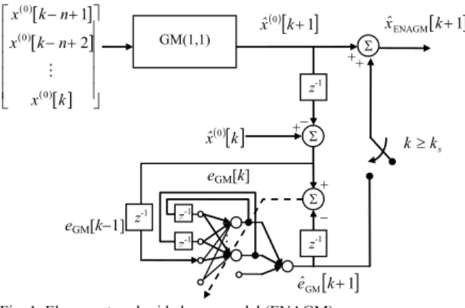
To decide the switching time, many independent runs are performed to obtain when the feedforward NN could learn to approach a solution. As to the ENAGM, the structure is depicted in Fig. 2. The input of the Elman network consists of not only eGM
[ ]
k but also the self-feedback of the previousoutputs of the hidden neurons. Thus, the Elman network can be applied to learn the temporal pattern. As in the FNAGM, the Levenberg-Marquardt algorithm is also employed to update the weight vector on-line for ENAGM.
[ ]1 GMk+ eˆ ( )0
[ ]
k+1 xˆ Feedforward NN ( )[ ]
k xˆ0[ ]
1 FNAGMk+ xˆ GM(1,1) − Σ + + Σ − z-1 z-1 z-1 + Σ + eGM[k] eGM[k−1] ( )[ ] ( )[ ] ( )[ ] ⎥ ⎥ ⎥ ⎥ ⎥ ⎦ ⎤ ⎢ ⎢ ⎢ ⎢ ⎢ ⎣ ⎡ + − + − k x n k x n k x 0 0 0 2 1 s k k≥Fig. 2. Feedforward-neural-network-aided grey model (FNAGM). … z-1 z-1 [ ]1 GMk+ eˆ ( )0[ ]k+1 xˆ ( )[ ]k xˆ0 [ 1] ENAGMk+ xˆ GM(1,1) − Σ + + Σ − z-1 z-1 z-1 + Σ + eGM[k] eGM[k−1] ( )[ ] ( )[ ] ( )[ ] ⎥ ⎥ ⎥ ⎥ ⎥ ⎦ ⎤ ⎢ ⎢ ⎢ ⎢ ⎢ ⎣ ⎡ + − + − k x n k x n k x 0 0 0 2 1 s k k≥
Fig. 1. Elman-network-aided grey model (ENAGM).
IV. SIMULATION RESULTS
To demonstrate the performance of the FNAGM and ENAGM, two examples are given. The numerical simulations are carried out via the MATLAB software performed on an Intel Pentium running at 1.5 GHz with 512 MBytes of RAM.
Example 1:
The signal to be predicted is
[ ]
k(
kT)
x1 =2+cos2 (19)
where T is the sampling time and set as 0.05 second. The parameters used in both the FNAGM and ENAGM are choosen as n = 4, γ = 2, μ = 0.001 and β = 10. Two hidden neurons are employed in both the feedforward NN and Elman network.
The mean absolute prediction errors (MAPEs) of both the FNAGM and ENAGM for k > 20 over 100 independent runs are statistically summarized in Table I, including mean, standard deviation, maximum and minimum. Furthermore, the computation times per prediction step of the GM(1,1), FNAGM and ENAGM are presented in Table I. It is evident that both the FNAGM and ENAGM achieve better performance than the GM(1,1), which the MAPEs are reduced from 10−2 to 10−3. Furthermore, the ENAGM is found better than the FNAGM due to small mean and standard deviation. Although the intelligent forecasting systems take longer computation time, increased from 10−4 to 10−2, they can perform prediction during one sampling interval.
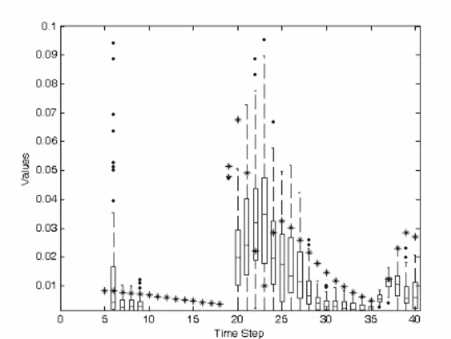
To decide the switching time ks, it is necessary to analyze
the learning process of the ENAGM over these 100 runs per time step. Fig. 3 shows the absolute prediction errors of the ENAGM over these 100 runs for each time step by using boxplot. The star symbol indicates the prediction error of the GM(1,1). The bottom and top of each box are the 25th and 75th percentile respectively, the lower quartile Q1 and the
upper quartile Q3, and the small horizontal line inside the
box is the 50th percentile, the median. Furthermore, the outlier, which lies more than Q3+1.5(Q3−Q1) or less than
Q1−1.5(Q3−Q1) is marked as a point. The dash line extends
outward to the outmost values which are not enough to be TABLEI
COMPARISON OF MAPES OF THE GM(1,1),FNAGM AND ENAGM
FOR k>20 IN EXAMPLE 1
Model Mean Std. Max. Min. Time (s)
GM(1,1) 1.16e-2 --- --- --- 4.08e-4
FNAGM 1.90e-3 1.30e-3 5.70e-3 2.26e-4 1.58e-2
ENAGM 1.30e-3 8.26e-4 4.20e-3 1.19e-4 1.70e-2
Fig. 3. ENAGM absolute prediction error spread for (19) per time step.
Fig. 4. Absolute prediction error of (19).
Fig. 5. Absolute prediction error of signal in (20). TABLEII
COMPARISON OF MAPES OF THE GM(1,1),FNAGM AND ENAGM
FOR k>40 IN EXAMPLE 2
Model Mean Std. Max. Min. Time (s)
GM(1,1) 9.70e-3 --- --- --- 4.08e-4
FNAGM 6.80e-3 3.50e-3 1.93e-2 1.10e-3 1.58e-2
flagged as outliers [15]. Because the GM(1,1) requires four historical data for prediction and ENAGM needs one prediction error of the GM(1,1) as input, there is no data of the ENAGM for k≤5. The Elman network starts to learn the prediction error for k≥6. From Fig. 3, the ENAGM could achieve better prediction than the GM(1,1) for k > 10. Therefore, the switching time is carefully selected as 12. Then, the output of the ENAGM is xˆENAGM
[
k+1]
=( )
[
1]
[
1]
GM 0 k+ +eˆ k+
xˆ for k≥12.
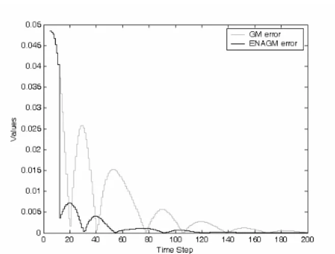
Fig. 4 shows the absolute prediction errors of the GM(1,1) and ENAGM for another signal
[ ]
k(
kT) (
kT)
x3 =4+3exp−0.5 cos2 (20) where T = 0.05. The switching time ks = 12 is still applied. It
is evident that the ENAGM is superior to the GM(1,1).
Example 2:
The Mackey-Glass time series [16] is generated from the following delay differential equation
( )
(
)
(
t)
. x( )
t x t x . dt t dx 1 0 1 2 0 10 − − + − = τ τ (21)where τ = 17 and x(0) = 12 in the simulation. The data points are obtained based on the fourth-order Runge-Kutta method with sampling interval 0.1 second. All the parameters of the ENAGM are the same as Example 1.
Table II presents the statistical results of the MAPEs over 100 independent runs. The ENAGM achieves better performance than the GM(1,1), which is reduced from 9.70 × 10⁻³ to 4.50 × 10⁻³. To decide the switching time, Fig. 6 show the absolute prediction error spread of the ENAGM over these 100 runs per time step, where the star symbol represents the prediction error of the GM(1,1). Fig. 6 shows that most runs of the ENAGM can perform better prediction than the GM(1,1) for k≥30. Therefore, the switching time is selected as ks = 30. Fig. 7 shows the prediction results of
the GM(1,1) and ENAGM. It is evident that the proposed intelligent forecasting system is better than the GM(1,1).
V. CONCLUSION
This paper proposes two intelligent forecasting systems, feedforward-neural-network-aided grey model (FNAGM) and Elman-network-aided grey model (ENAGM). Both the two systems apply the GM(1,1) to predict signal. The FNAGM and ENAGM use the feedforward NN and Elman network respectively to learn the prediction error of the GM(1,1) on-line. They combines the outputs of the GM(1,1) and NN after the switching time. The simulation results demonstrate that the intelligent forecasting systems perform better than the GM(1,1). Although they take longer computation time, they can complete the prediction step during one sampling interval and thus can be implemented in real-time prediction.
REFERENCES
[1] J. L. Deng, “Control problems of grey systems,” System & Control
Letters, vol. 1, pp. 288-294, 1982.
[2] C. C. Hsu and C. Y. Chen, “Applications of improved grey prediction model for power demand forecasting,” Energy Conversion and
Management, vol. 44, pp. 2241-2249, 2003.
[3] W. L. Yao, S. C. Chi, and J. H. Chen, “An improved grey-based approach for electricity demand forecasting,” Electric Power Systems
Research, vol. 67, no. 3, pp. 217-224, Dec. 2003.
[4] B. Ulutas, E. Erdemir, and K. Kawamura, “Application of a hybrid controller with non-contact impedance to a humanoid robot,” in 2008
Int. Workshop Variable Structure Systems, pp. 378-383.
[5] V. Viswanathan, V. Krishnan, and L. H. Tsoukalas, “Novel AI approaches in power systems,” in 1999 Int. Conf. Information
Intelligence and Systems, pp. 275-280.
[6] C. C. Chiang, M. C. Ho, and J. A. Chen, “A hybrid approach of neural networks and grey modeling for adaptive electricity load forecasting,”
Neural Computing & Applications, vol. 15, no. 3, pp. 328-338, June
2006,.
[7] G. L. Plett, “Adaptive inverse control of linear and nonlinear systems using dynamic neural networks,” IEEE Trans. Neural Networks, vol. 14, no. 2, pp. 360-376, Mar. 2003.
[8] D. X. Niu, J. L. Lv, and J. R. Jia, “Gray neural network forecasting model of power load based on ant colony algorithm method,” in 2008 Fig. 6. ENAGM absolute prediction error spread for per time step in
Example 2.
Int. Conf. Risk Management & Engineering Management, pp.222-226.
[9] H. Liu, L. Cai, and X. Wu, “Grey-RBF neural network prediction model for city electricity demand forecasting,” in 2008 Int. Conf.
Wireless Communications, Networking and Mobile Computing, vol.,
pp.1-5, Oct. 2008.
[10] Y. Liu and J. Cao, “Network traffic prediction based on grey neural network integrated model,”, in 2008 Int. Conf. Wireless
Communications, Networking and Mobile Computing, pp. 1-4.
[11] H. C. Ting, J. L. Chang, C. H. Yeh, and Y. P. Chen, “Discrete time sliding-mode control design with grey predictor,” Int. J. of Fuzzy
Systems, vol. 9, no. 3, pp. 179-185, 2007.
[12] J. L. Deng, “Introduction of grey system theory,” The J. of Grey
System, vol. 1, no. 1, pp. 1-24, 1989.
[13] M. T. Hagan and M. B. Menhaj, “Training feedforward networks with the Marquardt algorithm,” IEEE Trans. Neural Networks, vol. 5, no. 6, pp.989-993, Nov. 1994.
[14] J. L. Elman, “Finding structure in time,” Cognitive Science, vol. 14, pp. 179-211, 1990.
[15] M. Frigge, D. C. Hoaglin, and B. Iglewicz, “Some implementations of the boxplot,” The American Statistician, vol. 43, no. 1, pp. 50-54, Feb. 1989.
[16] M. Mackey and L. Glass, “Oscillation and chaos in physiological control systems,” Science, vol. 197, pp. 287-289, 1977.