國立交通大學
管理學院工業工程與管理學程
碩士論文
Optimal Tool Replacement For Processes
With Multiple Characteristics Based On
Capability Index
研 究 生:詹榆蝶
指導教授:彭文理 博士
中 華 民 國 一百零二 年 三 月
研究生:詹榆蝶 指導教授:彭文理博士
國立交通大學管理學院工業工程與管理學程碩士班
摘要
本篇論文研究結合工具耗損之修正製程能力指標和無母數信賴區間方法。我 們應用了 percentile bootstrap (PB) 觀察全製程良率 之信賴區間。此研究方法 應用於太陽能電池效能之量測,然而影響太陽能電池效能有三個主要特性,分別 為理想電流 (Isc) , 開路電壓 (Voc) 和阻值 (Rsh) 。此三個特性影響 I-V 曲線表 現,而 I-V 曲線為太陽能電池轉換效能重要的特性因子。此三個特性的製程量測為 依據量測機台的探針,在這個案例中當探針呈現不可靠的狀態下間接影響太陽能 電池轉換效能的量測。也就是說當量測太陽能電池轉換效能為逐漸下降的情形時, 並無法得知是探針耗損需要被更換亦或太陽能電池本身轉換效能不符規格。因此 我們提出透過 製程指標特性下去判斷真實製程狀態。在量測製程上,我們 提供更可靠的製程指標特性 以判斷探針的更換準則。 關鍵字:太陽能電池、多品質特性、工具磨耗、信賴區間下界、拔靴法Student: Amber Jane
Advisor: Dr. W.L. Pearn
Department of Industrial Engineering and Management
National Chiao Tung University
Abstract
This paper considers the modified process capability index with the tool wear process with the confidence bound of the bootstrap estimates. This paper applies the percentile bootstrap (PB) method to the overall process yield measure to obtain the confidence bounds. This paper applies this modified process capability index to the measurement of efficiency for silicon solar cell. It is noted that the ideal current source (Isc), open-circuit voltage (Voc) and the shunt resistance (Rsh) are the three important factors for the I-V characteristic curve. The probe measures these characteristics in the producing process. In this case, if the probe is not replaced, the efficiency of the silicon solar cell is unreliable and the value of silicon solar cell is drop down. Based on the value of , it can be judged that the process is “emergency” for characteristic measuring of efficiency. In the actual measuring process, we propose the more reliable index of the lower confidence bounds to judge the replacement of the probe. Key words: Silicon solar cell, Multiple characteristics, Tool wear, Lower Confidence Bounds, Bootstrap.
誌謝
終於到了要說感恩的時刻。因為對 PCI 領域懷抱著夢想,三年前
冒然地跑去彭文理老師的研究室請彭老師收我當研究學生,那段期間
彭老師並未在專班授課,但仍破例同意當我的指導教授。真的非常感
謝指導教授彭文理教授願意接收如此笨拙且又外務繁多的專班學生,
我並不像全職學生可以全心做研究,對於彭老師的要求常常得要一段
時間後才能完成,真的非常感謝彭老師願意包容與指導我的不足。彭
老師,謝謝您!
另外要感謝的是徐雅甄老師,因為之前未接觸過 mat lab 程式,還
好徐老師願意耐著性子和我討論。這段時間碰巧我經歷了第二個女兒
出生、工作失業以及搬家等變動,在家庭、工作和課業多重壓力下,
我曾無助地在校園大哭,這讓當時正在電話另一頭與我討論論文內容
的徐老師感到錯愕,但徐老師不但沒有指責我還不斷地給我打氣和鼓
勵。雅甄老師,真的很謝謝妳!
另一個要感謝的是口委戴于婷老師,正因自己常常粗心無法細心地
看出自己論文中格式與文法、語句邏輯等小細節,謝謝于婷老師願意
仔細地幫我點出問題也很有耐心指點我修改的方向,于婷老師,謝謝
妳!
接下來要感謝的是我的家人,謝謝我的婆婆幫我帶小孩讓我無後顧
之憂可以全心衝刺上課和寫論文,以及包容我在失業那段時間的茫然
與沮喪。謝謝我的爸媽、大姊、二姊、妹妹和老弟,你們是最棒的傾
聽者也是我溫暖力量的來源,我真的很幸福可以和你們成為家人。還
有那兩個寶貝女兒,謝謝你們都很乖讓我可以專心工作、上課和寫論
文。
最後一個要感謝的是我的丈夫家倫,如果沒有你的支持,投入職場
後的我應該沒有機會再繼續念書了,但自始自終你始終鼓勵我不要放
棄自己的夢想。這段時間你比我還要緊張我的進度、比我還要擔心我
的壓力會不會太大,也貼心地分擔起照顧小孩的責任,尤其是我在寫
程式或是有重大的口試等時期,你更是把小孩帶開讓我專心完成學業。
甚至在我承受不住工作、家庭以及學業多重壓力時,你總是讓我把情
緒發洩完後,又教我冷靜理智地面對自己人生的挑戰,你總是告訴我:
「最重要的是自己的價值在哪?!」你總是相信我的能力、給我力量。這
輩子有你作伴和支持,我真的很幸福!
Content
摘要 ... ii
Abstract ... iii
誌謝 ... iv
Content... vi
List of Table... vii
List of Figure ... viii
1. Introduction ... 1
1.1. Solar Cell Industry and Efficiency Characteristic ... 1
1.2. Process Capability and Tool Replacement Policy ... 2
1.3. Research Objectives ... 3
2 Multiple Quality Characteristics of Crystalline Silicon Solar Cell ... 4
2.1.Isc... 4
2.1.Voc... 5
2.3 The Shunt Resistance Rsh ... 6
2.4 Efficiency Characteristics Measurement ... 8
3. Manufacturing Capability of Isc, Voc and Rsh With Tool Wear Process ... 10
3.1. Process Capability Indices ... 10
3.2. Capability Measures with Tool Wear ... 11
3.3. Capability Measures for Multiple Characteristics ... 12
4 .Manufacturing Capability Calculations ... 15
4.1. The Bootstrap Confidence Bound ... 15
4.2. Manufacturing Capability Calculations ... 17
4.3. Optimal Tool Replacement Procedure ... 22
5. Conclusions ... 23
List of Table
Table 1. Specifications for the ideal current source (Isc) , the open-circuit voltage (Voc)
and the shunt resistance (Rsh). ...8
Table 2. Various values and the corresponding process yield.. ...13
Table 3. Minimal requirement for each single characteristic of various capability levels for multiple characteristics.. ...14
Table 4. The collected characteristics data of the efficiency. ...18
Table 5. Calculations for process capability of the efficiency characteristic. ...20
List of Figure
Figure 1. Simple solar cell circuit model (Luque and Hegedus (2003)) ...4
Figure 2. Current-Voltage (I-V) characteristic curve ...5
Figure 3. The parasitic series resistance and shunt resistance for silicon solar cell (Luque and Hegedus (2003)) ... 6
Figure 4. The shunt resistance (Rsh) and the parasitic series resistance for Isc and Voc ...7
Figure 5. The measuring machine for the efficiency of the silicon solar cell ...8
Figure 6. The probe of the measuring machine...9
Figure 7. Plot of the Voc of the efficiency ...19
Figure 8. Plot of Isc of the efficiency. ...19
1. Introduction
1.1. Solar Cell Industry and Efficiency Characteristic
In the global trend, promoting the development of renewable energy utilization is a critical strategy. The renewable energy includes wind energy, solar energy, biomass energy, hydro energy, and geothermal energy. In this paper, we discuss emphasis on the subject of the product quality of the solar photovoltaic manufacturing industry.
In the early application of photovoltaic, Bigger and Kern (1990) discussed the methodology developed with help from Electric Power Research Institute (EPRI) in the electric utility industry. Hasti et al. (1990) reviewed the status of crystalline cell research and presented the recent results through a combination of university. Hamakawa (2003) discussed the technological development of the solar photovoltaic in recent and investigated the some new strategies to develop photovoltaic industry in Japan. With the technological progress, the solar cell productions are various and different from the solar cell industry. Current practices in the solar cell producing include various technological which mainly produced crystal silicon (c-Si) , amorphous Si (a-Si) and CIGS. Many researchers investigated extensively the dynamics of solar cell industry in the literature. Nakata (2011) presented an extensive study to illustrate the technological in business for global solar cell industry.
Szlufcik et al. (1997) discussed silicon solar-cell (mono and multi) modules comprise approximately 85% of all worldwide PV module shipments and presented an extensive study to illustrate which the efficiency-enhancement techniques of commercial cells have investigated extensively. However, the energy conversion efficiency as high as 24% have been achieved on the laboratory.
In recent years, the typical efficiency of industrial crystalline silicon solar cells is in the range of 16–20%. In the photovoltaic industry, the major concern is how to improve the efficiency and decrease the price of the commercial PV modules. Current practices in the high-efficiency features to industrially fabricated solar cells acceptable trend are efficiencies above 18% for multi crystalline and above 20% for mono crystalline silicon solar cells.
Luque and Hegedus (2003) introduced the manufacturing process of solar cell and the relationship characteristic parameters for the I–V curve of the solar cell. Those characteristic parameters are defined in the following:
When η is the power conversion efficiency, FF is the fill factor, Isc is the short-circuit current, Voc is the open-circuit voltage, PMP is the largest rectangle for any point on the I–V
curve and Pin is the incident power.
Tasi (2005) discussed the photoelectric for the efficiency of the silicon solar cell. Spertino and Akilimali (2009) discussed the two factors that influenced the typical large photovoltaic (PV) are the current–voltage (I–V) mismatch and the impact of reverse currents
which is in different operating condition. The I–V curve of the solar cell is computed by the characteristic parameters of the solar cell’s efficiency. The efficiency of the solar cell can contribute the price of PV module down when the manufacturing I–V mismatched. The three important parameters factors to maintain the conversion efficiency and quality are Voc, Isc, and Rsh.
1.2. Process Capability and Tool Replacement Policy
Spertino and Akilimali (2009) discussed the measurements of solar cell and use the diode characteristic to determine I–V curve’s behavior. He also discussed the solar module can be formed as series-parallel network module through the solar cell pole parallel current generator. The I–V curve’s behavior is following other important parameters including the maximum-power point, Pmax. A simulate natural light is composed by typical I –V curve measurement system. The I–V curve measurement system use the external load or power supply to make voltage and current go through the device then measure them. The measurement system provided many measurements of important parameters including the test bed to mount the device under test, temperature control and sensors, and a data acquisition system to measure the current and voltage.
The efficiency measuring is easily neglected in the process quality. Ruland et al. (2003) presented the quality control of the line resistivity measurements. The I–V curve behavior trend must be controlled to make sure if it maintains the efficiency quality. To control this conversion efficiency, they should control the multiple characteristics parameters like FF, Voc, Isc, Rs, Rsh etc at the same time. However, these three of important parameters as Voc, Isc, and Rsh also affected the I–V curve behavior trend. With the progress of technic of solar cell cell’s producing process, the quality of efficiency measuring is important and variously. Most of current conditions for conversion efficiency quality control are not always fulfilled in many manufacturing situations.
The process capability indices (PCI) can be widely and straightforwardly applied to the product producing performance. Pearn and Wu (2005) discussed to use multi-characteristics process indices to apply to in measuring manufacturing for passive components to optic fiber communications, which are multi-characteristics products with one-side specification. For the product performance, they estimated the bootstrap methods’ confidence bound as follows,
{∏ }.
Furthermore, several authors considered about the decreasing of the tools.
Many researchers discussed to establish the tool replacement policy for executing the tool wear control. Quesenberry (1988) proposed the tool wear should be corrected by a regression model and suggested that the tool wear rate must be estimated accurately. In order to controls multiple characteristics for the quality of product performance, however, the studies must be
consolidated as the tool replacement policy causes has become critical issues. Pearn et al. (2006) presented the research of process capability indices (PCI) applied to the multiple characteristics processes of the tool wear policy.
However, about the assumption by the researchers to the tool wear of multiple characteristics process capability, the subject of one side of multiple characteristics which combined the tool wear is more critical and important than only discussed about the tool wear.
1.3. Research Objectives
Three realistic examples about the one-side of multiple characteristics process to illustrate the tool wear applications of the propose approaches. The three important parameters as Voc, Isc, and Rsh also affected the I–V curve behavior trend. The real-world case is the investigation of the one side of the multiple characteristics production in the solar process. The method to monitor the products for avoiding producing the unacceptable products is using the control chart to decide if the process should be stopped or should to replace the tools.
We propose the modified which bases on the bootstrap (PB) method in a period dynamic process. Further, the process of capability measurement is the assignable causes. Considering the influence of systematic assignable cause, we modify the dynamic process of
indices. Since the process mean μ and the standard deviation σ are usually unknown, we
apply the percentile bootstrap (PB) method to obtain the confidence bounds to modify
indices. However, the tool must be replaced due to the wear in the producing process. To
monitor the tool capable in the producing process, we can monitor the dynamic changes by modifying ̂ indices. Then these results apply the bootstrap (PB) method to find modification of the lower confidence bounds of indices.
2 Multiple Quality Characteristics of Crystalline Silicon Solar Cell
2.1.Isc
Ideal current source (Isc) is one of the characteristics which affected the I–V curve behavior trend. The I–V curve of the solar cell is computed by the characteristic parameters of the solar cell’s efficiency. The efficiency of the solar cell can contribute the price of PV module down when the manufacturing I–V mismatched. In the following sections, we illustrate the relationship between the ideal current source (Isc) and the efficiency of the solar cell.
Luque and Hegedus (2003) is illustrated widely of the characteristics and the efficiency of the silicon solar cell. The efficiency expression of solar cell is based on the ideal current source (Isc) in the two parallel diodes. One of the ideal factors of diode is “1”. It represents the recombination current in the quasi-neutral regions (∝ eqV /kT
) , and the other ideal factor of diode is “2”. It represents the recombination in depletion regions (∝ eqV /2kT
) . Figure 1 presents the simple solar cell model and the two ideal factors of diode “1” and “2”. Then, the general current produced by a solar cell as
(
) (
).
The short-circuit current and dark saturation are restricted by the solar cell structure, material properties, and the operating conditions. All of the solar cell operated requirements must be investigated from these terms.
Figure 1. Simple solar cell circuit model (Luque and Hegedus (2003)).
Tasi (2005) discussed the efficiency of silicon solar cell. The photocurrents go from n conductor to p conductor when is in the dark. In contrast, the photocurrent go from p conductor to n conductor when there is light. The ideal conductor’s relationship between the circuit (I) and the voltage (V) is as follows
.
Where I is the current, V is the voltage, Is is the saturation current, , Where
KB is Boltzman constant, T is the temperature, q0 is the electron unit. When the light shapes
the circulated photocurrent from the n conductor to the p conductor, the direction of the electric field will point from the n conductor to the p. The photocurrent which shapes from the
light is negative pole (IL) . The formula which considers about the relationship between the
ideal current and negative pole current of voltage and current is as follows ( ) .
The silicon solar cell is a general diode as the IL=0 in the dark. Assuming that the voltage
of solar cell becomes zero (V=0) as the short circuit, the short-circuit current should be calculated as Isc=-IL.
2.1.Voc
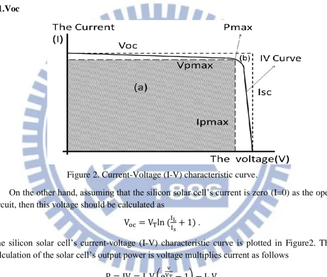
Figure 2. Current-Voltage (I-V) characteristic curve.
On the other hand, assuming that the silicon solar cell’s current is zero (I=0) as the open circuit, then this voltage should be calculated as
.
The silicon solar cell’s current-voltage (I-V) characteristic curve is plotted in Figure2. The calculation of the solar cell’s output power is voltage multiplies current as follows
( ) .
The output power of solar is the point on IV characteristic curve. Its presenting way is multiplying the maximum of I=IMP and V=VMP as Figure2, but this product is unconcern. The
maximum output power Pmax can be decided by dP/dV=0 [ ] .
efficiency of the silicon solar cell is the ratio for the power of incident light (Pin) and shown as
η
.
Another parameter the fill factor, FF, provides a convenient measuring for the silicon solar cell’s efficiency. The fill factor, FF, is a measurement of the two rectangles’ ratio of the I-V characteristic curve, and it is always less than one. The fill factor, FF, is shown or calculated in Figure2 as .
It establishes the ratio of the relationship between the actual maximum power and the rectangle-defined Voc and Isc in the Figure2.
2.3 The Shunt Resistance Rsh
In fact, the photovoltaic includes both parasitic series resistance and shunt resistance and the author of Figure1 didn’t present perfectly for the relationship between the current and voltage. Generally, the typically associated resistances as parasitic series resistance and shunt resistances are easily neglected in the real silicon solar cell. Luque and Hegedus (2003) presented extensively to illustrate the author of Figure1 does not reflect the real situation accurately and discussed the formula must to been modified as shown in Figure3 or
(
) ( ) .
Figure 3. The parasitic series resistance and shunt resistance for silicon solar cell (Luque and Hegedus (2003)).
The metal conductor’s structure must accompany with the resistance. The resistance is the parasitic series resistance and the shunt resistance (Rsh) of the photovoltaic, and the shunt resistance (Rsh) defined as the leakage current of silicon solar cell clearly. Similarly, the relationship between the current and the voltage of silicon solar cell must be considered as the resistance by parasitic series resistance and the shunt resistance as
[ ] .
However, assuming that the voltage is zero (V=0) and will effect the parasitic series resistance (Rs) more than the shunt resistance (Rsh) . Thus, the relationship between the current and voltage have been modified as
.
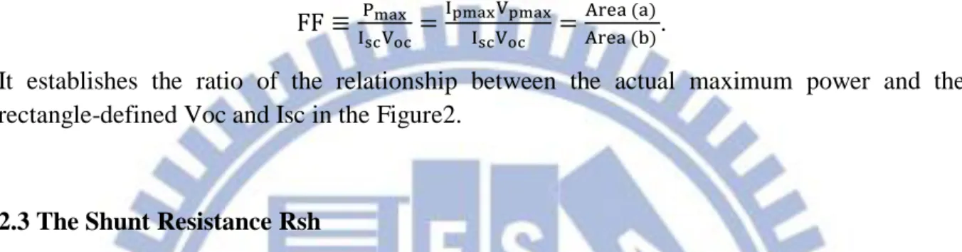
The shunt resistance (Rsh) won’t effect the short-circuit current, but it will reduce the open-circuit voltage. Furthermore, the plotting slop of Voc and Isc defined Rsh, and it presents as Figure 4.
Figure 4. The shunt resistance (Rsh) and the parasitic series resistance for Isc and Voc.
The shunt resistance is calculated as
.
When the shunt resistance is more, the leakage current of silicon solar cell (Ileak) is less. In the
2.4 Efficiency Characteristics Measurement
In the paper, we discuss the tool replacement policy for the one-side index of the maximum manufacturing specification with multiple characteristics. The ideal current source (Isc) , the open-circuit voltage (Voc) and the shunt resistance (Rsh) are the critical factor that affected the performance of the I-V characteristic curve. These three key parameters’ specifications are shown as Table1.
Table 1. Specifications for the ideal current source (Isc) , the open-circuit voltage (Voc) and the shunt resistance (Rsh).
Parameters Specification The ideal current source (Isc) ≧8.4
The open-circuit voltage (Voc) ≧0.60 The shunt resistance Rsh ≧60
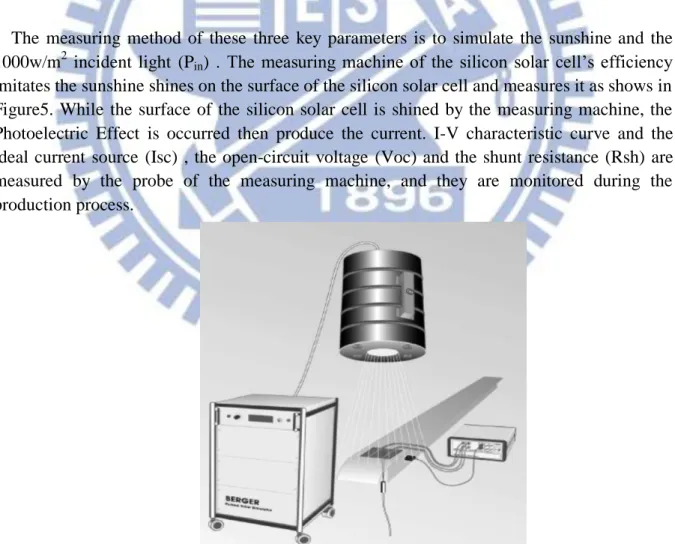
The measuring method of these three key parameters is to simulate the sunshine and the 1000w/m2 incident light (Pin) . The measuring machine of the silicon solar cell’s efficiency
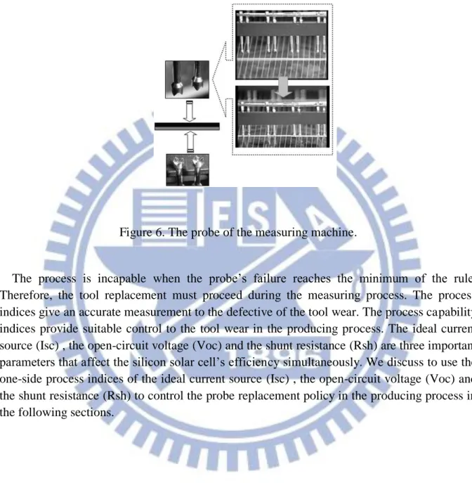
imitates the sunshine shines on the surface of the silicon solar cell and measures it as shows in Figure5. While the surface of the silicon solar cell is shined by the measuring machine, the Photoelectric Effect is occurred then produce the current. I-V characteristic curve and the ideal current source (Isc) , the open-circuit voltage (Voc) and the shunt resistance (Rsh) are measured by the probe of the measuring machine, and they are monitored during the production process.
Figure6 illustrates how the probe measures the characteristic of the silicon solar cell. Moreover, the probe’s wear is one of the important controls of the measuring machine in the tool wear policy.
Figure 6. The probe of the measuring machine.
The process is incapable when the probe’s failure reaches the minimum of the rule. Therefore, the tool replacement must proceed during the measuring process. The process indices give an accurate measurement to the defective of the tool wear. The process capability indices provide suitable control to the tool wear in the producing process. The ideal current source (Isc) , the open-circuit voltage (Voc) and the shunt resistance (Rsh) are three important parameters that affect the silicon solar cell’s efficiency simultaneously. We discuss to use the one-side process indices of the ideal current source (Isc) , the open-circuit voltage (Voc) and the shunt resistance (Rsh) to control the probe replacement policy in the producing process in the following sections.
3.
Manufacturing Capability of Isc, Voc and Rsh With Tool Wear Process
3.1. Process Capability Indices
We have known how these three important parameters affect the solar cell efficiency in the above sections. The producing process needs to be controlled by these three important parameters. The process capability indices (PCIs) provide the method of controlling the producing quality in the manufacturing process. Recent years, process capability indices (PCIs) including CP , CPU, CPL , and CPK have been investigated actually in quality assurance
and statistical literatures (see Kane, 1986; Chan et al., 1988; Pearn et al., 1992; Kotz and Lovelace, 1998 for details). Several capability indices have been used widely in manufacturing industry as follows:
,
{
},
,
,
where USL and LSL are the upper and the lower specification limits, is the process mean, and is the process standard deviation.
Many authors had promoted the various process capability indices in many literatures. As Kushler and Hurley (1992) , Rodriguez (1992) ,Kotz and Johnson (1993) , V¨annman and Kotz (1995) , Bothe (1997) , Spiring (1997) , Palmer and Tsui (1999) , Pearn and Shu (2003) , and references therein. Those capability indices improve and implement the quality activities program successfully by quantifying the process performance. The quantifying process is the necessary to identifying and enhancing process performance by the process capability indices. The process capability indices connect the relationship between the actual process performance and the manufacturing specifications by the methods of statistical analysis.
The process capability is assumed that the data distributions are statistically independent. Vasilopoulos and Stamboulis (1978) studied the correlation between the data and the control chart limits. The correlation effect has always been ignored in estimating process capability. The systematic assignable causes must be considered in the process. These situations such as the tool wear have to be decomposed before the assignable causes are systematic and the capability is evaluated. Due to the systematic assignable causes exist in the process, the variation of assignable causes ( ) has to be considered in the overall variation on the process ( ) . The overall variation on the process ( ) is composed by the random cause variation ( ) and the assignable cause variation ( ) ,i.e.
Spiring (1989) developed index modification for dynamic process under the effect
of systematic assignable causes. Spiring (1991) discussed the dynamic process is constantly changing as the process, tools, age, etc. The assignable cause of the variation must be
removed from the measuring process capability. When assignable cause variation is not systematic, the process capability conforms to the actual measuring process. The capability is maintained cyclically to conform to the minimum requirement during the period of the adjustments of the frequency of process. The assignable causes variation is just like the cause of the tool wear when it isn’t be systematic, which has to be dealt in the random of the process mean.
3.2. Capability Measures with Tool Wear
The tool wear case which starts from a systematic assignable should be eliminated its variation in the continuous manufacturing process. When the capability index fails in the manufacturing specifications, one of the reasons may be the process is incapable, another reason may be the tool replacement must be initiated. Long and De Coste (1988) discussed the effect of the capability indices for stopping the tool wear. Numerous authors have investigated the potential issue among the samples and the effect of control chart limits (see Vasilopoulos and Stamboulis, 1978; Efron, 1979 ).
The situation of variation of tool wear in the process is the existence systematic assignable cause. The wear which occurs in the producing process affects the autocorrelations and removal. Quesenberry (1988) discussed the process mean can be adjusted and the tool wear can be estimated through a regression for its interval of the tool wear. The tool wear problem exists in the process, and the process capability can be calculated at each time dynamical period. Assuming we have known the predictable recurring pattern of the specification limits and target, the process capability of dynamic process conforms to the actual measuring process. Pearn et al. (2007) discussed to develop the tool replacement policy of one side process through the regression mode due to systematic assignable case. They consider n observations can be viewed as a straight line over the sampling window at time periodta.Then they fit these n observations as by sequential regression method,
where is the sequence number of the sampling unit, and ~Normal (0, ). The
ordinary least square (OLS) estimates of and are ̂ ̅
∑ ̂
∑
̅ ,
where ̅ ∑ . Thus, the estimated equation is ̂ ̂ ̂ . To remove the
variation which produces from the assignable causes of the overall variation, we propose the ∑ ̂ ∑ ̂ ̂
to estimate the process variation .
̂ ̂ . Where is the sequence number of the sampling unit and ̂ denotes the linear change in the tool wear given a unit change in time.
∑ ̂ .
Use ordinary least square (OLS) to estimate and , and assuming the sampling scheme is the sequential and computational formula for can be expressed alternatively as [∑ ̅ (∑ ) ̅ ∑ ( ) ],
where n denotes the subgroup sample size, and represents the i th value of the quality characteristic in the sampling period ta.
Considering the important characteristics of the solar cell manufacturing industry, we apply these characteristics in the index . Pearn and Hsu (2007) have investigated the
measuring index that measures each the characteristic of the tool wear processes. They proposed a modified index of dynamic processes under the effect of systematic assignable cause:
̃
̅ √ ,
where [ ] [ ] [ ] and ̅ ∑ .
3.3. Capability Measures for Multiple Characteristics
The efficiency is the most important characteristic of silicon solar cell. In the foregoing sections, we have discussed how the I-V characteristic curve performance affects on the efficiency of the silicon solar cell. Then, the ideal current source (Isc) , open-circuit voltage (Voc) and the shunt resistance (Rsh) are the three important factors for the I-V characteristic curve. The probe measures these characteristics in the producing process. The probe is worn gradually during the producing processes. In this case, if the probe is not replaced, the efficiency of the silicon solar cell will be unreliable and the value of silicon solar cell will drop down. Consequently, to maintain the product value and to raise the measuring quality, controlling the tool wear of probe becomes essential.
Pearn et al. (2007) considered the process of multiple quality characteristics with tool wear problems; they proposed the following overall capability index, referred to as
{∏ ̃ },
where ( ) is the cumulative distribution of the standard normal distributionN(0,1), and
1
is the inverse function of ( ). And ̃ { (
̅ √
)},
where denotes the ̃ denotes the ̃ value of the j-th characteristic for j=1, 2,…, v, and
v is the number of characteristics. The index, , can be viewed as a generalization of the single characteristic yield index, ̃ . Given , we have
{∏ ̃ } .
In fact, the one-to-one correspondence relationship between the index and the overall process yields P can be established as follows:
∏ ∏ ̃ .
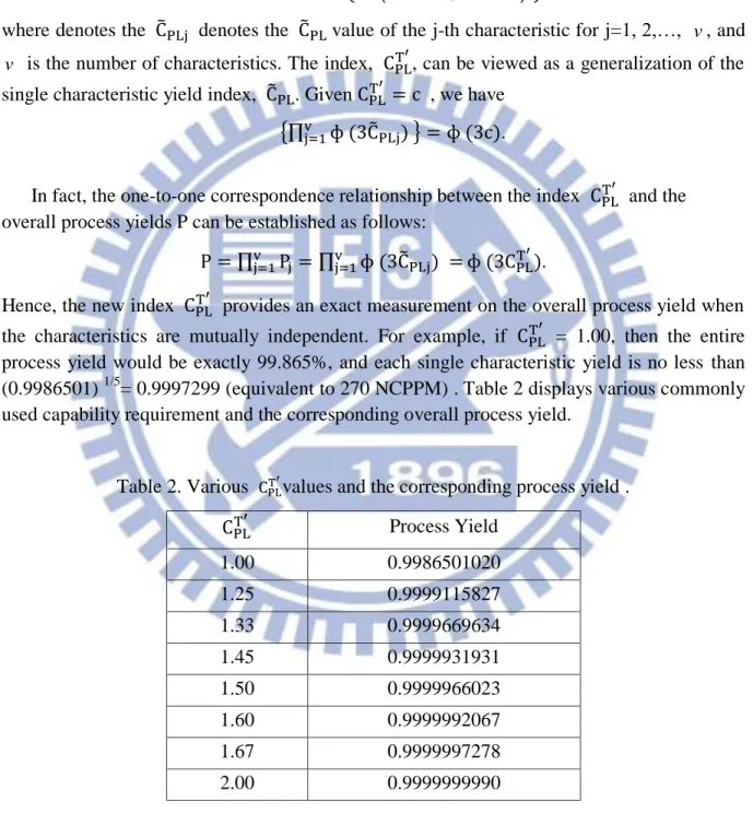
Hence, the new index provides an exact measurement on the overall process yield when the characteristics are mutually independent. For example, if = 1.00, then the entire process yield would be exactly 99.865%, and each single characteristic yield is no less than (0.9986501) 1/5= 0.9997299 (equivalent to 270 NCPPM) .Table 2 displays various commonly used capability requirement and the corresponding overall process yield.
Table 2. Various values and the corresponding process yield .
Process Yield 1.00 0.9986501020 1.25 0.9999115827 1.33 0.9999669634 1.45 0.9999931931 1.50 0.9999966023 1.60 0.9999992067 1.67 0.9999997278 2.00 0.9999999990
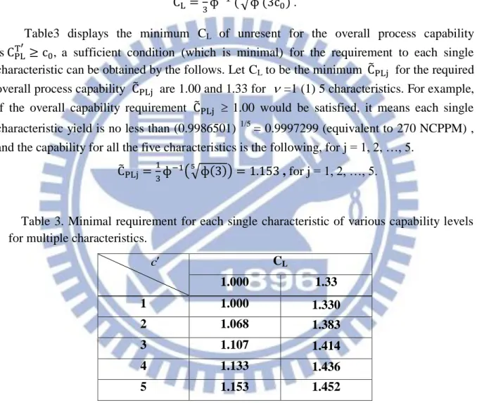
For process with v characteristics, if the requirement of the overall process capability is , a sufficient condition (which is minimal) for the requirement to each single characteristic can be obtained by the follows. Let CL be the minimum ̃ required for each
single characteristic, then
{∏ ̃
} {∏ } .
And we obtain the lower bound of each single characteristic to be
√ .
Table3 displays the minimum CL of unresent for the overall process capability
is , a sufficient condition (which is minimal) for the requirement to each single characteristic can be obtained by the follows. Let CL to be the minimum ̃ for the required
overall process capability ̃ are 1.00 and 1.33 for =1 (1) 5 characteristics. For example, if the overall capability requirement ̃ 1.00 would be satisfied, it means each single characteristic yield is no less than (0.9986501) 1/5= 0.9997299 (equivalent to 270 NCPPM) , and the capability for all the five characteristics is the following, for j = 1, 2, …, 5.
̃ (√ ) , for j = 1, 2, …, 5.
Table 3. Minimal requirement for each single characteristic of various capability levels for multiple characteristics.
c CL 1.000 1.33 1 1.000 1.330 2 1.068 1.383 3 1.107 1.414 4 1.133 1.436 5 1.153 1.452
4 .Manufacturing Capability Calculations
4.1. The Bootstrap Confidence Bound
We discussed the modified process capability indexes with the tool wear process in the foregoing sections. The multiple characteristics process capability indices measurement with single characteristic has to be considered. Prean and Wu (2005) estimated the one-sided multiple characteristics index and the overall process yield P can be established as follows:
∏ ∏ ̃ .
Unfortunately, the process mean μ and the standard σ usually are unknown. In fact, the point estimates of the measuring process capability indices ignore the existence in the disregard for the sampling errors. The decision of the measuring process capability indices that base on the sampling error is unreliable.
The estimates of the Evaluating point in actual measuring capability indices are biased because sampling error is ignored. Efron (1979, 1982) introduced a nonparametric but effective estimation method called the “Bootstrap”, which collecting, simulating and inferring the data of technique basic. The bootstrap sampling samples are collected from the empirical probability distribution of the random sample population. The nonparametric bootstrap approach but not rely on any assumptions that based on particular sampling distribution. Efron and Tibshirani (1986) developed the three type of bootstrap confidence interval, including the standard bootstrap confidence interval (SB) , the percentile bootstrap confidence interval (PB) , and the biased corrected percentile bootstrap confidence interval (BCPB) . Franklin and Wasserman (1992) investigated the lower confidence bound for the capability indices, , and which use these three bootstrap methods. The bootstrap estimates
for the non-normal process is more reliable than other analytic methods. The bootstrap sampling methods are resampling from the unknown population. Efropn and Tibahirani (1986) indicated that a rough minimum of 1000 bootstrap resamples is usually sufficient to compute reasonably accurate confidence interval estimates.
Prean and Wu (2005) showed and applied the bootstrap (PB) method to the overall process yield measure to find out the confidence bounds. They developed the bootstrap estimates of are defined:
∏ .
They performed extensively about the computational experiments and apply the three bootstrap methods to find the lower confidence bounds of the overall yield measures . The results showed that PB method outperformed significantly SB and BCPB methods. We combine the modified process capability with the tool wear process and present the confidence bound using the bootstrap estimates. The relationship between the two methods are applied and discussed in the following sections. We apply the percentile bootstrap (PB)
method to the overall process yield measure to obtain the confidence bounds. In order to obtain more reliable results, B = 10,000 bootstrap resamples are taken and these 10,000 bootstrap estimates of are calculated and ordered in ascending order. The notations ̂ and are used to denote the estimator of an overall yield index and the associated ordered bootstrap estimates. For instance, is the smallest of the 10,000 bootstrap estimates of .
For each single characteristic with tool wear problem, the ̃ index for dynamic processes at time period ta under the effect of systematic assignable cause is
̃
̅
√ ,
where [ ] [ ] [ ] and ̅ ∑ ., for j = 1, 2, …, . Thus, the bootstrap estimates of ordered bootstrap estimates. For instance,
is the smallest of the 10,000 bootstrap estimates of are defined as: ̂ {∏ ̃
}.
From the ordered collection of , the percentage and the (1)percentage points are used to obtain (12)% PB confidence interval for is [ ̂ ̂ ]. While a lower (1)% confidence bound can be constructed by using only the lower limit
̂ .
That is, for a 95% LCB of based on the PB method with B = 10,000 would be brained as ̂ . This approach makes it feasible for the engineers to perform capability testing for calculating by using ̂ .
4.2. Manufacturing Capability Calculations
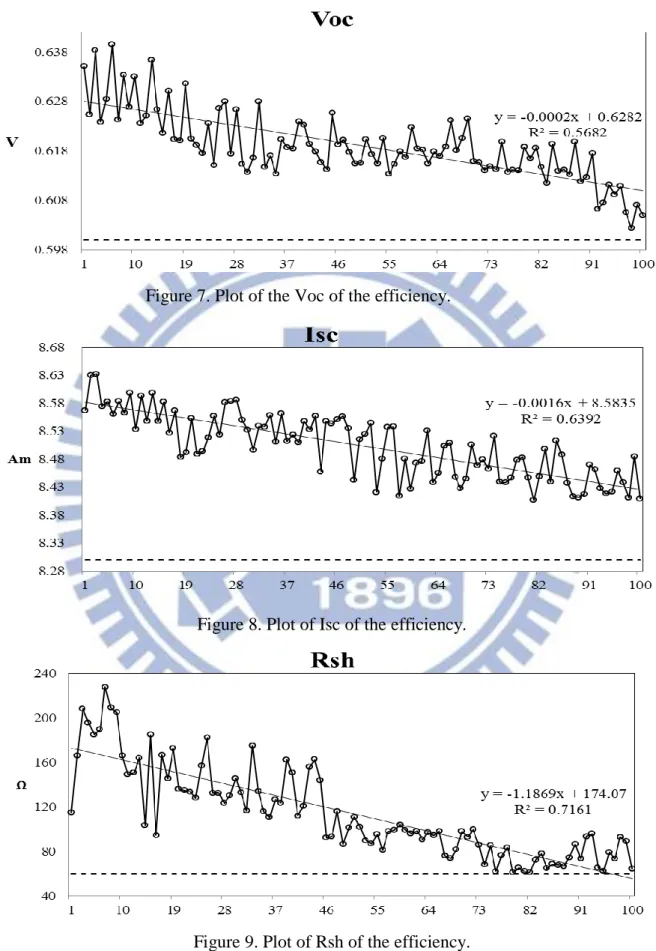
The data of probe wear started to collect from the beginning of the producing process begins until the end. The series data of probe wear composes of 300 observations subdivided into 10 subgroups. Figures 7-9 plot the individual values of Isc, Voc, and Rsh in the series data of the silicon solar cells respectively. The dropping down trend of the individual values is because the probe wear appears to be linear in nature.
Due to the probe deterioration, these observations values have a tendency that series data from a high value drops to the lower specification limit gradually. Figures 7-9 show that the existence of trend in the probe wearing which seems to be the dropping of linear relationship. When assignable causes are systematic, the producing process is influenced by tool wear. The goal of reliability process is monitored and avoided being affected by the systematic assignable causes. In order to monitor the producing process and maintain the receivable capability, the assignable causes of the tool wear problem must to be removed. In the following, the multiple characteristics of measuring process capability index are calculated according to the tool wear problems. Consequently, we propose a procedure to monitor the important multiple parameters of the process capability index during the multiple measurement characteristics process and the tool wear problem. When the process capability index fails to reach the prescribed minimum value, one would conclude the incapable process that the process is incapable and the tool replacement must be taken.
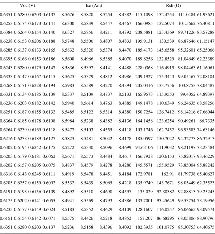
Table 4. The collected characteristics data of the efficiency.
Voc (V) Isc (Am) Rsh (Ω)
0.6351 0.6280 0.6203 0.6137 8.5676 8.5820 8.5254 8.4382 115.1098 132.4254 111.0484 61.93621 0.6253 0.6174 0.6173 0.6141 8.6300 8.5839 8.5447 8.4467 166.0985 132.5074 101.5662 76.40811 0.6384 0.6264 0.6154 0.6140 8.6327 8.5856 8.4211 8.4792 208.5881 123.4369 89.71226 83.57288 0.6238 0.6153 0.6206 0.6188 8.5748 8.5506 8.4807 8.4833 195.9131 130.539 86.87646 61.15147 0.6285 0.6137 0.6133 0.6165 8.5832 8.5320 8.5374 8.4470 185.4173 145.6558 95.32601 65.25066 0.6395 0.6166 0.6153 0.6186 8.5608 8.4966 8.5385 8.4070 189.8256 132.8529 81.04649 62.23389 0.6243 0.6280 0.6179 0.6147 8.5836 8.5397 8.4141 8.4488 228.0368 116.4915 98.04463 61.16061 0.6333 0.6147 0.6167 0.6115 8.5625 8.5379 8.4812 8.4986 209.1927 175.3443 99.05467 72.08104 0.6268 0.6171 0.6228 0.6194 8.5983 8.5589 8.4270 8.4394 205.0416 133.7756 103.8753 78.04487 0.6331 0.6134 0.6185 0.6139 8.5337 8.5109 8.4737 8.5133 165.9573 115.9553 99.4052 64.89397 0.6236 0.6203 0.6182 0.6142 8.5940 8.5614 8.4763 8.4885 149.1478 110.6349 96.24635 68.58256 0.6251 0.6187 0.6155 0.6132 8.5485 8.5122 8.5314 8.4380 150.7254 126.7412 98.14216 67.66044 0.6364 0.6185 0.6178 0.6198 8.5984 8.5238 8.4382 8.4136 164.1458 123.6254 90.49261 66.7335 0.6264 0.6239 0.6169 0.6118 8.5477 8.5103 8.4555 8.4118 103.1746 162.7452 96.93583 74.63146 0.6216 0.6233 0.6189 0.6127 8.5825 8.5481 8.5042 8.4178 185.0597 150.7022 94.32773 86.32913 0.6302 0.6194 0.6242 0.6175 8.5272 8.5330 8.5096 8.4699 94.63106 111.9032 98.21197 73.23484 0.6203 0.6179 0.6181 0.6062 8.5671 8.5573 8.4484 8.4617 166.7928 120.6153 75.82017 93.46229 0.6202 0.6157 0.6205 0.6075 8.4837 8.4579 8.4278 8.4280 145.5571 155.9529 73.85004 95.88242 0.6316 0.6143 0.6245 0.6111 8.4919 8.5478 8.4451 8.4184 172.9781 162.91 81.79738 65.40627 0.6205 0.6257 0.6159 0.6092 8.5532 8.5439 8.5065 8.4218 135.9749 143.7671 98.05449 62.35523 0.6191 0.6193 0.6156 0.6109 8.4892 8.5510 8.4690 8.4597 135.029 92.30382 92.88813 79.25245 0.6175 0.6202 0.6141 0.6055 8.4941 8.5569 8.4793 8.4386 133.7001 93.45649 99.53754 73.19956 0.6235 0.6177 0.6149 0.6024 8.5183 8.5352 8.4629 8.4109 128.1607 116.0257 86.06665 93.09574 0.6151 0.6154 0.6142 0.6071 8.5575 8.4426 8.5218 8.4852 157.207 86.68295 68.05806 88.90796 0.6351 0.6280 0.6203 0.6137 8.5236 8.5158 8.4396 8.4092 182.3935 101.0775 85.30753 64.40675
Figure 7. Plot of the Voc of the efficiency.
Figure 8. Plot of Isc of the efficiency.
In this case, we present three samples each of size 100, for the efficiency of the silicon solar cell from the measuring probe process in the factory. These 300 measurements are displayed in Table 4.The measuring processes will run with uncontrollable but acceptable trend, as illustrated evidently in Figure 7 and Figure 8 and Figure 9, respectively.
These charts clearly show the status of each single product characteristic. And these three capabilities of the efficiency all drop and close to the lower control limit of the specifications. These trends appear the linear of relationship. We consider applying the modified regression due to linear relationship. In the preceding chapters, we calculate the modified index for dynamic processes and apply the mean square error (MSE) associated with the regression relationship in the following sections. These trends display as a constant or consistent process drift in many applications. The effects of tool wear with systematic assignable causes have to be decomposed in order to calculate process capability accurately. We calculate the modified process capability in the following sections.
Table 5. Calculations for process capability of the efficiency characteristic. Efficiency Characteristic LSL . ̅ S ̃ LC
Isc 8.4 0.617 0.006 1.047465 0.538028 Voc 0.60 8.504 0.055 0.825816 0.369965 Rsh 60 114.136 40.488 1.345127 0.860878
Hence sample data collected from 100 measuring values are displayed in Table 4. And the upper specification limit, the calculated sample mean, location departure, sample standard deviation, the estimated ̃ and lower confidence bound for each characteristic are summarized in Table 5.
Table 5 clearly shows the lower confidence bound worse than the estimated ̃ .
Accordingly, the estimates ̃ of the process capability has been overestimated the true
capability. The lower confidence bound is used to obtain (12)% PB confidence interval for . The lower confidence bound is constructed by using only the lower limit under the lower (1)% confidence bound. The PB method with B = 1,000 would be brained as ̂ for a 95% LCB for .
The index and the PB method lower confidence bound of for the single characteristic overlay, the individual values of Isc, Voc and Rsh can be calculated as follows. The results are summarized in Table 6.
Table 6. Calculations for overall yield index.
Characteristic ̂ NCPPM NCPPM CPL Total 0.8044 7904.44 0.6721 21881.14
Table 6 displays the manufacturing capability and its corresponding NCPPM for the measuring efficiency process using the estimated ̂ values and the lower confidence bounds
. The obtained using PB method is certainly more reliable than the estimated
̂ index values.
Due to the probe replacement policy on the two weeks cycle, the cycle replacement policy doesn’t consider the ability for the measuring efficiency process. Accordingly, the measuring efficiency corresponding to characteristics corresponding to ̂ = 0.8044 and the corresponding NCPPM is 7904. This shows that the process is “examine” for characteristic measuring of efficiency.
But, the practices of measuring manufacturing capability by only evaluating estimated
̂ index have been criticized. In fact, the index ̂ may overestimate the true capability. The index ̂ conveys unreliable and misleading information and should be avoided in the measuring efficiency applications. Based on the value of , we thus can judge that the process is “emergency” for characteristic measuring of efficiency and the number of the nonconformities is more than 21881 PPM.
Current replacement policy cycled of the probe is disability for the measuring efficiency process. The lower confidence bounds provides more reliable and accurate at the replacement policy information of the probe. Furthermore, the index ̂ should be avoided in the measuring efficiency applications.
4.3. Optimal Tool Replacement Procedure
The probes measure the efficiency of solar cell replacement technology is always based on time or failing heavily in the past experiments. To maintain high measuring efficiency process quality and minimize the production cost, the management procedure described below sieve to both monitor the process and find the probe time for measuring efficiency replacement.
In measuring efficiency process, the probe replacement is important to provide Isc, Voc, and Rsh reliability and accuracy. Therefore, the tool wear of measuring probe is physically unavoidable in the measuring process. The measuring probes wear gradually within measuring process. It is necessary to decide that the optimal tool replacement time. The optimal tool replacement time could maintain the product value and raise the measuring quality.
In current measuring process, the probe is replaced time-based on the two weeks cycling. The measuring process activities keep going within the replacement time, whether the measuring process may be unreliability or failing from the probe. The time-based replacement policy may misjudge the bad process within measuring time. In this case, the probe becomes incapable for the estimated ̂ and the number of the nonconformities is 7904 NCPPM. In fact, the practice failing number is 21881 NCPPM based on the lower confidence bound of
We first propose a method based on one-side multiple capability indexes to find the optimal time for tool replacement in this article. We applied the MSE that associated with the regression method to modify the variance when tool wear due to systematic assignable cause. We propose the lower confidence bounds to judge the time for the replacement of the measuring probe. By the sequential regression method, we obtain the lower confidence bound of the actual process capability. If the lower confidence bound of the process capability fail to achieve requirement of capability. Then, the process should be stopped and the probe must be replaced to avoid producing unacceptable silicon solar cells. The lower confidence bounds can judge the replacement of the probe in the actual measuring process.
5.
Conclusions
The efficiency is the most important characteristic of silicon solar cell. Then, the ideal current source (Isc) , open-circuit voltage (Voc) and the shunt resistance (Rsh) are the three important factors for the I-V characteristic curve. The probe measures these characteristics in the producing process. The probe is worn gradually during the producing processes. In this case, if the probe is not replaced, the efficiency of the silicon solar cell will be unreliable and the value of silicon solar cell will drop down.
We combine the modified process capability with the tool wear process and present the lower confidence bound using the bootstrap estimates. We apply the percentile bootstrap (PB) method to the overall process yield measure to obtain the confidence bounds. In order to obtain more reliable results, B = 10,000 bootstrap resamples are taken and these 10,000 bootstrap estimates of are calculated and ordered in ascending order. In this case, due to the probe replacement policy on the two weeks cycle, the cycle replacement policy doesn’t consider the ability for the measuring efficiency process. Accordingly, the measuring efficiency corresponding to characteristics corresponding to ̂ = 0.8044 and the corresponding NCPPM is 7904. This shows that the process is “examine” for characteristic measuring of efficiency. But, the practices of measuring manufacturing capability by only evaluating estimated ̂ index have been criticized.
In fact, the index ̂ may overestimate the true capability. Based on the value of
, we thus can judge that the process is “emergency” for characteristic measuring of
efficiency and the number of the nonconformities is more than 21881 PPM. Current replacement policy cycled of the probe is disability for the measuring efficiency process. The lower confidence bounds provides more reliable and accurate at the replacement policy information of the probe. In the actual measuring process, we propose the lower confidence bounds to judge the replacement of the probe.
References
Bothe, D. R., 1997. Measuring Process Capability. McGraw-Hill, New York, N.Y. 3
Bigger, J. E., Kern, E. C., Jr. 1990. Early application of photovoltaic in the electric utility industry. Photovoltaic Specialists Conference, vol.2, 856 – 860.
Chan, L. K., Cheng, S. W., Spiring, F. A., 1988. A new measure of process capability : Cpm.
Journal of Quality Technology, vol. 20, no. 3, 162-175.
Efron, B., 1979. Bootstrap methods: another look at the jackknife. Ann Stat, 7, 1–26.
Efron, B., 1982. The jackknife, the bootstrap and other resampling plans. Society for
Industrial and Applied Mathematics, 38, Philadelphia, PA.
Efron, B., Tibshirani, R. J., 1986. Bootstrap methods for standard errors, confidence interval, and other measures of statistical accuracy. Scandinavian Journal of Statistics, 1, 54-77. Franklin, L. A., Wasserman, G.S., 1992. Bootstrap lower confidence limits for capability
indices. Journal of Quality Technology, 24 (4), 196–210.
Hamakawa, Y., 2003. 30 years trajectory of a solar photovoltaic research. 3rd World
Conference on Photovoltaic Energy Conversion, Vol. 1, 11-18.
Hasti, D. E., King, D. L., McBrayer, J. D., 1990. Crystalline photovoltaic cell research status, and future direction. Photovoltaic Specialists Conference, vol.1, 217 – 220.
Kane,V. E., 1986. Process capability indices. Journal of Quality Technology, vol. 18, no.1,41-52.
Kotz, S., Johnson, N. L., 1993. Process Capability Indices. Chapman & Hall, London, U.K. Kotz, S., Lovelace, C. R., 1998. Process Capability Indices in Theory and Practice. Arnold,
London, U.K.
Kushler, R., Hurley, P., 1992. Confidence bounds for capability indices. Journal of Quality
Technology, 24, 188-195.
Long, J. M., De Coste, M. J., 1988. Capability studies involving tool wear. ASQC Quality
Congress Transactions, Dallas, 590–596.
Luque, A., Hegedus, S., 2003. Handbook of Photovoltaic Science and Engineering, England, John Wiley & Sons.
Nakata, Y., 2011. Dynamics of innovation in solar cell industry_Divergence of solar cell technologies. Technology Management Conference (ITMC), 1042 – 1047.
Palmer, K., Tsui, K. L., 1999. A review and interpretations of process capability indices. Ann
Opns Res, 87, 31–47.
Pearn, W. L., Kotz, S., Johnson, N.L., 1992. Distributional and inferential properties of process capability indices. Journal of Quality Technology, 24 (4), 216–231.
Pearn, W. L., Shu, M. H., 2003. Lower confidence bounds with sample size information for with application to production yield assurance. International Journal of Production
Research, 41 (15), 3581-3599.
Pearn, W. L., Hsu, Y. C., Wu, C. W., 2006. Tool Replacement for Production with Low Fraction Defective. International Journal of Production Research, vol. 44, no. 12, 2313-2326.
Pearn, W. L., Wu, C. W., 2005. Measuring manufacturing capability for couplers and wavelength division multiplexers. International Journal of Advanced Manufacturing
Technology, 25, 533-541, 2005.
Pearn, W. L., Hsu, Y. C., Shiau, J. J., 2007. Tool replacement policy for one-sided processes with low fraction defective. Journal of the Operational Research Society, 58, 1075–1083. Quesenberry, C. P., 1988. An SPC approach to compensating a tool wear process. Journal of
Quality Technology, 20 (4), 220-229.
Ruland, E., Fath, P., Pavelka, T., Pap, A., Peter, K., Mizsei, J., 2003. Comparative study on emitter sheet resistivity measurements for inline quality control. 3rd World Conference on
Photovoltaic Energy Conversion, Vol.2, 1085 – 1087.
Rodriguez, R. N., 1992. Recent developments in process capability analysis. Journal of
Quality Technology, 24 (4), 176–187.
Spertino, F., Akilimali, J. S., 2009. Are Manufacturing I-V Mismatch and Reverse Currents Key Factors in Large Photovoltaic Arrays. IEEE Industrial Electronics Society, 4520 - 4531
Spiring, F. A., 1989. An application of Cpm to the tool wear problem. ASQC Quality Congress
Transactions , Toronto, Canada, 123-128.
Spring, F. A., 1991. Assessing Process Capability in the Presence of Systematic Assignable Cause. Journal of Quality Technology, Vol.23, 125-134.
Spiring, F. A., 1997. A unifying approach to process capability indices. Journal of Quality
Technology, 29 (1), 49–58.
Szlufcik, J., Sivoththaman, S., Nlis, J. F., Mertens, R. P., Van Overstraeten, R., 1997. Low-cost industrial technologies of crystalline silicon solar cells. Engineering Profession, Vol. 85, 711-730.
Vännman, K., Kotz, S., 1995. A superstructure of capability indices distributional properties and implications. Scandinavian Journal of Statistics, 22, 477-491.
Vasilopoulos, A. V., Stamboulis, A. P., 1978. Modification of control chart limits in the presence of data correlation. Journal of Quality Technology, vol. 10, no. 1, 20-30.