Prediction of the Bonding States of Cysteines Using the
Support Vector Machines Based on Multiple Feature
Vectors and Cysteine State Sequences
Yu-Ching Chen,1Yeong-Shin Lin,2Chih-Jen Lin,3and Jenn-Kang Hwang1,2* 1Institute of Bioinformatics, National Chiao Tung University, HsinChu, Taiwan, ROC
2Department of Biological Science and Technology, National Chiao Tung University, HsinChu, Taiwan, ROC 3Department of Computer Science, National Taiwan University, Taipei, Taiwan, ROC
ABSTRACT The support vector machine (SVM) method is used to predict the bonding states of cys-teines. Besides using local descriptors such as the local sequences, we include global information, such as amino acid compositions and the patterns of the states of cysteines (bonded or nonbonded), or cysteine state sequences, of the proteins. We found that SVM based on local sequences or global amino acid compo-sitions yielded similar prediction accuracies for the data set comprising 4136 cysteine-containing seg-ments extracted from 969 nonhomologous proteins. However, the SVM method based on multiple feature vectors (combining local sequences and global amino acid compositions) significantly improves the predic-tion accuracy, from 80% to 86%. If coupled with cys-teine state sequences, SVM based on multiple feature vectors yields 90% in overall prediction accuracy and a 0.77 Matthews correlation coefficient, around 10% and 22% higher than the corresponding values ob-tained by SVM based on local sequence information. Proteins 2004;55:1036 –1042. ©2004 Wiley-Liss, Inc.
Key words: support vector machines; disulfide bonds; cysteine state sequences; mul-tiple feature vectors
INTRODUCTION
The oxidation states of cysteines play a key role in both protein structure and function.1– 8Cysteines form disulfide
bridges to stabilize folded states by increasing favorable enthalpy interactions in the folded states and by lowering the entropy of the unfolded states.9 The capability to
accurately predict the disulfide bonding states in proteins will be useful in the study of protein stability10or
func-tions,11 and in the prediction of three-dimensional (3D)
protein structures.12 A number of computational
ap-proaches13–17were developed to predict the bonding states
of cysteines. Muskal et al.13 obtained 81% prediction
accuracy by using neural networks based on the sliding windows that include the flanking amino acids of the centered cysteines. Fiser et al.,14exploiting the difference
between the sequential environments of free cysteine and bonded cystine, developed a statistical approach that yielded a much lower 71% prediction accuracy, though using a data set four times bigger. Fariselli et al.18
included evolutionary information in the form of multiple
sequence alignment and used a jury of neural networks to obtain 81% prediction accuracy. Later, Fiser and Simon,15
observing that cysteines of a protein tend to occur in the same oxidation states, developed a method based on multiple sequence alignments and achieved 82% predic-tion accuracy. Martelli et al.16,19 used the hidden neural
networks (HNNs) developed by Krogh and Riis,20 and
obtained an overall prediction accuracy of 88%. Mucchielli-Giorgi et al.17found that the amino acid content of the
whole protein appears to be more informative about the disulfide bonding state than the local sequence window does. Using a combination of logistic functions learned with subsets of proteins homogeneous in terms of their amino acid content, they were able to obtain prediction accuracy close to 84% for 869 chains. The support vector machine (SVM) method21has recently become popular in
computational biology.22–26 We have previously
success-fully applied the SVM based on multiple feature vectors to protein fold assignment26 and subcellular localization
prediction.27 In this work, we developed an approach to
predict the bonding states of cysteines using SVM based on multiple feature vectors and the cysteine state sequences.
METHODS The Support Vector Machine
Let xi be a local sequence window centered on the
interested cysteine or other sequence coding vectors (see the next section), and let yidenote the state of the cysteine,
either bonded (yi⫽ 1) or nonbonded (yi⫽ ⫺1). The SVM
technique tries to find the separating hyperplane wTx i⫹ b ⫽ 0 with the largest distance between two classes,
measured along a line perpendicular to this hyperplane. However, it happens that these data to be classified may not be linearly separable. To overcome this difficulty, the SVM nonlinearly transforms the original input space into a higher dimensional feature space by(x) ⫽ [1(x),2(x),…]
and tries to minimize12wTw⫹C ¥ i⫽1 l
iwith respect to w, b
Grant sponsor: National Science Council in Taiwan, Republic of China (to J.-K. Hwang).
*Correspondence to: Jenn-Kang Hwang, Department of Biological Science and Technology, National Chiao Tung University, Hsinchu 30050, Taiwan, ROC. E-mail: [email protected]
Received 22 September 2003; Accepted 4 December 2003
Published online 16 April 2004 in Wiley InterScience (www.interscience.wiley.com). DOI: 10.1002/prot.20079
and under the constraint that yi[w T(x
i)⫹ b] ⱖ 1 ⫺ i,
where i ⱖ 0. To solve the above equations, we need a
closed form of K(xi,xj)⬅ (xi) T(x
j), which is usually called
the kernel function. In this work, we use the radial basis function (RBF) kernel: e⫺␥储 xi⫺xj储2, where␥ is a parameter.
It should be noted that only some of the xi’s are used to
construct w and b, and these data are called support vectors.
The Feature Vectors
Sequence input vector
The sequence input vector is defined by n flanking residues of the interested cysteine. Each residue in the sequence is encoded as a vector of 20 binary elements. It is easy to extend this coding scheme to include evolutionary information such as the homologous sequence profiles.28,29
We use the notation xs(w) to denote the sequence input
vector enclosing a window of size w. The binary coding scheme does not give an explicit description of the physico-chemical properties of the amino acids. To take these properties into consideration, we follow the approach recently developed by Meiler et al.,30which describes the
amino acids in terms of five parameters: graph shape index, polarizability, volume, hydrophobicity, and isoelec-tric point. The graph shape index is calculated directly from the graph structure of the amino acid side-chain, which contains information about complexity, branching, and symmetry of the group; the hydrophobicity is defined as log P (amino acid) ⫺ log P (glycine), where P is the partition coefficient of the amino acid in octanol/water. The volume parameter is defined as the ratio of the van der Waals volume of the side-chain to that of CH2group. The
polarizability is related to the molar refractivity. We use the notation xr(w) to denote this type of sequence
represen-tation.
Composition input vector
The composition input vector is composed of 20 ele-ments, each of which corresponds to the compositional percentage of an amino acid of type a in a sequence window. The amino acid composition is given by xa⫽ n
a/w,
where nais the number of occurrences of the amino acid of
type a in the sequence widow of size w. It is easy to implement evolutionary information from the homologous sequence profiles28: For N multiple sequence alignments,
the composition of the amino acid of type a is computed by ¥i Nn i a/¥ i Nw
i, where wiis the size of the ith sequence window
and ni
ais the number of amino acids of type a of the ith
sequence. We use the notation xc(w) to denote the
composi-tion-coding scheme and xc0 for the full-length sequence
composition. We ignore gaps in the multiple sequence alignment.
Data Sets
We use the data set of Martelli et al.,19which comprises
4136 cysteine-containing segments (1446 are in the disul-fide-bonded states, and 2690 are in the non-disulfide-bonded states). These segments are extracted from 969 nonhomologous proteins (sequence identity ⬍ 25% and
without chain breaks) from the Protein Data Bank (PDB).31
In this data set, the cysteines involved in interchain disulfide bonding are treated as “free” cysteines.
The Cysteine State Sequence
Each cysteine has two possible states: the bonding state and the nonbonding state. Since the bonding cysteines have to appear in pairs (we exclude the interchain disul-fide bridges), the number of combinations is actually 2n⫺1. For example, for proteins with 3 cysteines, there are 23–1⫽
4 cysteine state sequences (CSSs) [i.e., (OOR), (ORO), (ROO), and (RRR)], where O and R designate the bonding and nonbonding states of the cysteine, respectively. Each CSS provides a transition path of a particular type of the bonding states of all cysteines in a chain. If the probabili-ties of the related states (O or R) and the transition probabilities from one state to another are known, the probability of the particular transition path can be easily computed. Comparison of the probabilities of the transi-tions paths allows one to predict the most probable CSS. Thus, CSS description provides global information about the bonding states of the cysteines, which is complemen-tary to local information of cysteines provided by the sequence input vector. Formally, for a protein with n cysteines, we describe the CSS by the vector sn ⫽
(0,1,2,…n,n⫹1), wherei僆 {O,R}, 0⫽ S, and n⫹1⫽ F, denoting the initial and the final state32of the sequence,
respectively. For each sn, there is an associated transition
probability vector (0,1,…,n), where i is the
state-to-state transition probability fromitoi⫹1. Letibe the
state probability of the ith cysteine in statei; then the
transition probability of the CSS vector sn is given by
0⌸i⫽1n ii. The state probability of the ith cysteine state
i in statei is evaluated by normalizing the decision
value x obtained from SVM by the arctan transfer function given by
f共x兲 ⫽ 兵关a tan⫺1共bx兲兴 ⫹ /2其/,
where a and b are parameters, and 0ⱕ a ⱕ 1. In this work, all SVM calculations are performed using LIBSVM,33 a
general library for support vector classification and regres-sion.
Optimization of CSS by the Branch-and-Bound Method
We use the branch-and-bound algorithm to optimize the probability of CSS, that is, max{0⌸1
n
ii}. The procedures
proceed as follows: We set an initial candidate CSS, sinit,
which is obtained from SVM. If the number of the bonded cysteines is odd, we simply reverse the state of last cysteine so that the number of the bonded cysteines is even. The probability is given by pinit⫽ ⌸0
n
i. We then
scan the CSS sequentially from (R,R,…,R) to (O,O,…,O). The probability of the given CSS sequence snthat includes
the first m cysteines is computed by pm(sn)⫽ 0⌸1 m
ii. If
pm⬍ pinit, then snis rejected, and we go on to the next CSS
sequence. If pmⱖ pinit, we compute pm⫹1⫽ m⫹1m⫹1pm
and continue the comparison. If the final probability
new candidate sequence. The whole process continues until we find the best CSS.
We use two different approaches that combine SVM and CSS. Figure 1 schematically shows the outlines. The first approach [Fig. 1(a)] uses a single SVM that is trained with multiple feature vectors denoted by x⫹ y ⫹ … to produce state probability for the given cysteine. We then opti-mize the resultant CSS to generate the final prediction for the bonding states of the cysteines. The second approach [Fig. 1(b)] uses multiple SVMs trained with different feature vectors to generate averaged state probabilities for the given cysteine. The optimization procedures are identi-cal with the first method. In this article, we use the notation {x⫹ y ⫹ …} to denote the SVM trained with input
vector x⫹ y ⫹ …, and the notation {x ⫹ y ⫹ …} ⫹ CSS to denote the SVM classifier {x⫹ y ⫹ …} coupled with CSS.
The Transition Probabilities of the Cysteine State Sequences
Figure 2 shows the observed state-to-state transition probabilities of proteins with 3– 6 cysteines obtained from the data set of 969 nonhomologous proteins. For proteins with odd number cysteines [Fig. 2(a and c)], the first cysteines are predominately in the nonbonded form (the state probabilities for 3-cysteine and 5-cystein proteins are 0.93 and 0.90, respectively). On the other hand, for pro-teins with an even number of cysteines [Fig. 2(b and c)], the first cysteines do not have as strong a tendency to be nonbonded—the probabilities for 4-cysteine and 6-cystein proteins are 0.55 and 0.53, respectively. We observe that, in general, for a cysteine of a given state, the following cysteine has a strong tendency to be an identical state. Similar results have also been reported.15It is possible to
determine the full states of cysteines from the knowledge of the states of the first few cysteines. For examples, given the states of the first 2 cysteines, (O,R), of proteins with 5 cysteines, we can predict the rest of the cysteines to be (O,O,O), and in the case of proteins with 6 cysteines, the states of the following cysteines are (R,O,O,O). The CSSs are useful in revealing global correlation between the cysteine states. Note that the transition probabilities of some states depend on more than their immediate previ-ous states, which does not conform to the Markov memory-less condition. It is obvious that the Markov model is not the best model for the CSS; however, the Markov model may be still useful in describing the global bindings states of cysteines when complemented with local information of cysteines. In practice, we try to optimize the state-to-state transition probabilities through the following processes: The proteins in the database are classified into 24 groups based on their cysteine numbers, and the average transi-tion probabilities of the state-to-state transitransi-tions are com-puted for each group. We classify the transition paths into 12 types, namely, (S,O1), (S,R1), (O1,O2), (O2,O1), (R1,R1),
(R2,R2), (R1,O1), (R2,O2), (O1,R2), (O2,R1), (R1,F), and
(O2,F). Here O1 and O2 designate the first and second
cysteine of the cysteine bridge, respectively. R1and R2are
the nonbonded cysteines before the first and second cys-teines that form a disulfide bridge. The transition probabili-ties are obtained by averaging the transition probabiliprobabili-ties over these transition paths. In this way, we consider the protein groups as 24 nodes in a 12-dimensional space. We calculate the Euclidian distances among these nodes and cluster the groups by the neighbor-joining method.34The
protein clusters with less than 8 proteins were combined with their clustered neighbors to ensure that each cluster contains enough number of proteins.
Assessment of the Prediction Accuracy
Our assessment of the prediction accuracy follows the standard convention18: The overall prediction accuracy Q
2
is evaluated as Q2⫽ Nc/N0, where Ncand N0are the total
number of correct predictions for the bonded cysteines and
Fig. 1. (a) The single SVM trained with multiple feature vectors denoted by x⫹ y ⫹ … generates the state probability ifor the given
cysteine. The resultant CSS transition probabilities are then optimized to generate the predicted CSS. (b) The multiple SVM trained with different feature vectors (x1⫹ y1⫹ … or x2⫹ y2⫹ …) to generate an average
probabilityifor the given cysteine. The CSS optimization is identical with
the total number of the bonded cysteines, respectively. The specificity (spec; i.e., the fraction of all positive predictions that are true positives) is given by
spec⫽ TPx TPx⫹ FPx
, x⫽ SS or SH,
.
where FPxis the number of false negatives or
overpredic-tions. The sensitivity (sens; i.e., the fraction of positive
examples predicted) for the bonded cysteine (SS) or the nonbonded cysteine (SH) is given by
sens⫽ TPx TPx⫹ FNx
, x⫽ SS or SH,
.
where TPxis the number of true positives for state x, and FNxis the number of false negatives or underpredictions.
The Matthews correlation coefficient (MCC)35is given by Fig. 2. The observed CSSs evaluated from 969 nonhomologous proteins from the PDB (see Data Sets in
Methods section). The notations S, O, and R denote the initial, bonding, and nonbonding states, respectively. The arrows indicate the transition path from one state to another, and the numbers labeled indicate the corresponding transition probabilities (for clarity, the unit transition probability is not labeled). Four examples of the observed CSSs are shown: disulfide proteins with (a) 3 cysteines, (b) 4 cysteines, (c) 5 cysteines, and (d) 6 cysteines.
MCC⫽ TPxTNx⫺ FPxFNx
冑
共TPx⫹ FNx兲共TPx⫹ FPx兲共TNx⫹ FPx兲共TNx⫹ FNx兲,
x⫽ SS or SH,
.
where TNxis the true negatives of state x. The value of
MCCxis 1 for a perfect prediction, and 0 for a completely
random assignment. All the results reported here are from 20-fold cross-validation.
RESULTS AND DISCUSSION
In Table I, we compare the predictive performances of {xs(w)} (i.e., SVMs based on local sequence feature vectors
of different window sizes). The predictive performances steadily increases in accordance with the window size, and reach the maximum (Q2⫽ 81%) when the window size is
15. The prediction accuracy remains relatively the same as the window size increases. Similar prediction accuracy was also observed in studies using other approaches based on local sequence feature vectors.16,18 In Table II, we
compare the predictive performances of {xc(w)} (i.e., SVMs
based on composition input vectors of different window sizes). The predictive performance increases dramatically as the window size increases, and reaches the maximum
Q2 ⫽ 80% at the full length. The increase of prediction
accuracy mainly comes from improvement on the sensitiv-ity of SS (from 0.29 to 0.65). The surprisingly high accuracy using only a 20-element input vector (i.e., 20 compositions of amino acids) is consistent with the observa-tion that cysteines of the protein prefer to be in only one state, either bonding or nonbonding.
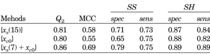
Table III compares results based on single or multiple feature vectors. The SVM classifier {xs(7)⫹ xc0} gives Q2⫽
86% and MCC⫽ 0.69, significantly improving on either {xs(15)} (Q2⫽ 81%) or {xc0} (Q2⫽ 80%). The combined SVM
classifier {xs(7) ⫹ xc0} considerably increases the MCC
value for bonded cysteines (from 0.58 or 0.55 to 0.69). Since {xc0} will fail in the case of proteins with mixed bonding
states of cysteines and {xs(15)} does not know of the global
“all-or-none rule” for bonded (or nonbonded) cysteines, a combination of local environment, xs(w), and global
proper-ties, xc0, can better capture essential features of cysteine
states.
Table IV lists the results obtained from SVMs coupled with CSS, which carries information about the global patterns of the cysteine states in proteins. When the SVM is coupled with CSS, we consistently obtain the overall prediction accuracy Q2ranging from 88% to 90%, and MCC
from 0.71 to 0.77. Just like a global property such as the amino acid composition, CSS can help significantly in-crease prediction accuracy. For example, {xs(15)} ⫹ CSS
yields prediction accuracy Q2⫽ 89%, about 8% higher than
that of {xs(15)}. In the case of {xs(7)⫹ xc0}, which includes
global property in terms of the amino acid compositions, the effects of CSS are not as pronounced as the previous example on increasing prediction accuracy (Q2from 86% to
88%). We also notice that the SVM⫹CSS significantly increases the specificity in predicting bonded cysteines ranging from 88% to 91%, compared with that of SVM based on local sequence windows (spec ⫽ 71% for SS). Combining multiple SVM classifiers coupled with CSS, we are able to obtain the best predictor: Q2⫽ 90% and MCC ⫽
0.77.
CONCLUSIONS
We have developed an approach to predict the bonding states of cysteine using SVM methods based on the local sequence windows and global descriptors such as the total amino acids and the cysteine state sequences. We found that the SVM method based on the combined local se-quence windows and global amino acid compositions signifi-cantly improves the predictive performances. Obviously, the combination of local environments of cysteines (such as local sequence windows) and global properties (such as total amino acid compositions) can better capture essential features of cysteine states. Coupled with CSS, SVM based on multiple-feature vectors yields 90% prediction accuracy and 0.77 MCC, considerably higher than the correspond-ing values 81% and 0.58, respectively, obtained by SVM based on local sequence windows. We also notice that the SVM⫹CSS significantly increases the specificity in predict-ing bonded cysteines (88 –91%), around 20% higher than that of SVM based on local sequence windows. Higher
TABLE I. Predictive Performance of SVM Based on Sequence Inputs of Different Window Lengths, {xs(w)} Window
length Q2 MCC
SS SH
spec sens spec sens
5 0.75 0.46 0.69 0.63 0.78 0.82 9 0.79 0.54 0.71 0.69 0.84 0.84 13 0.80 0.56 0.71 0.71 0.85 0.84 15 0.81 0.58 0.71 0.73 0.87 0.84 17 0.80 0.56 0.71 0.72 0.86 0.84 21 0.80 0.55 0.69 0.72 0.86 0.83
TABLE II. Predictive Performances of SVMs Based on Composition Inputs of Different Window Lengths, {xc(w)} Window
length Q2 MCC
SS SH
spec sens spec sens
9 0.67 0.22 0.29 0.59 0.88 0.69
15 0.70 0.31 0.41 0.62 0.87 0.73
25 0.73 0.38 0.46 0.67 0.89 0.75
35 0.75 0.42 0.51 0.69 0.89 0.76
Full length 0.80 0.55 0.65 0.75 0.88 0.82
TABLE III. Comparison of Predictive Performances of SVM Based on Single and Multiple Feature Vectors
Mehods Q2 MCC
SS SH
spec sens spec sens {xs(15)} 0.81 0.58 0.71 0.73 0.87 0.84
{xc0} 0.80 0.55 0.65 0.75 0.88 0.82
{xs(7)⫹ xc0} 0.86 0.69 0.79 0.75 0.89 0.89
TABLE IV. Comparison of Predictive Performances of SVMs Coupled with CSS
Methods Q2 MCC
SS SH
spec sens spec sens {xs(15)}⫹ CSS 0.89 0.74 0.91 0.74 0.87 0.97 {xs(7)⫹ xc0}⫹ CSS 0.88 0.71 0.88 0.74 0.87 0.95 {xs(7)⫹ xr(7)}⫹ CSS 0.88 0.73 0.89 0.74 0.87 0.95 Multiple SVM⫹ CSSa 0.90 0.77 0.91 0.77 0.89 0.97
aThe multiple SVM classifiers are { x
s(15)}, { xs(7)⫹ xc0}, and { xs(7)⫹
specificity in bonded cysteines allows for confident predic-tion and prevents error propagapredic-tions. Though we did not include structural information in our input vectors, it is possible to include structural information, such as the predicted secondary structures or the predicted solvent accessible areas of the cysteines, as well as the flanking residues in the windowing.
Our study shows that the bonding state of the cysteines is determined by both the local information of the particu-lar cysteine, such as the flanking amino acid sequences, and the global information, such as the composition con-tent of the proteins, as well as the bonding states of other cysteines. Our results may be useful in both protein modeling12,36 and protein engineering.37Recently, there
have been efforts to enhance the stability of proteins by introducing engineered disulfide bonds,38 – 40and our
re-sults may also be useful in suggesting appropriate resi-dues for disulfide crosslinking.
REFERENCES
1. Clark J, Fersht A. Engineered disulfide bonds as probes of the folding pathway of branase—increasing the stability of proteins against the rate of denaturation. Biochemistry 1993;32:4322– 4329.
2. Hwang J-K, Pan J-J. Classical trajectory mapping approach for simulations of classical reactions in solution and in enzymes. J Phys Chem 1996;100:909 –912.
3. Akamatsu Y, Ohno T, Hirota K, Kagoshima H, Yodoi J, Shigesada K. Redox regulation of the DNA binding activity in transcription factor PEBP2: the roles of two conserved cysteine residues. J Biol Chem 1997;272:14497–14500.
4. Abkevich VI, Shaknovich EI. What can disulfide bonds tell us about protein energetics, function and folding: simulations and bioinformatics analysis. J Mol Biol 2000;300:975–985.
5. Clarke J, Hounslow AH, Bond CJ, Fersht AR, Daggett V. The effects of disulfide bonds on the denatured state of barnase. Protein Sci 2000;9:2394 –2404.
6. Wedemeyer WJ, Welker E, Narayan M, Scheraga HA. Disulfide bonds and protein folding. Biochemistry 2000;39:4207– 4215. 7. Yokota A, Izutani K, Takai M, Kubo Y, Noda Y, Koumoto Y,
Tachibana H, Segawas S. The transition state in the folding-unfolding reaction of four species of three-disulfide variant of hen lysozyme: the role of each disulfide bridge. J Mol Biol 2000;295: 1275–1288.
8. Gladyshev VN. Thioredoxin and peptide methionine sulfoxide reductase: convergence of similar structure and function in dis-tinct structural folds. Proteins 2002;46:149 –152.
9. Anfinsen C, Scheraga HA. Experimental and theoretical aspects of protein folding. Adv Protein Chem 1975;29:205–300.
10. Vielle C, Zeikus G. Hyperthermophilic enzymes: sources, uses, and molecular mechanisms for thermostability. Microbiol Mol Biol Rev 2001;65:1– 43.
11. Hogg PJ. Disulfide bonds as switches for protein function. Trends Biochem Sci 2003;28:210 –214.
12. Chuang CC, Chen CY, Yang J-M, Lyu PC, Hwang J-K. Relation-ship between protein structures and disulfide-bonding patterns. Proteins 2003;53:1–5.
13. Muskal SM, Holbrook SR, Kim SH. Prediction of the disulfide-bonding state of cysteine in proteins. Protein Eng 1990;3:667– 672. 14. Fiser A, Cserzo M, Tudos E, Simon I. Different sequence environ-ments of cysteines and half cysteines in proteins: application to predict disulfide forming residues. FEBS Lett 1992;302:117–120. 15. Fiser A, Simon I. Predicting the oxidation state of cysteines by
multiple sequence alignment. Bioinformatics 2000;16:251–256. 16. Martelli PL, Fariselli P, Malaguti L, Casadio R. Prediction of the
disulfide bonding state of cysteines in proteins with hidden neural networks. Protein Eng 2002;15:951–953.
17. Muccielli-Giorgi MH, Hazout S, Tuffery P. Predicting the disulfide bonding state of cysteines using protein descriptors. Proteins 2002;46:243–249.
18. Fariselli P, Riccobelli P, Casadio R. Role of evolutionary informa-tion in predicting the disulfide-bonding state of cysteine in pro-teins. Proteins 1999;36:340 –346.
19. Martelli PL, Fariselli P, Malaguti L, Casadio R. Prediction of the disulfide-bonding state of cysteines in proteins at 88% accuracy. Protein Sci 2002;11:2735–2739.
20. Krogh A, Riis SK. Hidden neural networks. Neural Comput 1999;11:541–563.
21. Vapnik V. The nature of statistical learning theory. New York: Springer; 1995.
22. Jaakkola T, Kiekhans M, Haussler D. Using the Fisher kernel method to detect remote protein homologies. Intel Syst Mol Biol 1999;149 –158.
23. Brown MP, Grundy WN, Lin D, Cristianini N, Sugnet CW, Furey TS, Ares MJ, Haussler D. Knowledge-based analysis of microar-ray gene expression data by sing support vector machine. Proc Natl Acad Sci USA 2000;97:262–267.
24. Dingg CHQ, Dubchak I. Multi-class protein fold recognition using support vector machines and neural networks. Bioinformatics 2001;17:349 –358.
25. Hua S, Sun Z. A novel method of protein secondary structure prediction with high segment overlap measure: support vector machine approach. J Mol Biol 2001;308:397– 407.
26. Yu C-S, Wang J-Y, Yang J-M, Lyu PC, Lin C-J, Hwang J-K. Fine grained protein fold assignment by support vector machines using generalized n peptide coding schemes and jury voting from multiple-parameter sets. Proteins 2003;50:531–536.
27. Yu C-S, Lin C-J, Hwang J-K. Predicting subcellular localization of proteins for Gram-negative bacteria by support vector machines based on n-peptide composition. Protein Science 2004 (in press). 28. Schneider R, Sander C. Database of homology-derived structures
and the structural meaning of sequence alignment. Proteins 1991;9:56 –58.
29. Rost B, Sander C. Prediction of protein secondary structure at better than 70% accuracy. J Mol Biol 1993;232:584 –599. 30. Meiler J, Muller M, Zeidler A, Schmaschke F. Generation and
evaluation of dimension-reduced amino acid parameter represen-tations by artificial neural networks. J Mol Model 2001;7:360 – 369.
31. Berman HM, Westbrook J, Feng Z, Gilliland G, Bhat TN, Weissig H, Shindyalov IN, Bourne PE. The Protein Data Bank. Nucleic Acids Res 2000;28:235–242.
32. Durbin R, Eddy SR, Krogh A, Mitchison G. Biological sequence analysis. New York: Cambridge University Press; 1998.
33. Chang C-C, Lin C-J. LIBSVM: a library for support vector machines. 2001. Software available from http://www.csie.ntu. edu.tw/⬃cjlin/libsvm.
34. Saitou N, Nei M. The neighbor-joining method: a new method for reconstructing phylogenetic trees. Mol Biol Evol 1987;4:406 – 425. 35. Matthews BW. Comparison of the predicted and observed second-ary structure of T4 phage lysozyme. Biochim Biophys Acta 1975;405:442– 451.
36. Harrison PM, Sternberg MJE. The disulfide beta-cross: from cystine geometry and clustering to classification of small disulfide-rich protein folds. J Mol Biol 1996;264:603– 623.
37. Yokota A, Izutani K, Takai M, Kubo Y, Koumoto Y, Tachibana H, Segawa S. The transition state in the folding-unfolding reaction of four species of three-disulfide variant of hen lysozyme: the role of each disulfide bridge. J Mol Biol 2000;295:1275–1288.
38. Hinck AP, Truckses Dm, Markley JL. Engineered disulfide bonds in staphylococcal nuclease: effects on the stability and conforma-tion of the folded protein. Biochemistry 1996;35:10328 –10338. 39. Mansfeld J, Vriend G, Dijkstra BW, Veltman OR, Van den Burg B,
Venema G, Ulbrich-Hoffmann R, Eijsink VG. Extreme stabiliza-tion of a thermolysin-like protease by an engineered disulfide bond. J Biol Chem 1997;272:11152–11156.
40. Shimaoka M, Lu C, Salas A, Xiao T, Takagi J, Springer TA. Stabilizing the integrin alpha M inserted domain in alternative conformations with a range of engineered disulfide bonds. Proc Natl Acad Sci USA 2002;99:16737–16741.