含水層參數檢定與洩降敏感度分析

國 立 交 通 大 學

環 境 工 程 研 究 所

博

士 論 文

含水層參數檢定與洩降敏感度分析

Aquifer Parameter Estimation and

Drawdown Sensitivity Analysis

研

究 生：黃彥禎

指 導 教 授 ： 葉 弘 德

含水層參數檢定與洩降敏感度分析

Aquifer Parameter Estimation and

Drawdown Sensitivity Analysis

研 究 生 ： 黃彥禎 Student：Yen-Chen Huang

指導教授：葉弘德 Advisor：Hund-Der Yeh

國 立 交 通 大 學

環 境 工 程 研 究 所

博 士 論 文

A Dissertation

Submitted to Institute of Environmental Engineering College of Engineering

National Chiao Tung University for the Degree of

Doctor of Philosophy In Environmental Engineering

November, 2007 Hsinchu, Taiwan

含水層參數檢定與洩降敏感度分析

研究生：黃彥禎 指導教授：葉弘德 國立交通大學 環境工程研究所

中文摘要

抽水試驗是調查含水層水文地質參數的重要方法，傳統的分析方式，都應用圖解法 或數值方法中的梯度法求解，然而，這些方法都有其限制。本研究建立一參數檢定模式， 應用模擬退火演算法結合水層抽水洩降的解析模式，推求滲漏及自由含水層的參數。結 果顯示此參數檢定模式較傳統圖解法，更能準確求出水層參數值，且與擴展式卡門濾波 和牛頓法的結果精度相同。此外，本研究對模擬退火演算法的控制參數進行敏感度分 析，結果顯示本方法是可信賴、且穩定的。 一般而言，進行一個抽水試驗需要花費許多人力及資源，包括井的設置、數據的量 測及分析等。若洩降數據不足，使用傳統圖解分析方法，往往無法得到正確的答案。長 時抽水及人力需求的問題，可透過於現地量測洩降數據的同時，即時檢定含水層的參 數。然而，在滲漏及自由水層部分的水文地質特性，需要抽水一段時間後，才會充分的

的時間。本研究使用敏感度分析，尋找滲漏與自由水層的參數，在進行抽水試驗時，反 應於洩降的影響時程。同時，應用建立的參數檢定模式，即時推求參數值。結果顯示當 含水層參數開始影響洩降時，即時參數檢定模式立刻正確的檢定出水層參數值。這個發 現可作為停止參數檢定時間的重要參考。此外，本研究透過敏感度分析，進一步分析、 探討不同的比出水率，及不同的抽水井與觀測井間的距離，對於試驗停止時間的影響。 關鍵字：地下水、抽水試驗、參數檢定模式、模擬退火演算法、即時檢定、敏感度分析、 滲漏含水層、自由含水層

Aquifer Parameter Estimation and Drawdown Sensitivity Analysis

Student: Yen-Chen Huang Advisor: Dr. Hund-Der Yeh

Institute of Environmental Engineering National Chiao Tung University

ABSTRACT

The pumping test is a very important method in investigating the aquifer hydrogeologic characteristics. Conventional graphical or computer methods for identifying aquifer parameters have their own inevitable limitations. This study applies the parameter estimation model (PEM) based on the simulated annealing (SA) and analytical models to estimate the parameters of leaky and unconfined aquifers. The estimated results of proposed method have better accuracy than those of the graphical methods and agree well with those of the computer methods based on the extended Kalman filter and Newton’s method. Moreover, the sensitivity analyses for the control parameters of SA indicate that the proposed method is very robust and stable in parameter estimation procedures.

estimated aquifer parameters obtained from graphical approaches may not be in good accuracy if the pumping time is too short to give a good visual fit to the type curves. The problems of long pumping time and required efforts can be reduced if the drawdown data are measured and the parameters are simultaneously estimated on-line. However, the drawdown behavior of the leaky and unconfined aquifers in response to the pumping may have a time lag. The time to terminate the estimation may not be easily and quickly to decide when applying a PEM on-line to analyze the parameters. This study employs the sensitivity analysis to analyze the influence period of parameters in response to the pumping in both leaky and unconfined aquifers. In the meanwhile, a PEM based on the SA is used to determine the parameters of these two aquifers on-line. The results indicate that the aquifer parameters can be accurately estimated when they start to influence the drawdown. This finding can be used as a guide in terminating the estimation. Moreover, the sensitivity analysis is also used to study the effects of different values of specific yield Sy and the distance between pumping

well and observation well on the influence time of Sy during the pumping.

Key Words: Groundwater; Pumping test; Parameter estimation model; simulated annealing; on-line estimation; sensitivity analysis; leaky aquifer; unconfined aquifer

誌謝

本論文承蒙葉弘德教授細心指導與鼓勵，才得以順利完成，在此表示最誠摯的謝 意。口試期間，台灣大學劉振宇教授、徐年盛教授；中國科技大學陳主惠教授；中央大 學吳瑞賢教授；及交通大學張良正教授，對本論文之疏漏的指正與對內容的精闢見解， 使本論文更加充實完備，於此一併致謝。 在攻讀博士的修業生涯中，葉弘德教授不但將專業知識傾囊相授，其認真嚴謹的治 學態度，與充分享受生命的生活方式，都使我受益良多。另外，由衷的感謝研究室的夥 伴們：紹洋、智澤、郁仲、子鈞、彬原、雅琪、易哲、君豪、彥如、桐樺、淇汾、易璁、 敏筠、毓婷、士賓、和博傑等，在學業上的切磋砥礪，與生活上的互相幫助。最後，感 謝家人、親愛的老婆俐伶、及寶貝女兒予星對我的全力支持與愛護，願將本論文獻給你 們。

TABLE OF CONTENTS

中文摘要... I ABSTRACT ... III

誌謝... V TABLE OF CONTENTS ... VI LIST OF TABLES ... VIII LIST OF FIGURES... IX NOTATIONS... X

CHAPTER 1 INTRODUCTION...1

1.1 Background...1

1.2 Objectives ...4

CHAPTER 2 LITERATURE REVIEW...7

2.1 Theoretical Development and Analysis...7

2.2 Simulated Annealing ...10

2.3 Sensitivity Analysis ... 11

CHAPTER 3 METHODOLOGY ...14

3.1 Analytical Models of Leaky and Unconfined Aquifers ...14

3.2 Simulated Annealing Algorithm ...18

3.3 Integration of the SA with Analytical Models...21

3.4 Sensitivity Analysis ...22

3.5 Assessment for Estimated Errors...23

CHAPTER 4 RESULTS AND DISCUSSION...25

4.1 Parameter Estimation Using the PEM Based on the SA ...25

4.1.1 Estimation of leaky aquifer parameters ...25

4.1.2 Estimation of unconfined aquifer parameters...27

4.1.3 The sensitivity analysis of SA’s control parameters ...28

4.2 Sensitivity Analysis of Aquifer Parameters...29

4.3 Parameter Estimation using On-line PEM ...33

CHAPTER 5 CONCLUSIONS ...41

REFERENCES ...44

VITA (個人簡歷) ...79

LIST OF TABLES

Table 1 Time-drawdown data of three observations wells [Cooper, 1963, p. 31]...49

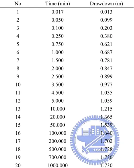
Table 2 Time-drawdown data [Sridharan, 1987, p. 170] ...50

Table 3 Comparison of results from three-parameter model when using SA, EKF, and NLN to analyze Cooper’s data [Cooper, 1963] ...51

Table 4 The estimated parameters and estimated errors when using SA, EKF, and NLN to analyze Sridharan’s data [Sridharan et al., 1987] ...52

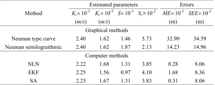
Table 5 Comparison of results when applying graphical methods, NLN, EKF, and SA methods to analyze the pumping test data obtained from an unconfined aquifer...53

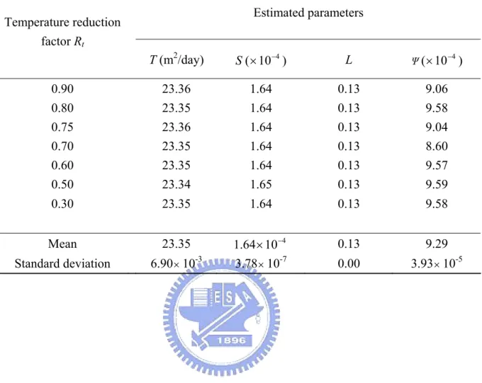
Table 6 Estimated parameters using different temperature reduction factor...54

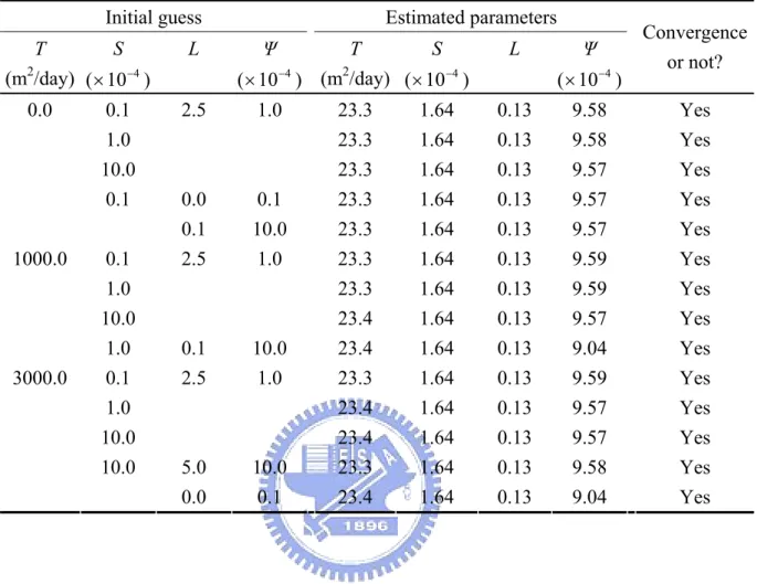
Table 7 Comparison of the results in leaky aquifer considering storage effect when using different initial guesses...55

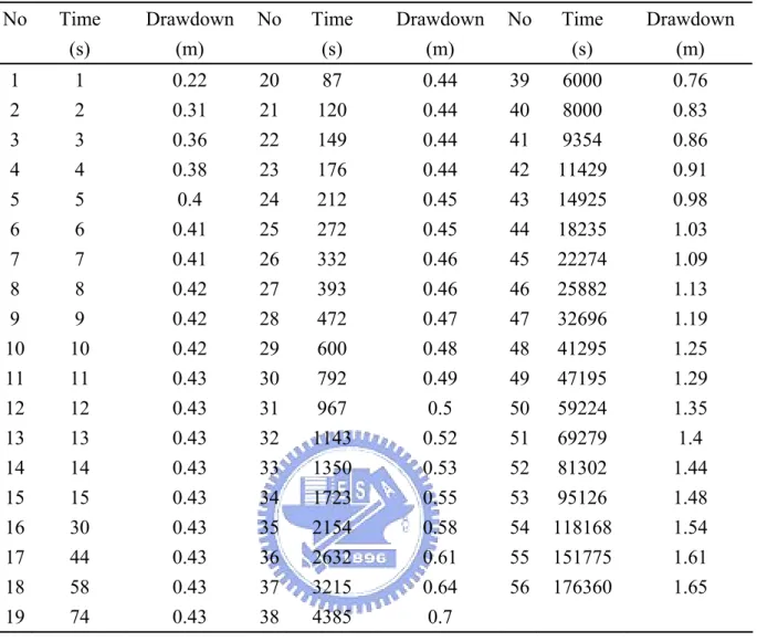
Table 8 The synthetic drawdown data for the leaky aquifer...56

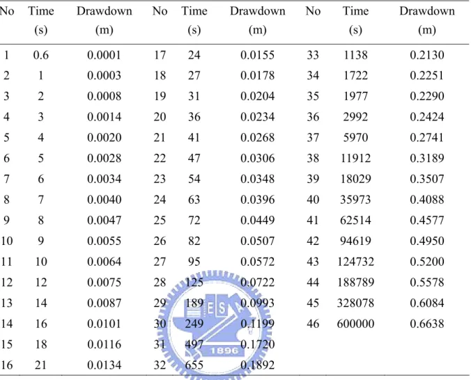
Table 9 The synthetic drawdown data set 1 for the unconfined aquifer...57

Table 10 The synthetic drawdown data set 2 for the unconfined aquifer...58

Table 11 Number of observations used in the synthetic data analysis and the estimated parameters for a leaky aquifer ...59

Table 12 The field time-drawdown data and the estimated parameters for a leaky aquifer using different number of observations...60

Table 13 Number of observations used in the data analysis and the estimated parameters based on the synthetic data set 1...61

Table 14 Number of observations used in the data analysis and the estimated parameters based on the synthetic data set 2...62

Table 15 The estimated parameters for an unconfined aquifer (Cape Cod site) using different number of observations ...63

LIST OF FIGURES

Figure 1 The sketch of the pumping tests of (a) leaky aquifer and (b) unconfined aquifer ...64

Figure 2 Flowchart of the SA ...65

Figure 3 The flowchart of the identification procedure (a) conventional method, (b) present method ...66

Figure 4 The estimated drawdowns and the pumping test data for the observation wells in the leaky aquifer without considering storage effect...67

Figure 5 The estimated drawdowns and the pumping test data for the observation wells in the leaky aquifer with considering storage effect...68

Figure 6 The estimated drawdown and the pumping test data obtained from an unconfined aquifer using SA ...69

Figure 7 The time-drawdown data and the normalized sensitivities of the leaky aquifer parameters...70

Figure 8 The time-drawdown data and the normalized sensitivities of the unconfined aquifer parameters (Neuman’s model)...71

Figure 9 The normalized sensitivities of the unconfined aquifer parameters (Moench’s model) ...72

Figure 10 The estimated L versus time in the leaky aquifer case...73

Figure 11 The estimated Sy versus time using the synthetic data set 1...74

Figure 12 The estimated Sy versus time using the synthetic data set 2...75

Figure 13 The estimated Sy versus time in the field unconfined aquifer ...76

Figure 14 The normalized sensitivity of Sy for Sy = 0.01, 0.1, or 0.3 and r = 10 m ...77

NOTATIONS

b : thickness of aquifer (L)

'

b : thickness of aquitard (L)

B : leakage factor, Tb' K' (L)

D : random number between zero and one

D1 : random number between zero and one

D

d : dimensionless vertical distance between the top of perforation in the pumping well and the initial position of water table, d /b

E : the system energy

( )

x

f : objective function

( )

0

J : zero order Bessel function of the first kind

K : hydraulic conductivity of main aquifer (LT-1)

k : Boltzmann’s constant '

K : vertical hydraulic conductivity of leaky confining layer (LT-1)

Kr : horizontal hydraulic conductivity of unconfined aquifer Kz : vertical hydraulic conductivity of unconfined aquifer

L : leakage coefficient, r B

D

l : dimensionless vertical distance between the bottom of perforation in the pumping well and the initial position of water table, l /b

ME : mean error between estimated drawdowns and pumping test data

n : total number of the time step

i

h

O : observed drawdowns at time step i

Pi : ith input parameter of the system

i

h

P : estimated drawdowns at time step i

P(E) : occurrence probability

PSA : acceptance probability

Q : the discharge of the well (L3T-1)

r : radial distant from pumping well (L)

Rt : temperature reduction factor

rw : outside radius of the pumped well screen S : storage coefficient the aquifer

'

S : storage coefficient of the aquitard

s : drawdown t i S_{, : normalized sensitivity} pi S _{: parametric sensitivity} Ss : specific storage

Sy : specific yield of unconfined aquifer

SEE : standard error of estimate for the estimated drawdowns

T : transmissivity (L2T-1)

Te : temperature of the system

s

t _{: Tt/Sr}2

D

t : dimensionless time for pumping aquifer, t_{D =}Tt r2S

D

t : _{t L}2 _16ψ2

D

u _{: dimensionless parameter, r}2_{S 4Tt} VM : step length vector

i

(

u r B

)

W , : leaky well function without considering the storage effect in aquitard

i

x _{: corresponding to zero of the n order Laguerre polynomials} th D

z : dimensionless elevation of observation point

,

z/b

β : _{K r}2_{/K b}2

r

z in unconfined aquifer system

β : r S' S/4B in leaky aquifer system σ : S /S_y

CHAPTER 1 INTRODUCTION

1.1 Background

Groundwater is an important source of water supply for drinking, agriculture, and industry. It represents 98% of freshwater readily available to humans [Schwartz and Zhang, 2002]. Groundwater is found in aquifers, which have the capability of both storing and transmitting groundwater. Recently, the groundwater problems, such as industrial wastewater injected into groundwater system and seawater intrusion, have been attracted public attention. The hydraulic properties of the aquifer systems have to be determined prior to characterizing or investigating the pollutant and its plume. Groundwater hydrologists often conduct aquifer tests to determine the in situ hydraulic properties of the soil formation, such as hydraulic conductivity and storage coefficient. These parameters are necessary information for quantitative and/or qualitative groundwater studies.

The pumping test is a very reliable method for estimating aquifer parameters. Figures 1 (a) and (b) display the sketch of the pumping tests in leaky and unconfined aquifers, respectively. Typically, a pumping test consists of a pumping well and one or more observation wells. The observation wells are located at varying distances from the pumping

pumping. The term drawdown (s in Figures 1 (a) and (b)) shows the change in water levels

through the test. The drawdown curve which describes a conical shape is cone of depression.

In the past, the pumping test data was usually analyzed using a graphical procedure with type curves to estimate the aquifer parameters. In addition, the parameters can also be obtained by computer methods, which usually estimate parameters using the least-square approach by taking the derivative of the sum of square errors between the observed and estimated drawdowns with respect to the parameters. The gradient-type methods are then utilized to solve the nonlinear least-square equations to determine the best-fit parameters. However, two disadvantages might be occurred when the gradient-type methods were used to solve the nonlinear least-square equations to obtain the parameters. First, those methods may yield divergent results if the initial guesses of parameters are not close enough to the target parameter values. Second, those methods may give poor results if improper increments were made when applying finite difference formula to approximate the derivative terms appeared in the least-square equations.

Recently, the computer-based parameter estimation models (PEM) were developed promptly. The models of aquifer parameter estimation usually combine a suitable solution for describing the pumping test with an optimization approach such as simulated annealing (SA) or a recursive approach, such as extended Kalman filter (EKF). Some commercial

softwares, like AQTESOLV [Duffield, 2002], use nonlinear weighted least-squares approach to fit the time-displacement data obtained from an aquifer test to the type curve.

A pumping test was usually required to perform for a long period of time if a graphical approach is chosen to analyze the measurement data. Otherwise, the estimated result may not be in good accuracy if the data is too short and the data points are too sparse to give a good visual fit to the type curve. However, such a test would spend a lot of time, money, and groundwater resources. These problems were aggravated when analyzing the data from the leaky and unconfined aquifers.

In a leaky aquifer, the semi-pervious bed (also shown as the aquitard in Figure 1 (a)), although of very low permeability, may yield significant amounts of water to the adjacent pumped aquifer. As time increased, leakage across the semi-pervious bed may become appreciable and flow is not restricted to the pumped aquifer alone. The additional water may be derived from storage of the aquitard and adjacent unpumped aquifers. During the pumping, the water is immediately withdrawn from the aquifer and then the head difference between two aquifers induces a flow across the aquitard. Therefore, the parameters of the confining bed (aquitard) may not be accurately estimated if only first few drawdown data points are used. Two approaches have been developed for dealing with leaky aquifers, one considers the aquitard storage while the other does not consider.

[Charbeneau, 2000]. In the first stage, water is immediately released from storage due to the compaction of the aquifer and the expansion of the water. In the second stage, the vertical gradient near the water table causes drainage of the porous matrix. The vertical hydraulic conductivity Kz begins to contribute to the pumping and the rate of descent in the hydraulic

head slows or stops after a period of time. Finally, the flow is horizontal and most of the pumping is supplied by the specific yield, Sy. Therefore, the analysis of Sy requires sufficient

long drawdown data fallen at the third section. In some cases, the effect of well bore storage needs to be considered since the diameter of pumping well is large. The water is withdrawn first from the casing at the beginning of pumping. Then the groundwater flow into the well because the head difference between the well and the adjacent formation.

Most physical systems can be viewed as input-output models that relate the output information to the proper input parameters. Unfortunately, the input parameters can not be known perfectly in the real world. Hence, the basic concept of sensitivity analysis is to investigate how the errors in the input parameters influence the outputs, or, in particular, to study if a small perturbation in the input parameters causes a large change in the output. Now the sensitivity analysis is being wildly applied in all sciences.

1.2 Objectives

First part:

(1) To develop a PEM based on the SA combined with Hantush and Jacob’s model [1955] or Neuman and Witherspoon’s model [1969] to estimate the parameters of leaky aquifer with or without considering the aquitard storage in the field;

(2) To propose a PEM based on SA coupled with the Neuman’s model [1975] for unconfined aquifers to automatically determine the best-fit aquifer parameters.

(3) To test the robustness and stability of the SA with different control parameters;

In the first part, three sets of field pumping test data are chosen, two for the leaky aquifer and one for the unconfined aquifer. The first one is reported in Cooper [1963], the second is select from Sridharan et al. [1987], and the last is obtained from Batu [1998].

Second part:

(1) To investigate the influence period of leaky and unconfined parameters using sensitivity analyses;

(2) To apply a PEM based on SA algorithm to on-line estimate the parameters in both leaky and unconfined aquifers using the synthetic and real field time-drawdown data sets;

(3) To employ the software AQTESOLV to estimate the parameters of unconfined aquifer with considering the effect of well bore storage using the synthetic data set;

applying the on-line PEM in determining the aquifer parameters;

(5) To study the influence period of the Sy in the cases of different Sy values and different

distance between pumping well and observation well via sensitivity analysis.

In the second part, three synthetic drawdown data sets, one for leaky aquifer (generated based on Hantush and Jacob’s model, 1955), and two for unconfined aquifer (generated based on Neuman’s model, 1974; and Moench’s model, 1997), are analyzed using the sensitivity analysis and on-line PEM. Moreover, the field data set of an unconfined aquifer obtained from Cape Cod, Massachusetts [Moench et al., 2000] is also analyzed by on-line PEM.

CHAPTER 2 LITERATURE REVIEW

2.1 Theoretical Development and Analysis

Hantush and Jacob [1955] described a mathematical model for non-steady radial flow to a well in a fully penetrated leaky aquifer under a constant pumping rate. In this model, the aquitard is overlain by an unconfined aquifer, and the main aquifer is underlain by an impermeable bed. Their analytical solution for the mathematical model is referred to as the three-parameter model in this dissertation. Hantush [1960] also presented a modified approach to include the effect of the aquitard storage. Neuman and Witherspoon [1969] gave a model describing the drawdown of the lower and pumped aquifer in a hydrogeologic system which is composed of two confined aquifers and one aquitard. Their solution, which considers the effect of aquitard storage and neglects the drawdown in the unpumped aquifer, is called the four-parameter model. Both the three-parameter and four-parameter models are also mentioned in several books, for example, Dawson and Istok [1991] and Batu [1998]. In the three-parameter model, the graphical method based on Hantush’s or Walton’s type curves [Batu 1998] requires data plotting work and individual judgment during the curve fitting procedure. Therefore, errors may be introduced during the fitting process. In the four-parameter model, the use of the graphical matching method based on the Neuman and

Witherspoon’s model is practically impossible since there will be several families of type curves.

Boulton [1954, 1963] developed an analytical solution by introducing the concept of delayed yield for unconfined formations. Prickett [1965] presented a systematic approach to estimate the parameters using a graphical procedure based on Boulton’s type curves. Cooley and Case [1973] displayed that Boulton’s equation yields an exact solution where it describes a flow system with a rigid phreatic aquitard on top of the main aquifer, and the unsaturated flow above the water surface is neglected. Neuman [1972, 1974] developed a solution that considers the effects of elastic storage and anisotropy of aquifers on drawdown behavior. Neuman’s model treated the unconfined aquifer as a compressible system and the water surface as a moving boundary. His theory was also extended to account for the effect of a partially penetrating pumping well or/and an observation well in a homogeneous anisotropic unconfined aquifer. Neuman [1975] also gave a graphical type curve solution process to estimate the aquifer parameters. Moench [1995] combined the Boulton and Neuman models for flow toward a well in an unconfined aquifer. McElwee [1980] proposed a least-squares fitting technique and sensitivity analysis to analyze the time-drawdown data for the aquifer parameters. Saleem [1970] proposed a nonlinear programming technique, minimizing the sum of squares of the differences between observed and estimated drawdowns. Mania and Sucche [1978] employed the least-squares approach to analyze parameters in unconfined

aquifers, based on Boulton's solution for large-time data. Sridharan et al. [1985] used sensitivity analysis technique based on Neuman's model for the condition of a fully penetrating well for identifying parameters in an unconfined aquifer. Yeh [1987] employed the nonlinear least-squares and finite-difference Newton’s method (NLN) for estimating the parameters of the confined aquifer. Yeh and Han [1989] subsequently applied NLN to determine the parameters of the leaky aquifers. Huang [1996] used NLN to identify the unconfined aquifer parameters. The NLN approach has the advantage of high accuracy and quick convergence for reasonable initial guesses. However, those methods may yield divergent results if the initial guess parameter values are not close enough to the target values. In addition, they may obtain poor results if improper increments were made when applying finite difference formula to approximate the derivative terms appeared in the least-square equations. Recently, the Kalman filter has been successfully applied to the aquifer parameter and water table related estimations. Chander et al. [1981] estimated the parameters for both nonleaky and leaky aquifers by the iterated extended Kalman filter. Leng and Yeh [2003] employed EKF to identify the aquifer parameters in confined and unconfined aquifer systems. Yeh and Huang [2005] utilized the EKF to estimate the aquifer parameters in leaky aquifer systems with and without considering the storage effect in the aquitard. The results indicate that the EKF can be applied to analyze the measurement drawdown data even with white noise or temporally correlated noise.

2.2 Simulated Annealing

The theory of SA was developed by Metropolis et al. [1953]. They introduced a simple algorithm to incorporate the idea of the behavior of a particle system in thermal equilibrium into numerical calculations of an equation state. SA is a random search algorithm that allows, at least in theory or in probability, to obtain the global optimum of a function in any given domain. SA is an evolution from descent search method. The major difference between SA and conventional descent method is that the SA used Metropolis mechanism, or called the Boltzmann’s mechanism, to control which ascent moves could be accepted. In other words, the SA uses descent strategy but allows random ascent moves to avoid possible trap in a local optimum. This property prevents the SA from having the same problem as those of the descent method. SA was successfully applied in wide range of optimization applications. Kirkpatrick et al. [1983] applied it to solve large-scale combinatorial optimization problems. Goffe et al. [1994] employed SA to solve four econometric problems and compared the results obtained from the conventional algorithms. Their solutions obtained from SA were superior to those obtained from the conventional algorithm. Subsequently, utilization of SA in optimization problems has been applied in hydrological engineering. Dougherty and Marryott [1991] and Marryott et al. [1993] employed the SA to design the strategies of groundwater remediation. Zheng and Wang [1996] used the tabu search and SA to estimate the parameter structure using preliminary results from

one-dimensional examples. Cunha and Sousa [1999] used SA to minimize the capacity extension cost of the water distribution network. The solution set obtained from SA and nonlinear programming (NLP) techniques for several medium size networks showed that SA did provide a better solution in general, in comparison with that obtained by the NLP techniques. Kuo et al. [2001] applied SA to agricultural water resource planning and management. Tsai et al. [2003] developed two global-local optimization methods for identifying the parameter structure in groundwater modeling. Tung et al. [2003] developed an optimal zoning procedure by applying simulated annealing (SA) and the shortest distance method with MODFLOW to determine the best zonation of hydraulic conductivity. Lin and Yeh [2005] employed SA to predict the concentrations of trihalomethane (THM) species in a water distribution system. Chang et al. [2007] used SA to give an approximate result for a two-dimensional problem if decomposing the model area into a number of transects along the transverse direction, estimating the parameter values along the longitudinal direction for each transect, and then smoothing the estimated results.

2.3 Sensitivity Analysis

Cukier et al. [1973, 1975, and 1978] as well as Schibly and Shuler [1973] developed a statistical approach for sensitivity analysis to nonlinear algebraic equations. Kabala and Milly [1990] used sensitivity analysis for analyzing the effect of parameter uncertainty and

soil heterogeneity on the transport of moisture in unsaturated porous media. Jiao and Rushton [1995] provided a sensitivity analysis of drawdown to parameters and its influence on parameter estimation for pumping tests in large-diameter wells. They concluded that the well storage reduces the sensitivities of drawdown to transmissivity and storativity, and increases the correlation between them. This leads to uncertainties in estimating the aquifer parameters, especially storativity. Kabala [2001] reviewed the basic concepts of sensitivity analysis and pointed out their limitations. He used logarithmic sensitivity to a model of a pumping test conducted on a fully penetrating well that accounting for the wellbore storage and an infinitesimal skin in a confined aquifer. The results demonstrated that transient flowmeter test measurements of drawdown and wellface flow rate should not be made during the early times of the wellbore storage phase. Shih et al. [2002] provided an analytical solution and sensitivity analysis to study the contaminant transport in fractured media considering pulse, Dirac delta and sinusoid input source. Kabala et al. [2002] also studied the logarithmic sensitivity, plausible relative errors, and deterministic parameter correlations in a simple semi-analytic no-crossflow model of the transient flowmeter test (TFMT) that accounts for a thick skin around the wall. Vachaud and Chen [2002] analyzed a large-scale hydrologic model problem by sensitivity theory. The results indicated that different levels of simplification of the input data can be selected depending on the objectives of the modeling and the level of acceptable losses of information on outputs. Ochs et al. [2003] used

sensitivity analysis to study the radionuclide migration in compacted bentonite. The results indicated that the changes in radionuclide solution speciation leaded to different diffusing species under different conditions and the effects on diffusion through changes in the electric double layer properties of the clay pores was a function of ionic strength. Gooseff et al. [2005] performed sensitivity analysis of a conservative transient storage model and two different reactive solute transport models. The results showed that the reactive solute simulations appear to be most sensitive to data collected during the rising and falling limb of the concentration breakthrough curve.

CHAPTER 3 METHODOLOGY

3.1 Analytical Models of Leaky and Unconfined Aquifers

Leaky aquifer:

The analytical model without considering the storage effect in aquitard

Hantush and Jacob’s model (three-parameter model in this study) describing the drawdown within a leaky aquifer in response to the pumping as a function of radial distance and time. The drawdown s is shown as [Batu, 1998; Hantush and Jacob, 1955]

⎟ ⎠ ⎞ ⎜ ⎝ ⎛ ⋅ = B r u W T Q s , 4π (3.1.1)

where T is transmissivity, B is the leakage factor and is defined as

(

K' b'

)

T , K ′ is the

vertical conductivity of a leaky confining bed, b′ is thickness of aquitard, r B = L is

named as leakage coefficient, r is the distance between pumping well and observation well, u

is the dimensionless variable and is defined as r2S 4Tt_{, S is storage coefficient, W(u, r/B) is}

the leaky well function, and Q is the pumping rate. Note that the typical values of T, S, and L range from zero to 3000 (m2/day), 10-3 to 10-5, and zero to 5, respectively. The leaky well function W (u, r/B) may be expressed as

(

)

∫

∞ _⎥⋅ ⎦ ⎤ ⎢ ⎣ ⎡ − − ⋅ = ⎟ ⎠ ⎞ ⎜ ⎝ ⎛ u y dy B r y y B r u W 4 / exp 1 , 2 (3.1.2)

numerical approach is required to evaluate the integration. Both the Laguerre quadrature formula and Gaussian quadrature formula [Carnahan et al., 1969] are employed to evaluate

the values of leaky well function with the accuracy to the fourth decimal. The Laguerre integration used to approximate an integral function is usually expressed as

( )

_∑

( )

∫

∞ _⋅ − _{= =}n _⋅ i i i x_{dx w f x} e x f 1 0 (3.1.3)

where the w is weighting factor and _i x is corresponding to zero of the nth order Laguerre _i

polynomials. For a small value of u, the Laguerre quadrature formula can not give the desired accuracy. Therefore the Gaussian quadrature formula is employed to evaluate the integration of Eq. (3.1.2) when u is small.

The analytical model with storage effect in aquitard:

Neuman and Witherspoon developed a closed-form solution (four-parameter model in this study) for the problem of flow to a well in a confined infinite radial system composed of two confined aquifers that are separated by an aquitard [Neuman and Witherspoon, 1969]. Differing from Hantush and Jacob’s work [1955], Neuman and Witherspoon’s model includes the effect of the aquitard storage on the drawdown of the pumping aquifer. Their model may be written as

(

)

[

y t

]

J

[

w

( )

y

]

dy y T Q s =

_∫

∞ − − _D ⋅ ₀ ⋅ 0 2 exp 1 1 2

π

(3.1.4) where _{t =t L}2 _16ψ2 _{, t =Tt r}2_{S , L=r B , ψ =β L , B= Tb' K′ ,}

S B S

r ' 4

=

β , S' is the storage coefficient of the aquitard, and

( )

y L y L y y

w2 ₌ 2 2 16_ψ2 ₋ 2_{⋅ ⋅}cot _{. Note that Eq. (3.1.4) is valid for all values of time} intervals and the Bessel function of the first kind J₀

[

w

( )

y

]

must be set to zero when

( )

0

2 _{y <}

w .

Unconfined aquifer:

The analytical model without considering well-bore storage effect

The solution for the equation describing the groundwater flow system in an unconfined aquifer developed by Neuman [1974] is

dy y u y u y yJ T Q t z r s n n

∫

∞

∑

∞ = ⎥⎦ ⎤ ⎢ ⎣ ⎡ ₊ = 0 1 0 2 / 1 0( ) ( ) ( ) 4 4 ) , , ( β π (3.1.5)

where z denotes the elevation of observation point, J₀(x)is the zero order Bessel function of the first kind, _{K r}2 _{/K b}2

r z

=

β is a dimensionless parameter, Kr is radial hydraulic

conductivity, Kz is vertical hydraulic conductivity, y is a dummy variable, and

) sinh( ) ( )] 1 ( sinh[ )] 1 ( sinh[ ) cosh( ] / ) ( ) 1 ( [ ) cosh( )]} ( exp[ 1 { ) ( 0 0 0 0 2 2 0 2 2 0 2 0 2 0 2 0 r d l l r d r r r y r y z r r y t y u D D D D D s − − − − ⋅ − − + + − − − = σ σ β (3.1.6) ) sin( ) ( )] 1 ( sin[ )] 1 ( sin[ ) cos( ] / ) ( ) 1 ( [ ) cos( )]} ( exp[ 1 { ) ( _{2 2 2 2 2} 2 2 n D D D n D n n n n D n n s n r d l l r d r r r y r y z r r y t y u − − − − ⋅ + − + − + − − = σ σ β (3.1.7) where _{t Tt/Sr}2

s = represents the dimensionless time since pumping started, Ss is the specific

the thickness of the aquifer, σ =S /S_y is a dimensionless parameter, Sy is specific yield,

b d

d_D = / denotes the dimensionless vertical distance between the top of perforation in the pumping well and the initial position of water table, and l_D =l/b is the dimensionless vertical distance between the bottom of perforation in the pumping well and the initial position of water table. The term of r and ₀ r are respectively the roots of the following _n

two equations 0 ) cosh( ) ( ) sinh( 2 ₀ 0 2 0 0 r − y −r r = r σ , 2 2 0 y r < (3.1.8) and 0 ) cos( ) ( ) sin( ₊ 2 ₊ 2 ₌ n n n n r y r r r σ , (2n−1)(π /2)<r_n <nπ

(3.1.9)

The analytical model with well-bore storage effect

Moench [1997] derived a Laplace domain solution for unsteady flow to a partially penetrating large-diameter well in an unconfined aquifer. The dimensionless drawdown in Laplace domain is

(

)

₍

₎

_[

₍

₎

_]

w D D D D D D S A pW d l p E p z r h + + − = 1 2 , , (3.1.10) where

(

)

∑

( )

{

[

( )

(

[

)

]

[

( )

(

]

)

]

}

∞ = + − − − − = 0 1 2 0 2 sin 5 . 0 1 sin 1 sin 2 n n n n n n D n D n n D D q K q l d q K d l A ε ε ε ε ε (3.1.11)

(

) (

)

[

(

(

)

)

(

(

)

)

]

( )

[

( )

]

∑

∞ = + − − − = 0 1 0 2 sin 5 . 0 1 sin 1 sin cos 2 n n n n n D n D n D n D n q K q l d z r q K E ε ε ε ε ε (3.1.12)

(

l d

)

S r r W_D = _c2 _w2 _s − 2π π , q_n =

(

ε_n2β_w + p

)

_,

(

2 2

)

D n D nr pr q = ε β + , _{βw =}r_w2K_z b2K_{r ,} 2 2 _{/K b} r K_{z r} =

β , S_w =K_rd_s K_sr_w , and r_D =r/r_w. The rw and rc represent the outside

radius of the pumped well screen and casing, respectively. The symbol ε_n is the root of

( ) (

ε σβ γ

)

ε p p w n n tan = ₊ (3.1.13)

where σ =S S_y , γ =α₁bS_y K_z , and α is a fitting parameter for drainage from the ₁ unsaturated zone and has units of inverse time (1/T). A large value of α₁ effectively eliminates the effect of this parameter from the solution. The Stefest method is used for the numerical Laplace inversion.

3.2 Simulated Annealing Algorithm

The basic algorithm of simulated annealing is motivated by an analogy to the thermodynamics of annealing in solids, such as growing silicon in the form of highly ordered, defect-free crystals. In order to accomplish this, the material is annealed. It is first heated to a temperature that allows many molecules to move freely with respect to each other. After that, it is cooled slowly until the material freezes into a crystal, which is completely ordered, and thus the system is at the state of minimum energy. In other words, the molecules have high activity when the temperature is high and the crystalline configurations have various forms. If the temperature is cooled properly, the crystalline configuration is in the most stable state; thus, the minimum energy level may be naturally reached. Based on

the annealing concept, SA was constructed for solving the optimization problems. During the optimization procedure, the solution, which may not be the best one, is accepted to avoid the solution being trapped in a local optimum.

The probability distribution of system energy at a given temperature is defined by the Boltzmann probability [Pham and Karaboga, 2000]

)) /( exp( ) (E E k Te P ∝ − × (3.2.1) where E is the system energy, k is Boltzmann’s constant, Te is the temperature, and P(E) is the occurrence probability. From Eq. (3.2.1), it is possible that the system might have high energy even at low temperature. Hence, the statistical distribution of energies permits the energy level of the system to escape from a local optimum. That is why the solution may not be trapped in the local optimal solution. Boltzmann probability is applied in Metropolis’s criterion [Karkpatrick et al., 1983] which takes place △E, the difference between the objective function values of the current optimal solution and the trial solution.

As an iterative improvement method, the system starts from an initial state and is perturbed at random to a new state in the neighborhood, for which a change of ΔE in the objective function f(x) takes place. Let x’ be the neighbor of x and its objective function value is then f(x’). The x’ is given as

VM D

x

x′= +(2* ₁ −1)× (3.2.2) where D1 is a random number between zero and one from a uniform distribution and VM is

the step length vector. The VM can be automatically adjusted so that approximately half of all evaluations are accepted. In the minimization problem, if f(x’) is smaller than f(x), then the current solution is replaced by the trial solution. If f(x’) is larger than f(x), the Metropolis’s criterion is then tested and a new random number D is generated between zero and one. To solve the minimization problem, the Metropolis’s criterion is given as [Metropolis et al., 1953]:

{

}

⎪⎩ ⎪ ⎨ ⎧ > − ≤ = f(i) f(j) if , ) ) ( ) ( exp( f(i) f(j) , , 1 j Te j f i f if accept P_SA κ (3.2.3)

where PSA is the acceptance probability of the trial solution, f(i) and f(j) are the function

values when x = xi and x = xj, and xi and xj are the current best solution and neighborhood trial

solution of x. Generally, the control parameter Te is the current temperature and κ herein is a constant, usually taken as one, that relates temperature to the objective function. If the random number D is smaller than PSA, the current solution would be replaced by the trial

solution. Otherwise, SA would keep on generating the trial solution within the neighborhood of the current solution.

Figure 2 displays the flowchart of the SA algorithm. In the first step, SA initializes the solution and sets it as the current optimal one. The second step is to update the current optimal solution by comparing it with the generated trial solutions within a specified boundary. If a trial solution is better than the current optimal solution or if the trial solution satisfies the Metropolis’s criterion, the current solution is replaced by the new one, otherwise, SA

continues generating trial solutions. The temperature will be decreased by multiplying a temperature reduction factor Rt when there is no improvement to the optimum after a

specified number (n1) of iterations are performed. Based on Eq. (3.2.3), the acceptance

probability becomes small with low temperature Te. The temperature should be cooled properly to guarantee that the obtained solution is the global optimum [Zheng and Wang, 1996]. The algorithm will be terminated when SA obtains the optimal solution or the obtained solution satisfies the stopping criteria. In general, the stopping criteria are defined initially to check if the temperature is cool at the appropriate level and then to check if the difference between the optimal objective function values and those obtained in the current iteration has reached the specified value.

3.3 Integration of the SA with Analytical Models

This study applies the SA to estimate the aquifer parameters based on the Hantush and Jacob’s model [1955] and Neuman and Witherspoon [1969] in leaky aquifer, and Neuman’s model [1974] in unconfined aquifers, respectively. The aquifer parameters can be estimated when minimizing the sum of squared errors between the observed and estimated drawdowns. Therefore, the objective function used to replace the energy defined in Eq. (3.2.1) and to be minimized is defined as

2 1 ) ( ) (

∑

= − = n i hi hi P O x f

(3.3.1) where i h O and i h

P are respectively the observed and estimated drawdowns at different time

step and n is the total number of time steps.

The SA searches for the optimal parameters depending on the objective function value. The initial guesses for SA are provided by the user; however, SA algorithm allows the initial guesses to be randomly given. After the initial guesses are made, the estimated drawdown can be calculated from Eqs. (3.1.1), (3.1.4), or (3.1.5). Then all the possible solutions (trial solutions) will be kept and improved based on the objective function value. If the objective function value meets the specified stopping criterion, the SA process will be terminated and the optimal parameters are found. The procedures of PEM using the conventional approach and SA are illustrated in Figures 3(a) and 3(b), respectively.

3.4 Sensitivity Analysis

The sensitivity is defined as a rate of change in one factor with respect to a change in another factor. The parametric sensitivity may be expressed as [McCuen, 1985]

(

)

(

)

i n i j j i i i pi P P P P O P P P O P O S Δ − Δ + = ∂ ∂ = ; | ≠ 1, 2,..., (3.4.1) where O is the output function of the system (i.e., the aquifer drawdown) and Pi is the ith

input parameter of the system. However, the values of the parametric sensitivity for various parameters are useless for making comparison if the unit and/or the order of magnitude of the

parameters are different. Thus, the normalized sensitivity is used and defined as [Kabala, 2001] i i i i t i _P O P P P O S ∂ ∂ = ∂ ∂ = / , (3.4.2)

where Si,t is the normalized sensitivity of ith input parameter at time t. Note that O is a

function of Pi and t. The partial derivative of this equation may be approximated by a

forward differencing formula as

(

) ( )

i i i i i P P O P P O P O Δ − Δ + = ∂ ∂ (3.4.3) The increment in the denominator may be approximated by the parameter value times a factor of ₁₀−3_{, i.e.,}

i

i P

P ₌₁₀−3

Δ . Eq. (3.4.2) measures the influence that the fractional change in the parameter, or its relative error, exerts on the output.

3.5 Assessment for Estimated Errors

The mean error (ME) is defined as

∑

= ⋅ = n i i e n ME 1 1 (3.5.1) The principle of least squares assumes that the errors are normally distributed with zero mean and constant variance [McCuen, 1985]. When the ME value is equal to or very close to zero, the assumption that errors having zero mean will be satisfied.

∑

= = n i i e SEE 1 2 1 ν (3.5.2)

where v is the degree of freedom, which is equal to the number of observed data points minus the number of estimate parameters.

CHAPTER 4 RESULTS AND DISCUSSION

4.1 Parameter Estimation Using the PEM Based on the SA

4.1.1 Estimation of leaky aquifer parameters

Table 1 lists the observed drawdown data obtained from a test with three monitoring wells reported in Cooper [1963] and cited by Lohman [1972] for parameter identification using the three-parameter model. The r for observation wells 1, 2, and 3 are, respectively, 30.48 m, 152.4 m, and 304.8 m. The Q and total pumping time are 5450.98 m3/day and

1000 minutes. In the four-parameter model, the time-drawdown data is taken from Sridharan et al. [1987] and listed in Table 2. The r is 29.0 m and the Q is 136.26 m3/day.

Three-parameter model

The upper and lower bounds for parameters estimated by SA when analyzing field data using the three-parameter model are 3000 and 0 m2/day for parameter T, 10-3 and 10-5 for the parameter S, and 5 and 0 for the parameter L, respectively. The control parameters of SA, initial temperature, reduction factor Rt, and number of algorithm iteration, are 10, 0.75, and

100, respectively. The choice of the initial temperature is generally case by case. Nevertheless, Kirkpatrick et al. [1983] gave a guideline for setting the initial temperature that

solution is worse than the current solution, should be larger than 80% initially. This criterion has the merit of avoiding the situation that the current solution is trapped in a local optimum at early search. The process of SA will be terminated if the absolute differences between the two successive values of the optimal objective function are all within less than 10-6 through four iterations. The results determined from SA are compared with those obtained from the EKF and NLN method [Yeh and Huang, 2005] and listed in Table 3. The estimated T for drawdown data obtained from those three wells by the proposed methods, EKF, and NLN range from 1200 to 1300 m2/day. The estimated S ranges from 9.7×10-5 _{to 1.0×10}-4 _{and the}

estimated leakage factor L ranges from 0.05 to 0.51. These results indicate that the aquifer of the study site is relatively homogenous. Figure 4 shows the observed drawdowns measured from those three wells and the estimated drawdowns generated by Hantush and Jacob’s model with those parameters obtained from the SA. Apparently, the estimated drawdowns quite suitably fit the pumping test data, as indicated in the figure.

Four-parameter model

In the data analysis of the four-parameter model, the upper and lower bounds for parameters T, S, L, and Ψ are 3000 to 0 m2/day, 10-3 to 10-5, 5 to 0, and 10-3 to 10-5 respectively. The initial temperature, reduction factor, and number of algorithm iteration are

the same as previous section. The results of the estimation for parameters T, S, L, and ψ are listed in Table 4. The estimated parameters obtained from SA almost agree with those obtained from NLN [Yeh and Huang, 2005], as indicated in Table 4. Figure 5 shows the observed drawdowns and the estimated drawdowns determined by Neuman and Witherspoon’s model and those parameters obtained from SA.

4.1.2 Estimation of unconfined aquifer parameters

The upper and lower bounds of Kr are respectively 10-2 and 10-4 (m/sec), of Kz are

respectively 10-3 and 10-5 (m/sec), of S are respectively 5×10-3 _{and 10}-5_{, and of S}

y are

respectively 3× 10-1 _{and 10}-2 _{for an unconfined aquifer when applying SA. The initial}

temperature, reduction factor Rt, and number of algorithm iteration of SA are 10, 0.75, and

100, respectively. The other control parameters of SA are similar to those of the leaky aquifer case given in the previous section.

Table 5 lists the analyzed results and the estimated errors from the graphical methods such as the Neuman type-curve method and Neuman’s semilogarithmic method [Batu, 1998]. In addition, the estimated parameters and related errors resulting from the computer methods such as NLN, EKF [Leng and Yeh, 2003], and the present methods are also listed in Table 5. The estimated parameters obtained by the SA are: 2.23×10-3 _{m/s for K}

r; 1.67×10-5 m/s for Kz;

1.31× 10-3 _{for S; and 3.83× 10}-2 _{for S}

parameters of SA give a better fit to the observed drawdown data. Figure 6 displays the estimated drawdown and the pumping test data in the unconfined aquifer. This figure also indicates that the proposed methods can optimally search the parameters of the unconfined aquifer. Clearly, these estimated results and related errors demonstrate that the proposed methods are much superior to the graphical methods and give the results with the same degree of accuracy when compared with those of NLN and EKF.

4.1.3 The sensitivity analysis of SA’s control parameters

The use of control parameters in SA, such as the initial guess value and the temperature reduction factor Rt, may affect the results of the parameter estimation. For demonstrating

robustness and reliability of SA in parameter identification, this study presents two sensitivity analyses of the control parameters in SA for the parameter estimation when analyzing pumping-test data from Sridharan [1987].

Table 6 lists the aquifer parameters with a different reduction factor Rt. The estimated

parameter T ranges from 23.34 to 23.36 (m2/day), the parameter S ranges from 1.64×10-4 to 1.65×10-4, the parameter L is 0.13 and keeps the same in different Rt cases. The results of

estimated aquitard storage coefficient Ψ range from 8.60×10-4 to 9.59×10-4 with slight variation. The means of T, S, L, and Ψ are 23.4 (m2/day), 1.64×10-4, 0.13, and 9.29×10-4, respectively, which is very close to those estimated by various methods as shown in Table 4. The standard deviations of T, S, L, and are 6.90×10-3, 3.78×10-7, 0, and 3.93×10-5

respectively, which are very small when compared with their mean values, indicating that the identified results are independent of Rt values. In other words, the influence of choosing

various values of Rt on the results of the parameter estimation is negligible.

If the initial guess values are far away from the target parameters, gradient-type methods for solving the nonlinear least-square equations might give divergent results. This is the major disadvantage of employing the NLN method in solving nonlinear least equations. Therefore, different initial guess values for SA are chosen to examine the performance of SA in parameter estimation. Table 7 displays the estimated parameters with fourteen different combinations of initial guesses. The estimated parameters are almost identical, even if the initial guesses are different from several orders of magnitude. These results indicate that SA can not only successfully estimate the aquifer parameters but also give a consistent estimation when using different temperature reduction factor and initial guesses.

4.2 Sensitivity Analysis of Aquifer Parameters

The synthetic time-drawdown data for a leaky aquifer listed in Table 8 are generated from Hantush and Jacob’s model [1955]. The Q is 3000 m3/day, r is 30 m, T is 1000 m2/day,

S is 10-4, and L is 0.03. The observed pumping period ranges from 0.017 to 1000 minutes. The time-drawdown data and the normalized sensitivities are plotted in Figure 7. This figure indicates that the distribution curve of each normalized sensitivity of the aquifer parameters

reflects the temporal change of the drawdown in response to the relative change of each parameter. In other words, the non-zero periods in the normalized sensitivity curves imply that the aquifer parameters have influences on the drawdown at that time. In addition, this figure also indicates that all aquifer parameters have their own influence period to the drawdown. The influence period of parameter S increases from the start of pumping and decreases after 3 minutes. The drawdown is very sensitive to T except at the early period of the pumping and the normalized sensitivity is continuously increased through the end of the pumping. The parameter of leakage coefficient L appears to have influence on the drawdown from 1.5 minutes through the end of pumping. Such a phenomenon can be related to the physical behavior of the leaky aquifer. The normalized sensitivity of L keeps zero before 1.5 minutes, and it may ascribe to the fact that there is a time lag between the start of pumping and the response of the drawdown to the leakage effect. In contrast, the normalized sensitivities indicate that the parameters T and S have influence on the drawdown right at the beginning of pumping. In addition, the influence of S is larger than that of T at early pumping period. This result to some extend reflects the physical behavior of parameters T and S during the pumping.

The time-drawdown data set 1 of an unconfined aquifer, generated by Neuman’s model [1974], for pumping starting from 1 to 176360 seconds (49 hours) in an unconfined aquifer are listed in Table 9. The b is 10 m, Q is 3000 m3/day, and r is 10 m. The parameters Kr,

Kz, S, and Sy are set to 1×10-3 m/sec, 1×10-4 m/sec, 1×10-4, and 1×10-1, respectively. The

time-drawdown data and related normalized sensitivities are plotted in Figure 8. Similar to Figure 7, the distribution curve of each normalized sensitivity reflects the temporal change of the drawdown in response to the relative change of each parameter, and all aquifer parameters affect the drawdown at different periods. The normalized sensitivity of parameter S starts from 1 to 10 seconds, Kz ranges from 1 to 1000 seconds, and Sy appears from 80 seconds to

the end of pumping. The drawdown is most sensitive to the parameter Kr except at the early

period of the pumping and the influence of Kr on the drawdown increases at the beginning

and through the end of the pumping. The normalized sensitivity of S starts with highest value and drops quickly after the beginning of pumping. The normalized sensitivity of Kz

reaches its highest value in a range between 10 and 1000 seconds, implying that the slow decline of the water table is attributed to the contribution of the Kz at the moderate pumping

time. The drawdown stops increasing when the normalized sensitivity of Kz approaches its

maximum. The temporal distribution of Kr’s normalized sensitivity, displaying three

segments during the pumping period, is similar to the drawdown curve. The second segment appears at 10 seconds and vanishes at 1000 seconds (16.67 min). Figure 8 shows that the drawdown increases in the third segment along with the decrease of Kz’s normalized

sensitivity, clearly indicating rapid decrease of vertical drainage. The sensitivity curve demonstrates that the aquifer parameter Sy does not have any contribution in response to the

pumping at the beginning of the test and starts to react at about 80 seconds (1.33 min).

The time-drawdown data set 2 listed in Table 10 is generated by Moench’s model [1997]. The pumping starts from 0.6 to 600000 seconds (1000 minutes). The b is 10 m, Q is 1000 m3/day, and the r is 10 m. The parameters Kr, Kz, S, Sy, and rw, are set to 1×10-3 m/sec,

1×10-4 _{m/sec, 1×10}-4_{, 1×10}-1_{, and 1 m respectively. The time-drawdown data and related}

normalized sensitivities are plotted in Figure 9. The upper part of Figure 9 is the same plot but the normalized sensitivity of Kr is removed because the magnitude of Kr’s normalized

sensitivity is relatively large at the end of pumping, and removing it is much helpful to recognize the small change of other parameter’s normalized sensitivities at the early period of pumping. The normalized sensitivity of rw ranges from 2 to 2000 seconds, S starts from 0.6

to 1000 seconds, Kz ranges from 100 to 10000 seconds, and Sy appears from 100 seconds to

the end of pumping. The drawdown is most sensitive to the parameter Kr after pumping for

300 seconds and the influence of Kr on the drawdown increases at the beginning and through

the end of the pumping.

The normalized sensitivity of rw starts at the beginning of the pumping, reflecting the

physical phenomenon that the effect of well bore storage contributes to the drawdown immediately after pumping. The normalized sensitivity of S is relatively small compared with those of other parameters. The normalized sensitivity of Kz reaches its highest value in

increasing when the normalized sensitivity of Kz approaches its maximum, indicating that the

slow decline of the water table is attributed to the contribution of the Kz at the moderate

pumping time. Figure 9 also shows that the effect of well bore storage is larger than that of

Kr at early pumping period. This phenomenon indicates that the water is removed from the

well first after pumping and the groundwater flow into the well since the head difference between the well and the aquifer. Certainly, the parameter Sy still does not have any

contribution in response to the pumping at the beginning of the test and starts to react at about 100 seconds (1.67 min). Figures 8 and 9 indicate that the normalized sensitivities of parameters Kr, Kz, S, and Sy have similar temporal distributions but different magnitudes. In

Moench’s model, the effect of S is relatively small, the influence periods of S and Kz are

longer than that of Neuman’s model, and the effect of rw is smaller than that of Kr at the

beginning of pumping.

4.3 Parameter Estimation using On-line PEM

Table 11 lists the number of observations (drawdown data) used in the data analysis and the estimated parameters for a hypothetical leaky aquifer case. The estimation process starts with three observations (shown at the first column) since the number of unknown parameter is three. The target values of the parameters T, S and L are 1000 m2/day, 10-4, and 3×10-2_,

the beginning of the pumping. The results of estimated L using three, four, five, and six observation data points have the same order of magnitude as the target value, and the relative errors of estimated L are 63%, 16%, 8.7%, and 2%, respectively. The parameters are stably identified using more than seven observation data, i.e., after 1.5 minutes. These results indicate that the aquifer parameters are determined when the corresponding normalized sensitivities start to respond to the pumping. Moreover, the temporal curve of estimated L exhibited in Figure 10 shows fluctuation at first few steps and approaches a constant value after about 1.5 minutes. These results imply that the on-line PEM can successfully identify the parameters of leaky aquifer when the estimated L starts to be stabilized. The last row of Table 11 shows the estimated results by analyzing 20 observations during 0.1 minute (i.e., the time interval is setting as 0.005 minute). The estimated T, S, and L are 1000.83 m2/day, 1.00×10-4_{, and 1.25×10}-2_{, respectively. This result demonstrates that the inaccurate estimate}

of parameter L is mainly due to the insensitivity of drawdown to the aquifer parameter at early period but not caused by the insufficiency of the observations.

Table 12 displays the field time-drawdown data and the estimated parameters for a leaky aquifer using different number of observations. The time-drawdown data measured from observation wells, as reported in Cooper [1963] and cited by Lohman [1972, p.31, Table 11], are selected for the data analysis. The r is 30.48 m, Q is 5450.98 m2/day, b is 30.48 m, and total pumping time is 1000 minutes (16.67 hours). It is clear that the estimated values of

parameters T and S do not fluctuate drastically when the number of observation using by on-line PEM is larger than 7, i.e., after 20 minutes. The estimated parameters T and S are 1203.80 m2/day and 1.04× 10-4_{, respectively. Comparing with the estimated parameters}

calculated based on the total number of observations (1239.28 m2/day for T and 9.80×10-5 _for

S), the relative errors of parameters T and S are both smaller than 5% when the number of

observation is larger than 7. Similarly, the estimated values of parameter L remain almost the same when the number of the observation utilized by the on-line PEM is larger than 9. In this case, the on-line estimation can be terminated after 100 minutes. The on-line PEM saves tremendous 90% time and 3407 m3 groundwater resources if compared with total pumping time and pumped water volume required by conventional graphical approaches. Note that small fluctuation in the estimated parameters at the late period of pumping and a longer parameter estimation time than that of the hypothetical case may be attributed to aquifer heterogeneity and/or measurement errors in the observed drawdowns

The estimation results with different number of observation using on-line PEM for the synthetic unconfined aquifer data set 1 are listed in Table 13. The identification process starts with four observation data points because the number of unknown parameter is four. The target values of the parameters Kr, Kz, S, and Sy are 1×10-3 m/sec, 1×10-4 m/sec, 1×10-4,

and 1×10-1_{, respectively. This table only lists the results when the number of observations is}