基於基因演算法應用於異質性網路單晶片之任務排程方法

全文

(1)國立交通大學電子工程學系電子研究所碩士班碩士論文基於基因演算法應用於異質性網路單晶片之任務排程方法. GA-Based Task Scheduling for Heterogeneous Network-on-Chip. 研究生：謝萬熹指導教授：周景揚. 博士. 中華民國九十四年六月 i.

(2) 基於基因演算法應用於異質性網路單晶片之任務排程方法 GA-Based Task Scheduling for Heterogeneous Network-on-Chip. Student：Wan-Hsi Hsieh. 研究生：謝萬熹. Advisor：Dr. Jing-Yang Jou. 指導教授：周景揚博士. 國立交通大學電子工程學系電子研究所碩士班碩士論文. A Thesis Submitted to Department of Electronics Engineering & Institute of Electronics College of Electrical Engineering and Computer Science National Chiao Tung University in Partial Fulfillment of the Requirements for the Degree of MASTER OF SCIENCE in Electronics Engineering. June 2005 Hsinchu, Taiwan, Republic of China. 中華民國九十四年六月 ii.

(3) 基於基因演算法應用於異質性網路單晶片之任務排程方法研究生：謝萬熹. 指導教授：周景揚博士. 國立交通大學電子工程學系電子研究所碩士班. 摘要. 網路單晶片是為了應付未來極為複雜的系統單晶片的通訊需求所提出的一種新的設計方式，在這篇論文中，我們提出一個基於基因演算法的任務排程方法把應用排程至一個使用異質性網路單晶片，這個任務排程方法試著去為每一個任務找到最適合的處理器，使得系統的資料處理率提升至最大。在基因演算法中，我們考慮到應用中的特性，而提出了一個新的交配運算元，藉此提升基因演算法的效能，實驗結果顯示了我們所提出的交配運算元的效能較傳統的還要好上平均 10%，而在基因演算法的運算時間方面也較使用傳統交配運算元還要快。. i.

(4) GA-Based Task Scheduling for Heterogeneous Network-on-Chip Student : Wan-Hsi Hsieh. Advisor : Dr. Jing-Yang Jou. Department of Electronics Engineering Institute of Electronics National Chiao Tung University. Abstract Network-on-Chip is a new design paradigm to meet the communication requirement of future billion-transistor System-on-Chip. In this thesis, we propose a genetic algorithm (GA) based task scheduling technique to schedule the applications to the heterogeneous Network-on-Chip. The task scheduling process attempts to arrange the allocation of processor for each task such that the system throughput is maximized. As well, a new mating operator of GA is also proposed to improve the performance of traditional GA by considering the characteristics of application. The experimental results show that proposed mating operator not only outperforms traditional ones by 10% averagely, but also requires less computation time.. ii.

(5) Acknowledgment I would like to express my sincere gratitude to my advisor Professor Jing-Yanf Jou for his suggestion and guidance throughout the years. I am also indebted to Liang-Yu Lin and Cheng-Yeh Wang for their great help of my thesis. Special thanks to EDA lab members for their company and friendship. Finally, I would like to show my appreciation to my family and Man-Yun Su for their love and encouragement.. iii.

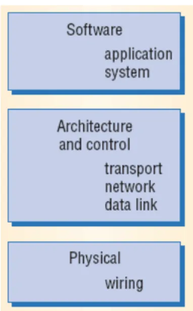
(6) Contents 摘要 ...................................................................................................................................... i Abstract..................................................................................................................................ii Acknowledgment..................................................................................................................iii Contents ................................................................................................................................ iv List of Figures....................................................................................................................... vi List of Tables ......................................................................................................................viii Chapter 1 Introduction........................................................................................................... 1 1.1. The challenges of on-chip communication........................................................ 1. 1.2. The concept of Network-on-Chip...................................................................... 2. 1.3. The focus of our work ....................................................................................... 4. 1.4. Thesis organization............................................................................................ 4. Chapter 2 Preliminary............................................................................................................ 5 2.1. Related works .................................................................................................... 5. 2.2. Our design flow ................................................................................................. 8. 2.3. Our NoC platform.............................................................................................. 9 2.3.1. Task graph............................................................................................ 11. 2.3.2. Performance evaluation ....................................................................... 13. Chapter 3 Task Scheduling .................................................................................................. 14 3.1. Assumption...................................................................................................... 14. iv.

(7) 3.2. Problem formulation........................................................................................ 17. 3.3. Genetic algorithms........................................................................................... 18. 3.4. GA-based task scheduling flow....................................................................... 20. 3.5. Initial population ............................................................................................. 21. 3.6. Evolution ......................................................................................................... 23. 3.7. 3.6.1. Selection .............................................................................................. 24. 3.6.2. Mating.................................................................................................. 24. 3.6.3. Mutation .............................................................................................. 30. 3.6.4. Simulation............................................................................................ 31. 3.6.5. Insertion............................................................................................... 35. Termination...................................................................................................... 36. Chapter 4 Experimental Results .......................................................................................... 37 4.1. Experimental flow ........................................................................................... 37. 4.2. Analysis of performance of GAs ..................................................................... 39. Chapter 5 Conclusions and Future Work............................................................................. 43 5.1. Conclusions ..................................................................................................... 43. 5.2. Future works .................................................................................................... 44. Reference ............................................................................................................................. 45 Vita....................................................................................................................................... 48. v.

(8) List of Figures Figure 1 : An NoC with 16 resources [9]............................................................................... 3 Figure 2 : Layerd-micronetwork design methodology .......................................................... 6 Figure 3 : Design flow ........................................................................................................... 9 Figure 4 : NoC platform ........................................................................................................ 9 Figure 5 : Processing element model................................................................................... 11 Figure 6 : Task graph of H.263 decoder[15]........................................................................ 12 Figure 7 : Processing element database............................................................................... 13 Figure 8 : Task graph example............................................................................................. 15 Figure 9 : Task scheduling flow........................................................................................... 20 Figure 10 : Task graph example........................................................................................... 22 Figure 11 : Generate an initial solution ............................................................................... 22 Figure 12 : The evolution flow ............................................................................................ 23 Figure 13 : Roulette wheel method ..................................................................................... 24 Figure 14 : Traditional chromosome representation............................................................ 25 Figure 15 : Traditional mating schemes .............................................................................. 25 Figure 16 : Our chromosome representation ....................................................................... 26 Figure 17 : Sub-graph crossover.......................................................................................... 27 Figure 18 : Shape of sub graph............................................................................................ 28 Figure 19 : Rotate and reflect SB ......................................................................................... 28. vi.

(9) Figure 20 : Shift SB8 close to SA .......................................................................................... 29 Figure 21 : Communication overhead of SB8 ...................................................................... 29 Figure 22 : Mutation example ............................................................................................. 30 Figure 23 : Simulation flow................................................................................................. 31 Figure 24 : Buffer length assignment .................................................................................. 32 Figure 25 : Discrete event simulation example ................................................................... 34 Figure 26 : Calculate throughput ......................................................................................... 35 Figure 27 : Insertion ............................................................................................................ 36 Figure 28 : Experimental flow............................................................................................. 37 Figure 29 : TGFF output file ............................................................................................... 38 Figure 30 : Resource location.............................................................................................. 40 Figure 31 : The improvement of 4 mating schemes ............................................................ 41 Figure 32 : Saturation time of 4 mating schemes ................................................................ 42. vii.

(10) List of Tables Table 1 : The steps of discrete event-driven simulation ...................................................... 33 Table 2 : The parameters of GAs......................................................................................... 39. viii.

(11) Chapter 1 Introduction 1.1 The challenges of on-chip communication. With the advance of technology scaling, System on Chip (SoC) designers may integrate hundreds of cores (processor, DSP, FPGA, etc.) into a single chip at the end of this decade. Current SoC designs use shared-bus architecture to connect the cores. However, this may suffer many issues in the future on-chip communication. First, since the wire delays do not scale down as good as gate delays. The global wire delay will no longer within a clock period. It is estimated that in 50nm technology, at a clock frequency of 10 GHz, a global wire delay will be 6 to 10 clock cycles. Therefore, synchronization of cores will be unfeasible [1][2][3]. Secondly, the operating frequency degrades with the increasing of number of cores attached to the bus, due to the growing of capacitive loading. 1.

(12) in its wires [4][5]. Thirdly, since the cores share the same bandwidth. System performance does not scale when integrating more cores to the system, but degrade the system performance [1][3][5]. Finally, the time to market needs to be kept as low as possible, so that reusability becomes an important issue. New bus architecture may use multiple on-chip busses which require case-specific grouping of IPs and the design of transversal bridges to provide high bandwidth, and shared-bus architecture also need an arbiter to decide which master to access the bus [3][5]. But these case-specific schemes and instance-specific designs may decrease the reusability. As a result, there should be a better design methodology to overcome these issues.. 1.2 The concept of Network-on-Chip. By borrowing the experience of computer network and parallel computing, a new design methodology called Network-on-Chip (NoC) has been proposed to solve the on-chip communication problems [2]. Network-on-Chip as its name implies is to view the system as a network of cores. In many cases, on-chip network can be designed in regular structures, so that the electrical properties of global wire are optimized and well controlled. It's helpful to enable the use of aggressive signaling circuits to reduce power dissipation [4][7]. As well, the cores communicate with each other through the network. Obviously, the NoC not only achieves the concept of Global Asynchronous Locally Synchronous (GALS) paradigm easily but also alleviate the wire delay problem and other deep sub-micro (DSM) problems. The NoC concept enables designers to design/reuse each core in one synchronous clock domain, and make the communication between cores to use message passing method through the network. Therefore, components communicate with. 2.

(13) each other asynchronously [2][5].. NoC provide better performance scalability than share-bus architecture. First, through a Peer-two-Peer communication, it can provide high bandwidth and reduce power consumption effectively. Second, by managing the network channel properly, multiple communications originated by multiple cores can be handled at the same time.. Many proposed network platforms use the regular fashion. For example, as shown in Figure 1 is a network platform with a 2D-mesh topology. Each switch is connected to its neighboring switches and a processing element.. Figure 1 : An NoC with 16 resources [9]. In such a design fashion, designers can design and verify the processing elements independently which is helpful to facilitate building a system. Moreover, designer can further build the network platform in advance and integrate with many applications [9].. 3.

(14) Therefore, we can easily amortize the development cost of network platform across many applications, and reduce time to market pressure by reusing the NoC platform.. 1.3 The focus of our work. An application can be modeled as a large number of communicating tasks. Different tasks may have different characteristics such as control or datapath. The situation implies a heterogeneous implementation including different kind of resources for different tasks tend to achieve the effective solution. Given a network platform with heterogeneous computing resources, the task scheduling problem is to decide each task being implemented with what kind of resource and which resource such that system performance is tend to be optimized. On the other hand, due to the lack of on-chip memory, we propose a task scheduling algorithm to solve this problem which optimize the system performance under memory constraints.. 1.4 Thesis organization. The rest in this thesis is organized as follows. Chapter 2 introduces related work and our design flow. Chapter 3 presents the task scheduling method using genetic algorithms. The experimental result are given and discussed in Chapter 4. Finally, the conclusions and future work are described in Chapter 5.. 4.

(15) Chapter 2 Preliminary 2.1 Related works. There are many researches in the NoC domain. By borrowing the models, techniques and tools from network and applying them to SoC design, the authors of [2] proposes a layerd-micronetwork design methodology to address future SoC designs as shown in Figure 2. In this vertical design flow, every layer is specialized and optimized for target application domain. In [7], on-chip interconnection network is used to substitute for ad-hoc global wiring structure. The structured network wiring gives well-controlled electrical parameters that eliminate timing iterations and enable the use of high-performance circuits to reduce latency and increase bandwidth.. 5.

(16) Figure 2 : Layerd-micronetwork design methodology. Recently, several NoC platforms and architectures have been proposed in [9][5][10][3]. [9] proposes a packet switched NoC platform, which includes both architecture and design methodology. The architecture is an m × n mesh of switches where the computing resources like processor core, memory, FPGA, a custom hardware or any other Intellectual Property (IP) block are connected to it. This work includes the decision of NoC architecture and the process of mapping the application onto the architecture. The Scalable Programmable Integrated Network (SPIN) is a regular, fat-tree-based network architecture [5], which uses a wormhole routing to reduce the storage requirement of network switch, and the latency of messages. A circuit switched two-dimensional mesh network called SoCBUS is proposed in [10]. [10] introduces the concept of packet connected circuit (PCC), where a packet is switched through the network locking the circuit as it goes. PCC is similar to circuit switching which has the advantages of bandwidth guarantee and deadlock-free.. 6.

(17) Some of the synthesis techniques are proposed in [3][11][12][13]. [3] presents the Xpipes which consists of a library of soft macros (switches, network interfaces and links) so that domain-specific heterogeneous architectures can be instantiated and synthesized. Xpipes provides a tool called XpipeCompiler, which can automatically instantiates a customized NoC from the library form soft network components. Precisely, the designer uses the library from Xpipes to describe the network architecture. The information on the network architecture is then specified in an input file for the XpipeComplier. The tool generates a SystemC hierarchical description of whole system. Then the description can be compiled and simulated at the cycle-accurate and signal-accurate level. [11] presents an algorithm which automatically maps the IP/cores onto a generic regular NoC architecture. This work develops an algorithm to solve the mapping problem based on branch and bound technique to minimize communication energy consumption under performance constraints. [12] presents a NMAP algorithm that maps the cores onto NOC architecture under bandwidth constraints. The NMAP can be applied on both single-path routing and split-traffic routing. In [13], the author uses a simple packet switching communication model to estimate the communication time and propose a two-step genetic algorithm to map a parameterized task graph onto the 2D-mesh NoC architecture, which minimizes the overall execution time of the task graph.. 7.

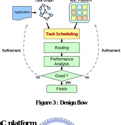
(18) 2.2 Our design flow. Figure 3 depicts our design flow. Our methodology has two input information. First, an application can be partitioned into communicating tasks. And the characteristics of tasks and their dependency is model as a task graph. Second, the NoC platform contains network architecture and heterogeneous computing resources (the task graph and NoC platform will be later explicitly explained in 2.2.1 and 2.2.2). The task scheduling process decides which task should map onto which resource. The process not only tries to reduce the communication time by mapping the interacting tasks into the same resource (make it an intra-resource communication) under memory constraints but also tries to map tasks onto the most appropriate resources to improve the computation time of each task. Next, the routing process [14] assigns a dedicated connect path for each communication between tasks. After the routing process, we can conduct a system performance analysis. If the results do not meet our requirement, we will iteratively refine our application or NoC platform and perform task scheduling and routing until the results satisfy our requirement.. 8.

(19) Task Graph. NoC Platform. Application. Task Scheduling. Routing. Refinement. Refinement. Performance Analysis no. Good ?. no. yes. Finish. Figure 3 : Design flow. 2.3 Our NoC platform. Our NoC platform is shown in Figure 4. It contains a network architecture constructed by switches, and each switch connects to a corresponding processing element. switch. switch. switch. PE. switch. PE. switch. switch. PE. switch. PE. PE. switch. PE. switch. PE. PE. Figure 4 : NoC platform. 9. PE.

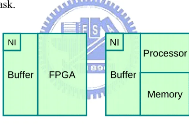
(20) The processing elements communicate to each other by passing messages through the switches of the network. Our network and switch have the following five features: (1) circuit switching, (2) dedicated connection path, (3) virtual channel flow control, (4) weighted round-robin scheduling, and (5) pipeline bus. Feature (1) and (2) provide the bandwidth guarantee and small memory usage of network switches. Feature (3) and (4) prevent deadlock and improve the utilization of network. Finally, feature (5) improves the performance of network. The details of the switch and the network architecture are explicitly described in [14].. Our NoC platform contains two types of processing elements: processor and FPGA. This makes our NoC platform a fully programmable platform. The FPGA is a dedicated hardware that can be reconfigured at run time. With a fully programmable platform, we can reduce the development cost by reusing our platform for many different applications (different. applications. with. different. configurations). without. any. architectural. modification.. The processor is a highly flexible processing element. It is good at executing tasks with the characteristics of controls. But in most cases, processors cannot provide better performance than a dedicated hardware in executing tasks with the characteristics of datapath. On the contrary, dedicated hardwares cannot be as flexible as processors. Therefore, our platform contains another type of processing element FPGA to overcome. 10.

(21) this issue. A FPGA works like a dedicated hardware but it has the advantage of being reconfigured at run time. Consequently, our platform is capable of executing various tasks efficiently.. Figure 5 shows the architectural model of our processing element. Each processing element contains a network interface to communicate with the local switch. The buffer is a temporary memory which stores the input data from other processing elements and output data to other processing elements. As mentioned before, our platform consists of two different types of processing elements. The FPGA contains a FPGA core. The processor contains a processor core and local memory which stores the program and intermediate data when executing a task.. NI. NI. Processor Buffer. Buffer. FPGA. Memory. Figure 5 : Processing element model. 2.3.1 Task graph. Applications are able to be partitioned into many communication tasks due to the parallelism. Figure 6 shows a task graph of a H.263 decoder [15]. A vertex represents a task and its functionality is shown in the vertex, too. For example, task C is IDCT which performs an inverse discrete cosine transformation of a frame produced by task B. The edge represents a data transmission and the communication amount. For example, after. 11.

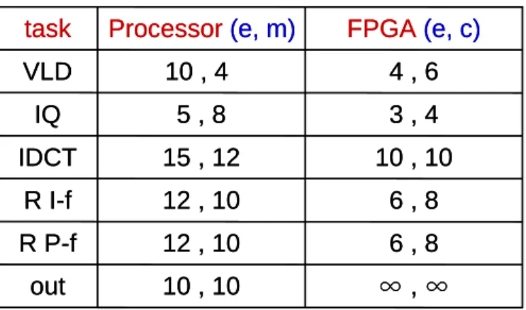
(22) task B being completed, it transmits c2 unit data to task C. An edge also indicates the data dependency. A task cannot be executed until it receives the data from its predecessor. For example, task G cannot be executed until it receives c5 unit data from task D and c6 unit data from task E. A. VLD c1 B. IQ c2 C. c3. IDCT. c4. D. E. R I-f. R P-f. c5. G. c6. out. Figure 6 : Task graph of H.263 decoder[15]. In addition to the task graph, there is a processing element database to specify the details of tasks when executing on the specific processing elements. As shown in Figure 7, a processing element database first describe the executing time of the task and the memory usage (program and intermediate data) when executing on a processor. If the task is executing on a FPGA, it shows the execution time and the capacity usage (logics) of the task. And ∞ represent that it cannot be executed on that processing element.. 12.

(23) task. Processor (e, m). FPGA (e, c). VLD. 10 , 4. 4,6. IQ. 5,8. 3,4. IDCT. 15 , 12. 10 , 10. R I-f. 12 , 10. 6,8. R P-f. 12 , 10. 6,8. out. 10 , 10. ∞,∞. e : executing time m : memory usage c : capacity usage. Figure 7 : Processing element database. 2.3.2 Performance evaluation. Since the application is not being executed only once but consecutively, we take throughput as the system performance metric, instead of the overall execution time of the application. Take the video compressing as an example. We may compress the entire movie to a more compact form, e.g. Mpeg4. A movie may contain thousands of frames. Therefore, when we are evaluating the system performance of the ability of video compressing, we may take frame per second as the rating of system performance but not second per frame. As a result, we take throughput as the metric of the system performance. More precisely, our system performance evaluation is to calculate how many times the application (task graph) can be executed in a fixed time period.. 13.

(24) Chapter 3 Task Scheduling 3.1 Assumption. Before we formulate our problem, it is necessary to define the constraints and make some assumptions.. A task can be implemented by software (program) or hardware (logics). Since the local memory of processor and total capacity of FPGA is limited, a processor cannot store infinite tasks and an FPGA cannot implement infinite tasks. Therefore, there are two constraints should be considered. The first, memory constraint of processor means that the size of the programs and intermediate data of the tasks which are stored in a processor cannot exceed the memory size of processor. The second, capacity constraint of FPGA is similar to the memory constraint. The total logics of the tasks which are implemented in a. 14.

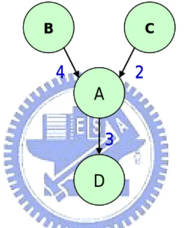
(25) FPGA cannot exceed maximum capacity of FPGA.. There should be some buffer for executing a task. For example, as shown in Figure 8, task A will be executed until it receives 4 units data from task B and 2 units data from task C. Task A needs 6 unit buffer for storing these input data temporarily. Thus the minimum requirement of input buffer in task A is 6 units. Similarly, when task A is executing, the generated output data need to be stored in output buffer. So the minimum requirement of output buffer here is 3 units. Finally, the minimum buffer requirement is 9 (6 + 3) units.. B. C. 4. 2 A 3 D. Figure 8 : Task graph example. However, it is not efficient if our buffer is only the sum of input data and output data for two reasons. First, if task A is executing, there are 4 units data from task B and 2 units data from task C in input buffer, and output buffer should prepare 3 units for task A, which means that the buffer is full. Consequently, neither task B nor task C can transmit data to task A until task A finish executing. This prevents task A from being executed continuously. Second, if task A is ready to execute, and the output buffer is full (task D does not receive data or finish receiving data from task A), task A may idle until the output buffer is clear (task D has received data from task A). As the result, the system performance may be. 15.

(26) degraded if the buffer size is only the minimum buffer requirement. Obviously, if we set our minimum buffer requirement equals to 18 units (twice of the minimum buffer requirement). The buffer works like pingpong buffer. Then, the task can receive data or transmit data no matter when the task is executing or not. It greatly improves the system performance. Hence, the reasonable buffer requirement is set to twice of the sum of input data and output data.. As mentioned before, the sum of the reasonable buffer requirement of the tasks, which are implemented with the same PE, cannot exceed the maximum capacity of buffer of PE.. If more than two tasks that are implemented on the same FPGA, it is unnecessary to decide execution order of these tasks. Since the tasks are implemented in different parts of FPGA, none of them share the same component of FPGA.. If more than two tasks that are implemented on the same processor, we make the decisions of the execution order of these tasks dynamically. Due to the dynamic behavior of communication in on-chip network, it is not suitable to decide the execution order of the tasks in design time. In addition, the application is represented as a task graph (dataflow graph) that a task is never being executed until its input data arrive.. According to these two reasons, it is suitable to use a dynamic First In First Serve (FIFS) strategy to decide the execution order of tasks. It is not only flexible to overcome the uncertainty of network, but also considering about the data availability of tasks to raise the utilization of processor [15].. 16.

(27) A FIFS strategy is implemented as a queue. If all the input data are available and output buffer size is enough, we push this task into the queue. The processor executes the tasks sequentially in order. The FIFS strategy can be further improved by either considering the data dependency or replacing it by other algorithms.. 3.2 Problem formulation. The task scheduling problem can be formulated as : Given : (1) A task graph G(V, E) and the corresponding processing element database. (2) An NoC platform which has the following characteristics: (a) mesh size, (b) local memory size of processor, (c) total capacity size of FPGA, (d) buffer size of processing element, (e) communication bandwidth of each channel, with : (1) memory and capacity constraints, and (2) buffer constraint. Determine : The allocation of each task such that system throughput is maximized.. 17.

(28) 3.3 Genetic algorithms. Basically, task scheduling is simply to allocate a set of tasks to resources such that the performance is optimal. However, it is known as NP-complete. Thus, task scheduling problem is often handled by heuristic algorithms [8][11][13][14][17].. Nevertheless, there are several important facets that influence the system performance. First, since the NoC platform contains heterogeneous computing resources, for example, a task may be suited to be executed on processor rather than on FPGA. Therefore, the execution time of a task depends on what resource that it uses. Second, the communication time between tasks highly depends on the communication distance of the resources. The communication time can be greatly improved by mapping the communicating tasks onto the same resources. However, this may violate the constraints as mentioned before. Moreover, suitability of tasks and resources are not considered. As the result, the task scheduling problem involves the trade-off among the execution time, communication time and constraints.. Typically, genetic algorithms (GAs) provide good performance at finding near-optimal solutions in a large search space. Also, unlike many traditional optimization techniques, genetic algorithms do not require the knowledge of the search-space, but need only a measure of the solution [13][18][19]. Consequently, genetic algorithms are quite suitable for the task scheduling problem.. Genetic algorithms are search algorithms based on the mechanics of natural selection. 18.

(29) and natural genetics. GAs are differ from other traditional optimization methods in four fundamental ways [18] : (1) GAs work with a coding of the parameter set, not the parameter themselves. (2) GAs search from a population of points, not a single point. (3) GAs use payoff (objective function) information, not derivatives or other auxiliary knowledge. (4) GAs use probabilistic transition rules, not deterministic rules.. The first step to employ GAs is to encode the possible solutions of the optimization problem as a set of chromosomes (the encoding scheme may differ form problem to problem, however the simplest way is to encode it into a string). Each chromosome represents a solution to the problem. And a set of solutions is referred to as a population. The next step is to generate an initial population. The chromosomes in the initial population are often generated randomly or heuristically. The initial population is also called the first generation of the evolution. Then, it is necessary to evaluate the fitness of the chromosomes, where the fitness value represents how good (fit) the chromosome is to the problem (environment).. Next, the GAs perform evolution process to optimize the population generation by generation using genetic operators: selection, mating, and mutation. During the evolution process, the GAs select chromosomes from current generation according to their fitness value, where the higher fitness the chromosome has, the higher probability it will be selected. By performing mating and mutation to the selected chromosomes, the next generation is generated by means of exploring the search-space. At last, the chromosomes. 19.

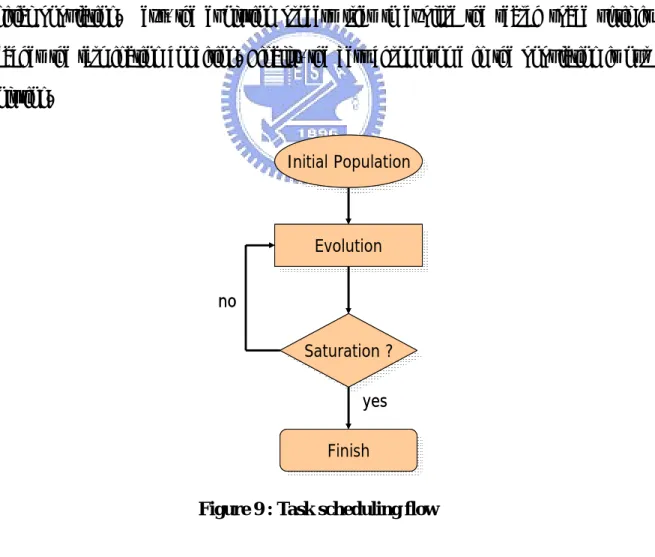
(30) in the next generation are evaluated to obtain its fitness value, and then add the next generation to the current generation. Some bad chromosomes in the population may be discarded to keep a fixed-size population.. Finally, the GAs continue evolution process until the termination condition has bean met. When the GAs terminates, the best chromosome is the final result to the problem.. 3.4 GA-based task scheduling flow. The GA-based task scheduling flow is illustrated in Figure 9. First, we generate an initial population. Next, the evolution process tries to explore the search space until it reaches the termination condition. Finally, the best chromosome in the population is our solution. Initial InitialPopulation Population. Evolution Evolution no Saturation Saturation?? yes Finish Finish. Figure 9 : Task scheduling flow. 20.

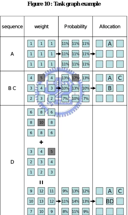
(31) 3.5 Initial population. For initial population, each chromosome is generated using a meta-random scheme which is divided into two steps: (1) The tasks in the task graph are sorted in topological order. (2) The tasks are mapped onto the NoC platform sequentially in this order. During step 2, we must consider 3 conditions: (a) If the task has no precedence, the task is mapped randomly. (b) If the task has only one precedence, the task is mapped according to the allocation of its precedence. (c) If the task has two or more than two precedence, the task is mapped according to not only the allocation of its precedence but also the communication amount between the task and its precedence.. Take the task graph in Figure 10 as an example. First, we perform topological sort on the task graph, and the topological order is given by A, B, C, D. Next, task A is randomly mapped to the NoC platform. Then, task B and task C are mapped according to the allocation of task A. As shown as Figure 11, task B and task C have higher probability to be mapped onto the allocations that close to task A. Finally, task D is mapped according to the allocations of task B and task C. Obviously, edge B→D and edge C→D has different communication amount. Therefore, the probability should be higher for the allocations that near to task B than those near to task C. Figure 11 shows how to calculate the probability of each allocation that task D are mapped.. 21.

(32) A 2. 3. B. C. 2. 1 D. Figure 10 : Task graph example. sequence. A. BC. D. weight. Probability. Allocation. A. 1. 1. 1. 11% 11% 11%. 1. 1. 1. 11% 11% 11%. 1. 1. 1. 11% 11% 11%. 4. 5. 4. 13% 17% 13%. A. 3. 4. 3. 10% 13% 10%. B. 2. 3. 2. 7%. 10%. 6. 8. 6. 8. 10. 8. 6. 8. 6. 3. 4. 5. 2. 3. 4. 1. 2. 3. 9. 12. 11. 9%. 13% 12%. 10. 13. 12. 11% 14% 13%. 7. 10. 9. 8%. 11%. 7%. A BD. 9%. Figure 11 : Generate an initial solution. 22. C. C.

(33) During the process of generating a chromosome, the constraints are also needed to be considered. The tasks cannot be assigned to the allocations in which the constraints may be violated. The initial population is generated with a fixed number of chromosomes which is generated by the meta-random scheme. Then, the fitness value of each chromosome is evaluated.. There are two reasons why we use a meta-random scheme to generate a chromosome. First, a pure random scheme may cause a very bad performance. Second, the diversity of the chromosomes in the initial population should be kept as high as possible so that the GAs have higher probability to explore larger search-space. Due to these two reasons, we use a meta-random scheme to generate the chromosomes which not only consider the performance issue but also the diversity issue.. 3.6 Evolution. GAs try to explore the search space using the three genetic operators: selection, mating, and mutation. The evolution flow is illustrated in Figure 12. Initial InitialPopulation Population. Selection Selection. Evolution Evolution. Mating Mating && Mutation Mutation. Saturation Saturation??. Simulation Simulation. no. yes. Insertion Insertion. Finish Finish. Figure 12 : The evolution flow. 23.

(34) 3.6.1 Selection. Due to the principle of eugenics, an individual (chromosome) which has higher fitness value has higher probability to produce next generation. Therefore, we select pairs of parents from the population using roulette wheel method [18]. Each chromosome in the population has roulette wheel slot sized in proportion to its fitness value. Then the chromosome is selected by spinning the roulette wheel. Take Figure 13 as an example, chromosome A has the largest fitness value, so it occupies the largest size in the roulette wheel. By spinning roulette wheel many times, the selected chromosomes are going to mate in the next step.. chromosome. fitness. A B C D E. 5 4 2 3 1. E. spin A. D C B. Figure 13 : Roulette wheel method. 3.6.2 Mating. GAs use mating to explore the search space and try to find the local optimal. In the nature, the children inherit the features from parents. For example, if parents have big eyes, their children usually have big eyes, too. So as in GAs, the generated chromosomes inherit the features from their parents.. 24.

(35) First of all, it is needed to explain how the traditional mating scheme works. But, before we talk about the traditional mating scheme, it is necessary to introduce the traditional representation of chromosomes. Each chromosome is represented as a string, and each word in the string represents the allocation of the corresponding task. As shown in Figure 14, the chromosome is represented as a string {(0,0), (1,1), (2,1), (3,1), (1,1)}, which indicates that task A is in (0,0), task B is in (1,1), and so on. col A row. BE. C D. {(0,0), (1,1), (2,1), (3,1), (1,1)} (row, col). Figure 14 : Traditional chromosome representation. The traditional mating schemes consist of single-point crossover, two-point crossover, etc. As illustrate in Figure 15, single-point crossover first randomly selects a cross point of two parents, and then exchange the sub-string between the cross point and the end of the string. As the name implies, two-point crossover use two randomly selected cross points to choose the sub-string to be exchanged. However, both of these two mating schemes do not consider the dependency of tasks. Single-point crossover. Two-point crossover. Parents. Parents. Children. Children cross point. cross point. Figure 15 : Traditional mating schemes. 25.

(36) Unlike the traditional mating schemes, we propose two different mating schemes which consider the dependency of tasks to obtain better performance in communication. Different from the traditional representations, the representation of our chromosome is a graph, where each word in the vertex indicates the allocations of corresponding tasks. As illustrated in Figure 16, the top vertex of the chromosome indicates that task A is in (0,0), the top-right vertex indicates that task B is in (1,1), and so on. Hence, our representation is capable of representing the dependency between tasks where the string representation cannot provide these important information. A. 0,0. col A. C B. row. 2,1 C. D E Task graph. 1,1. BE. 3,1. D Solution. 1,1 Chromosome. Figure 16 : Our chromosome representation. The first mating scheme we proposed is sub-graph crossover which exchanges a sub-graph in a well-coded representation. Figure 17 illustrates the exchanging process of sub-graph crossover. At first, we randomly select a number x between 1~n-1 (where n is the total task number). Second, we randomly choose a task at the task graph and then perform breadth first search (BFS) starting from task until the number of visiting tasks reaches x. At last, the sub-graph is found, and we can exchange the sub-graph to produce the next generation.. 26.

(37) Parents. A. exchange. 0,0. 1,2. Children. B 2,3. 1,1. 1,4. A’. 0,2. 1,2. 3,1. 4,0 2,2. 2,1. 1,1 1,2. 1,3. 3,0 2,1. 2,1. 3,0. 2,0. 1,1. 1,4 3,0. 2,1. 0,2. 2,3. 3,1. 4,0. 1,3 2,0. B’. 0,0. 1,1 3,0. 2,0 2,1. 2,2 2,1. 1,2. 1,3 1,3. 3,0. 2,0. 2,1 2,1. 3,0. Figure 17 : Sub-graph crossover. Although sub-graph crossover considers the dependency of tasks, it is still not good enough. It can be further improved by taking the suitability between the parents and the exchanged sub-graph into account. The higher fitness the chromosome has, the higher probability the chromosome will be selected to be parent. In other words, the selected parents usually provide good performance. It is not wise to change the parents in a big way, because this may destroy the original structure of parents and then get a bad chromosome. Hence, shape crossover is proposed to raise the suitability between the parents and the exchanged sub-graph. As shown in Figure 18, the allocations of tasks in the sub-graph construct a shape. Obviously, if we exchange SA and SB directly in the absolute position, it will destroy the original structure. Since the communication between original A and SA may be good. But after exchanging, original A and SB may be too far to communicate to each other. Therefore, the clever way is to exchange SB and SA in the relative position, and then the structure is not destroyed but makes a little change.. 27.

(38) A. B. 0,0. 1,2. 2,3. 1,1. 1,4. A. 0,2. B. 3,1. 4,0 2,2. 2,1. 1,1 1,2. 1,3. SA. 3,0 2,1. 3,0. 2,0. SB. 1,3. SA. 2,1 2,1. 2,0. SB. 3,0. Figure 18 : Shape of sub graph. The details of shape crossover are described as following steps:. Assume dad A and mom B produce son C. (1) Randomly choose a sub-graph, and then find the allocations of the corresponding tasks, which construct a shape. Take Figure 18 as an example, the allocations of the corresponding tasks are SA and SB, respectively. (2) Rotate and reflect SB in 8 conditions (rotate 0°, 90°, 180°, 270° and reflect the above) which is illustrated in Figure 19. And then shift these shapes to an appropriate position which makes the gravity center of each shape as close as to that of SA. Figure 20 shows the process of shifting SB8 to SA. rotate 0° SB1. rotate 90° SB2. SB3. reflect. reflect SB5. rotate 180°. SB6. rotate 270° SB4. reflect SB7. reflect SB8. Figure 19 : Rotate and reflect SB. 28.

(39) shift. gravity center of SA. gravity center of SB8. Figure 20 : Shift SB8 close to SA. (3) After step (2), we get 8 solutions. It is necessary to estimate which solution is the best among these 8 solutions. The way we estimate these solutions is to calculate the communication overhead that they cause. The communication overhead is defined as Σci*di where ci is input or output communication amount of the sub-graph and di is the Manhattan distance of that communication. For example, the communication overhead of SB8 = 5*1+4*4+2*2+3*1+2*3+1*4 = 38 which is shown in Figure 21. The first term 5*1 is the top left vertex of the sub-graph where 5 is the communication amount, 1 is the Manhattan distance between (1,2) and (1,1), and so on. 0,0. 4. 1,2. 2,2. 5 1,1. 2 1,2. 2,1. 1,1 1,2 3. 1,3. 1. 2. 1,3. 2,0. Figure 21 : Communication overhead of SB8. 29.

(40) After calculating the communication overhead of these 8 solutions, the final result is the solution with minimum communication overhead that causes by SB.. During the step (2), some of the tasks may violate the constraints and lead to an infeasible solution. Therefore, we must repair the tasks which violate the constraints. The repair method is similar to the second step in generating the chromosome of the initial population. The different is that we just map the tasks which violate the constraints but not all tasks in the task graph.. 3.6.3 Mutation. The goal of mutation is to prevent GAs from finding just local optimal. By randomly change the feature of the chromosome, the chromosome may have the opportunity to reach or get close to the global optimal. Our mutation scheme first selects a task at random. Next, the selected task has a probability to move to a random allocation. Also, the new allocation must satisfy the constraints. Here is an example in Figure 22. A. A. D C E. D C B. B E. 1. Randomly select a task : task E. 2. Randomly move to new allocation. Figure 22 : Mutation example. 30.

(41) 3.6.4 Simulation. After mating and mutation, it is necessary to evaluate the fitness value of each new generated chromosome. We use high-level simulation to obtain the throughput of every new generated chromosome. Figure 23 demonstrates our simulation flow.. Initial InitialPopulation Population. no. Selection Selection. Evolution Evolution. Mating Mating && Mutation Mutation. Saturation Saturation??. Simulation Simulation. yes. Buffer Bufferlength length assignment assignment Discrete Discrete event-driven event-driven simulation simulation Calculate Calculatethe the throughput throughput. Insertion Insertion. Finish Finish. Figure 23 : Simulation flow. At first, the buffer length assignment of each task is conducted. We assign input and output buffer to every task equally and make sure that each task has one input and output buffer shown in Figure 24.. 31.

(42) NI. Buffer buffer. T1. T3. T3. T1. Figure 24 : Buffer length assignment. Second, since there are many dynamic behaviors when executing the application (task graph) consecutively using our platform, and the time to find out the throughput of the chromosome must be short. It is not feasible to use a simple scheduling scheme or a simulation in the cycle-accurate level to obtain the throughput of each chromosome. Therefore, by considering both the dynamic behaviors and time issue, we use a discrete event-driven simulation in signal-accurate level to evaluate each chromosome. In this environment, each communication time must be estimated in a fixed value. For simplicity, XY routing is used to route the communication paths. By assuming that contention always happens, the communication time is estimated under pipeline manner [14].. There are two kinds of event in this discrete event-driven simulation: computation event and communication event. The computation event of a task represents that the task finish executing, and is ready to transmit data to its successors. In FPGA, when all input data arrive and the output buffer size is large enough, the computation event is inserted into the time queue with the time equals to the current time plus computation time. In processor,. 32.

(43) the event will not be directly inserted to the time queue, but arranged by the scheduler (FIFS) of processor that we mentioned before. The communication event between tasks represents that the successor receives data from predecessor. When the input buffer of the successor is large enough, the communication event is inserted to the time queue with the time equals to the current time plus communication time. Figure 25 shows an example, where the number in the vertex is the computation time of the task, and the number on the edge is the communication time of the data transmission. Table 1 explicitly describes the steps of the simulation.. step 1 :. Current time = 3, execute computation event A.. step 2 :. Current time = 3, after executing computation event A, the data is transmitted to task C, and then it arrives at time = 3+5=8, therefore insert a communication event A→C with time = 8.. step 3 :. Current time = 4, execute computation event B.. step 4 :. Current time = 4, after executing computation event B, the data is transmitted to task C, and then it arrives at time = 4+3=7, therefore insert a communication event B→C with time = 7.. step 5 :. Current time = 7, the data is transmitted from task B to task C.. step 6 :. Current time = 8, the data is transmitted from task A to task C.. step 7 :. Current time = 8, since all input data of task C arrive, insert a computation event of task C with time = 8+2=10.. step 8 :. Current time = 10, execute computation event C. Table 1 : The steps of discrete event-driven simulation. 33.

(44) 1. A 3. B 4. 3 C. A B. 5. B->C A->C. 2. C. 3 3. D. 3. A 4. 3 C. A B. 5 2. C. 3 3. D. 5. A 4. C. A B. 5. 3. B->C A->C. 2. C. 3 3. D. 7. A 4. 5. 3 C. B->C A->C. 2. 3 3. D. A B. C. 3. C. A B. 5. 3 2. A->C C. 3 3. D. 4. A 4. 3 C. A B. 5. B->C A->C. 2. C. 3 3. D. 6. A 4. C. A B. 5. 3. B->C A->C. 2. C. 3 3. D. 8. A 4. 5. 3 C. 3 3. D. Figure 25 : Discrete event simulation example. 34. A B B->C A->C. 2. 0 1 2 3 4 5 6 7 8 9 10 11 12 13 14 15. time queue. 3. B. 0 1 2 3 4 5 6 7 8 9 10 11 12 13 14 15. 0 1 2 3 4 5 6 7 8 9 10 11 12 13 14 15. time queue. 3. B. 0 1 2 3 4 5 6 7 8 9 10 11 12 13 14 15. 0 1 2 3 4 5 6 7 8 9 10 11 12 13 14 15. time queue. 3. B. 0 1 2 3 4 5 6 7 8 9 10 11 12 13 14 15. time queue. 3. B. time queue. 4. time queue. 3. B. A B. 0 1 2 3 4 5 6 7 8 9 10 11 12 13 14 15. time queue. 3. B. 2. time queue. C. 0 1 2 3 4 5 6 7 8 9 10 11 12 13 14 15.

(45) By continuously input the data to the NoC platform, the output data are sequentially generated at different times, which are recorded to the profile. After simulation, we are able to calculate the throughput of the chromosome from the profile. The data generation rate is taken as system throughput when the system is stable. As shown in Figure 26, data generation rate equals 0.8 (4/5).. input data 0. NoC Platform 5. output data. 10. 15. time stable. : output data. Figure 26 : Calculate throughput. 3.6.5 Insertion. The last step of evolution is insertion. After calculate the fitness value of every new chromosome, we insert these chromosomes into current population. Due to the population size being fixed, we must remove some chromosomes. According to selection of natures, the redundant chromosomes with low fitness value are discarded. Here is an example in Figure 27. After we insert new chromosomes to current population, we sort the population in decreasing order by fitness value. And then the bad chromosomes are discarded to keep a fixed-size population.. 35.

(46) current sort. remove. new Figure 27 : Insertion. 3.7 Termination. GAs terminate until the fitness value of the best chromosome is saturated during the evolution process or the generation number reaches a pre-defined number.. 36.

(47) Chapter 4 Experimental Results 4.1 Experimental flow. Figure 28 demonstrates our experimental flow. At first, we exploit Task Graphs for Free (TGFF) [20] , which is a user-controllable, general-purpose, pseudorandom task graph generator, to generate random cases. And then, the generated task graphs are scheduled by our task scheduling tool. Finally, we can analyze the experimental results.. TGFF. Task Scheduling. Task Graph. Figure 28 : Experimental flow. 37. Analysis.

(48) We use TGFF to generate many task graphs. Each task graph contains a netlist and tables for related information. For example, Figure 29 (a) is a netlist, where “TASK” represents a task and the following are the task name and computation information which is specified in Figure 29 (c) (processing element database). As well, “ARC” represents a data transmission from the former to the later, and the corresponding communication amount is given in Figure 29 (d). In the computation table, “uP” and “fpga” represent the computation time in processor and FPGA, respectively. “memory” and “capacity” are the memory and capacity usage of processor and FPGA. The TGFF output file and its corresponding task graph is shown in Figure 29 (b).. @TASK_GRAPH 0 { PERIOD 1659 TASK t0_0 TASK t0_1 TASK t0_2 TASK t0_3. TYPE 2 TYPE 73 TYPE 14 TYPE 51. ARC a0_0 ARC a0_1 ARC a0_2 ARC a0_3. FROM t0_0 FROM t0_0 FROM t0_1 FROM t0_2. 35. t0_0 2. t0_1 14 TO TO TO TO. t0_1 TYPE 35 t0_2 TYPE 11 t0_3 TYPE 30 t0_3 TYPE 47. 11 t0_2 73. 30. 47 t0_3 51. }. (a) Netlist. (b) Task graph. @computation 0 { #---------------------------------------------------------------# type uP memory fpga capacity 0 55.7067 163.892 151.128 178.518 1 64.9349 152.398 159.265 175.757 2 75.4444 160.801 166.259 193.153 3 52.5038 157.158 152.051 153.982 4 66.1995 175.019 170.291 192.132 5 56.5161 151.905 154.492 159.021. @communication 0 { #----------------------------------------# type amount 0 155.707 1 151.676 2 158.991 3 153.979 4 194.139 5 160.684. . .. . .. }. }. (c) Computation table. (d) Communication table. Figure 29 : TGFF output file. 38.

(49) 4.2 Analysis of performance of GAs. In this experiment, we compare the traditional mating schemes and our mating schemes. The parameters of GAs are shown in Table 2.. Cross rate. 40%. Mutation rate. 20%. Population. 400. Max generation. 1000. Table 2 : The parameters of GAs. Cross rate means that 40% of population is going to mate. Mutation rate means that every new generated chromosome has the probability of 20% to perform mutation. The whole population is set to 400 chromosomes. The algorithm terminates until the performance of the best chromosome is saturated or when it reach max generation.. We generate 20 random task graphs and each task graph contains 270 ~ 330 tasks. The computation time of each task is set to 150 ~ 200 time unit on FPGA and 50 ~ 67 time unit on processor. When two or more than two tasks that are mapped onto a processor, the processor needs to schedule the tasks. Therefore, we set the computation time of each task on processor 1/3 times of that on FPGA, such that total computation time of tasks on processor or FPGA is more balance. The communication amount is 150 ~ 200 data unit, and the maximum fanin/out of each task is 6. The memory and capacity usage of each task is set to 150 ~ 200.. 39.

(50) The communication time is the communication amount divided by channel bandwidth without any contention. Here, the channel bandwidth is set 1 ~ 4 (data unit / time unit), such that the ratio of computation time to communication time (no contention) is 1 ~ 4. When the ratio is low (e.g., 1), the system is computation intensive. When the ratio is high (e.g., 4), the system is communication intensive.. The resource location of our platform is shown in Figure 30. The topology is like a chessboard, and the mesh size is 7 × 7. The memory of processor and capacity of FPGA are set to 1800. The buffer size of each PE is 12000 (data unit).. Processor. FPGA. Figure 30 : Resource location. The system performance improved rate of four mating schemes with four ratio (1~4) are shown in Figure 31. Since sub-graph crossover considers the dependency of tasks, the improved rate of GAs that using sub-graph crossover outperforms those use traditional single point-crossover and two-point crossover. This implies that the mating schemes should consider the dependency of tasks. In addition, shape crossover not only inherits the features of sub-graph crossover but also consider about the suitability issues. As a result,. 40.

(51) shape crossover outperforms all other mating schemes. In Figure 32, the saturation time of shape crossover is less than others. Shape crossover provides better results and shorter computation times than other mating schemes.. Improve rate = Communication intensive. Computation intensive. (Tx - Trandom) Trandom. , Ratio = comp. time / commu. time. Ratio. random. 1 point. 2 point. sub-graph. shape. 1. 0%. 120%. 123%. 129%. 139%. 2. 0%. 124%. 135%. 140%. 150%. 3. 0%. 124%. 131%. 133%. 140%. 4. 0%. 123%. 126 %. 137%. 139% *Average of 20 cases. 160% 140% 120% 100% 80% 60% 40% 20% 0%. random. 1p. 2p. sub-g. shape. 1. 2. 3. 4. Figure 31 : The improvement of 4 mating schemes. 41.

(52) Saturation time (generation) Ratio. 1 point. 2 point. sub-graph. shape. 1. 845. 801. 786. 765. 2. 843. 845. 861. 832. 3. 866. 836. 818. 811. 4. 840. 838. 824. 711 *Average of 20 cases. 880 860 840 820 800 780 760 740 720 700. 1p 2p sub-g shape. 1. 2. 3. 4. Figure 32 : Saturation time of 4 mating schemes. 42.

(53) Chapter 5 Conclusions and Future Works 5.1 Conclusions. In this thesis, we solve the multi-constraints task scheduling problem. By mapping the task scheduling problem to GA-domain, this problem is solved in an efficient way. Since the traditional mating schemes in GAs do not consider the dependency of the task graph, we propose both sub-graph and shape crossover to overcome this issue. We also construct a high-level simulator to evaluate our solutions. This is not only fast but also accurate. The experimental results show that our mating schemes provide better performance and require less computation time than traditional ones.. 43.

(54) 5.2 Future works. It is found that buffer-size for every input/output of task has great impact on system performance. If the buffer-size is unlimited, the data transmission can always be accepted, and the utilization of communication resources will be maximized so that system performance is also improved. However, due to the lack of on-chip memory, unlimited buffer-size is impossible. An algorithm must be developed to optimize the buffer-length of each input/output instead of equally-distributed, such that the system performs well with limited buffer size.. Resource location is also important. If we do not consider the relationship between topology of resource location and application, the system may not perform well. Consequently, given a specific application and several platforms with different topologies, an algorithm must be developed to find out the most suitable platform for the application.. 44.

(55) Reference [1]. Axel Jantsch and Hannu Tenhunen, Networks on Chip, Kluwer Academic Publishers, 2003.. [2]. Luca Benini and Giovanni De Micheli, “Networks On Chips: A New SoC Paradigm,” in Computer Jan. 2002, Volume 35, Issue 1, pp. 70-78.. [3]. Davide Berozzi and Luca Benini, “Xpipes: A Network-on-Chip Architecture for Gigascale Systems-on-Chip,” in Circuit and Systems Magazine 2004, Volume 4, Issue 2, pp. 18-31.. [4]. Cesar Albenes Zeferino and Altamiro Amsdeu Susin, “SoCIN: A Parametric and Scalable Network-on-Chip,” in Proceedings of the 16th Symposium on Integrated Circuits and Systems Design, Sep. 2003, pp. 169-174.. [5]. Pierre Guerrier and Alain Greiner, “A Generic Architecture for On-Chip Packet-Switched Interconnections,” in proceedings of the conference on Design, automation and test in Europe, 2000, pp. 250-256.. [6]. Alan Allan, Don Edenfeld, William J. Joyber, Jr, Andrew B. Kahng, Mike Rodgers and Yervant Zorian, “2001 Technology Roadmap for Semiconductors,” in IEEE computer, Jan. 2002, pp.42-53.. [7]. William J. Dally and Brian Towles, “Route Packets, Not Wires: On-Chip Interconnection Networks,” in Proceedings of the Design Automation Conference, June 2001, pp. 684-689.. [8]. Jingcao Hu and Radu Marculescu, “Energy- and Performance-Aware Mapping of Regular NoC Architectures,” on IEEE transactions on Computer-Aided Design of. 45.

(56) Integrated Circuits and Systems, April 2005, Volume 24, Issue 4, pp.551-562. [9]. Shashi Kumar, Axel Jantsch, Juha-Pekka Soininen, Martti Forsell, Mikaek Millberg, Johny Öberg, Kari Tiensyrjä and Ahmed Hemani, “A Network on Chip Architecture and Design Methodology,” in Proceedings of IEEE Computer Society Annual Symposium on VLSI, April 2002, pp. 105-112.. [10] Daniel Wiklund and Dake Liu, “SoCBUS: Switched Network on Chip for Hard Real Time Embedded Systems,” in Proceedings of the Parallel and Distributed Processing Symposium, April 2003. [11] Jingcao Hu and Radu Marculescu, “Energy-Aware Mapping for Tile-based NoC Architectures Under Performance Constraints,”. in Proceedings of Asia & South. Pacific Design Automation Conference, Jan. 2003, pp. 233-239. [12] Srinivasan Murali and Giovanni De Micheli, “Bandwidth-Constrained Mapping of Cores onto NOC Architectures,” in Proceedings of the Design, Automation and Test in Europe Conference and Exhibition, Feb. 2004, volume. 2, pp. 896-901. [13] Tang. Lei and Shashi Kumar, “A Two-Step Genetic Algorithm for Mapping Task Graphs to a Network on Chip Architecture,” in Proceedings of Euromicro Symposium on Digital System Design, Sep. 2003, pp. 180-187. [14] Liang-Yu Lin, Cheng-Yeh Wang, Pao-Jui Huang, Chih-Chieh Chou and Jing-Yang Jou, “Communication-driven Task Binding for Multiprocessor with Latency Insensitive Network-on-Chip,” Asia and South Pacific Design Automation Conference, Jan. 2005. [15] R.J.H. Hoes, “Predictable Dynamic Behavior in NoC-based Multiprocessor System-on-Chip,” M.Sc. Thesis, TUE, Eindhoven, Dec. 2004. [16] Edward Ashford Lee and Soonhoi Ha, “Scheduling Strategies for Multiprocessor. 46.

(57) Real-Time DSP,” in Global Telecommunication Conference and Exhibitions, Nov. 1989, Volume 2, pp. 1279-1283. [17] Kenjiro Taura and Andrew Chien, “A Heuristic Algorithm for Mapping Communicating Tasks on Heterogeneous Resources,” in Proceedings of 9th Heterogeneous Computing Workshop, May 2000, pp. 102-115. [18] David E. Goldberg, Genetic Algorithms in Search, Optimization & Machine Learning, Addison-Wesley Publishers, 1989. [19] Baxter, M. J., Tokhi, M. O. and Fleming, P. J. “An Investigation of the Heterogeneous Mapping Problem Using Genetic Algorithms,” on CONTROL '96, UKACC International Conference, Sep. 1996, Volume 1, pp. 448-453. [20] Robert P. Dick, David L. Rhodes and Wayne Wolf, “TGFF: Task Graphs for Free,” in proceeding of the 6th International Workshop on Hardware/Software Codesign, 1998, pp. 97-101.. 47.

(58) Vita Wan-His Hsieh was born in Taoyuan, Taiwan on August 6, 1981. He received the B.S. degree in Electrical Engineering from National Central University in June 2003 and entered the Institute of Electronics, National Chiao Tung University in September 2003. His research interests include electronic design automation (EDA) and VLSI design. He received the M.S. degree from National Chiao Tung University in June 2005.. 48.

(59)