從最佳化觀點推導多評準分類規則— 以生物及醫療資訊為例

國立交通大學

資訊管理研究所

博士論文

從最佳化觀點推導多評準分類規則

—

以生物及醫療資

訊為例

Induction of Multiple Criteria Classification Rules from

Optimization Perspectives — Applied in Biology and

Medicine Informatics

研究生

:

陳明賢

指導教授

:

黎漢林 博士

從最佳化觀點推導多評準分類規則

—

以生物及醫療資

訊為例

Induction of Multiple Criteria Classification Rules from

Optimization Perspectives — Applied in Biology and

Medicine Informatics

研究生

:

陳明賢

Student: Ming-Hsien Chen

指導教授

:

黎漢林

Advisor: Han-Lin Li

國立交通大學 資訊管理研究所

博士論文

A Dissertation

Submitted to Institute of Information Management College of Management

National Chiao Tung University in Partial Fulfillment of the Requirements

of the Degree of

Doctor of Philosophy in Information Management June 2008

Hsinchu, Taiwan, Republic of China

從最佳化觀點推導多評準分類規則

—

以生物及醫療資

訊為例

學生

:

陳明賢

指導教授

:

黎漢林

摘

要

Induction of Multiple Criteria Classification Rules from

Optimization Perspectives — Applied in Biology and

Medicine Informatics

Student: Ming-Hsien Chen

Advisor: Han-Lin Li

Institute of Information Management National Chiao Tung University

Abstract

To induce critical classification rules from observed data is a major task in biological and medical research. A classification rule is considered to be useful if it is optimal and simultaneously satisfies three criteria: is highly accurate, has a high rate of support, and is highly compact. However, existing classification methods, such as rough set theory, neural networks, ID3, etc., may only induce feasible rules instead of optimal rules. In addition, the rules found by existing methods may only satisfy one of the three criteria. This study proposes a multi-criteria model to induce optimal classification rules with better rates of accuracy, support and compactness. A linear multi-objective programming model for inducing classification rules is formulated. Two practical data sets, one of HSV patients results and another of European barn swallows, are tested. The results illustrate that the proposed method can induce better rules than existing methods.

Acknowledgement

正如當年完成碩士論文時的誌謝

,

首先依然是要感謝我的父母、 陳建

仁先生及葉惠美女士的支持與鼓勵

,

並提供一個無後顧之憂的環境

,

讓我再次於離開學校多年後

,

二度拋下工作

,

繼續進修

,

全心全意投

入本研究。 因為有他們對我的愛護

,

我才有可能完成學業。

接著

,

要感謝黎漢林教授多年來的悉心指導

,

使我不論是在學業、

思維或為人處事上

,

皆有長足的進步

,

於此特別表示由衷的謝意。

同時

,

要感謝曾國雄教授、 溫于平教授、 陳茂生教授、 林妙聰教授

及李永銘教授的指正與建議

,

及林信雄教授的英文寫作指導

,

使本論

文得以更加完善。

此外

,

要感謝陳煇煌教授、 蘇宜芬老師及柯宇謙老師鼎力關照

,

介

紹兼課機會

,

使我在博士修業期間

,

不但生計不虞匱乏

,

且能娶妻生

子、 並完成學業。

再者

,

要感謝運籌管理研究室的伙伴們

,

昶瑞、 宇謙、 麗菁、 浩鈞、

芸珊、 嘉輝、 曜輝、 婉瑜等人

,

陪我一同走過這漫長的研究之路

,

無論

是生活上的扶持

,

或是學業上的切磋砥厲

,

都給我莫大的助益。

最後

,

我要將接下來的篇幅

,

留給我的妻子、 李益芬

,

因為有她的

支持、 體諒及無怨的付出

,

我才能熬過低潮

,

完成這個研究。 結婚這

幾年來

,

聚少離多

,

她不但經常孤單在家

,

還歷經患甲亢、 懷孕、 生

子、 育嬰、 再懷孕

,

然她都不畏艱苦、 一肩扛起

,

讓我全心投入學業。

今日的成果

,

全因有她成就

,

在此

,

我不但要感謝她

,

還要將這論文獻

給她。

Contents

List of Figures vii

Chapter 1 Introduction 1

1.1 Research Background . . . 1

1.2 Review of Some Existing Methods . . . 3

1.2.1 Review of Rough Set Theory . . . 3

1.2.2 Review of ID3 . . . 4

1.3 Research Objectives . . . 4

1.4 Structure of the Dissertation . . . 5

Chapter 2 Problem Formulation and Notations 6 2.1 Problem Formulation . . . 6

2.2 Presentation of Data and Rules . . . 6

2.3 Notations and Variables Summary . . . 10

Chapter 3 Proposed Classification Method 13 3.1 Propositions . . . 13

3.3 Models for Inducing Rules . . . 18

3.4 Analysis of Models . . . 24

Chapter 4 Experiments 26 4.1 The HSV Patients Data Set . . . 26

4.1.1 Rules Induced by RST and ID3 . . . 28

4.1.2 Rules Induced by the Proposed Method . . . 28

4.1.3 Comparison of Results . . . 30

4.2 The European Barn Swallow Data Set . . . 32

4.2.1 Rules Found by VPRS and ID3 . . . 32

4.2.2 Rules Induced by the Proposed Method . . . 34

4.2.3 Comparison of Results . . . 35

Chapter 5 Implementation 36 Chapter 6 Discussions and Remarks 43 6.1 Discussions . . . 43

6.2 Remarks . . . 43

References 45

Appendices 48

A The HSV Patients Data Set 48 B The European Barn Swallow Data Set 51 C The Input Data File Format for MCOCR 53 D A Sample Input Data File for MCOCR 57

List of Tables

2.1 A small data set . . . 7

2.2 Binary presentation for the data set in Table 2.1 . . . 8

2.3 Some rules for Table 2.1 . . . 9

2.4 The explanation for rules in Table 2.3 . . . 11

4.1 Norms for attributes of the HSV data set . . . 27

4.2 The best rule for each class of HSV found by ROSE2 . . . 28

4.3 Comparison of the proposed method, ROSE2 and ID3 for the HSV data set. . . 31

4.4 Norms for attributes of the European barn swallow data set . 32 4.5 Rules for swallow data set found by VPRS . . . 33

4.6 Some better rules for swallow data set found by ID3 . . . 33

4.7 Rules for swallow data set found by the proposed method . . . 34

A.1 The HSV patients data set with original values of attributes . 49 B.2 The European barn swallow data set with original values of attributes . . . 51

List of Figures

4.1 A partial ID3 decision tree for HSV data set. . . 29

4.2 The ID3 decision tree for swallow data set. (Beynon and

Buchanan, 2003) . . . 34

5.1 Step1: Click ”Select Data File” button to select an input data

file . . . 38

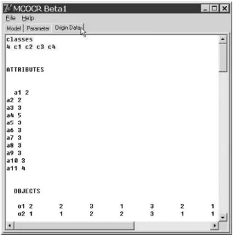
5.2 After chosen an input data file, the “Origin Data” tag appears. 38

5.3 Click ”Origin Data” tag, the contents of the input file will be

displayed on the window. . . 39

5.4 Select an objective. The ”max CR” is chosen, here. Specify

Lower Bounds. The AR is specified as 1 and the number of supporting objects is specified as 3, here. Specify the class to classify. Here is 2. Click ”Generate Program” button to

generate LINGO program. . . . 39

5.5 After ”Generate Program” button clicked, the ”Program” tag

appears. . . 40

5.6 Click ”Program” tag, the contents of the generated Lingo

pro-gram will be displayed on the window. . . 40

5.7 Step 6: Click ”Induce Rule” button to start inducing rules. . . 41

5.8 The ”Result” tag will appear while a rule generated and

gen-erated rules will be displayed on the window. . . 41

5.9 Click ”Induce Next Rule” button to induce another rule. . . . 42

Chapter 1 Introduction

1.1

Research Background

The induction of classification rules1 _{from a database has been one of the}

major issues in the biological and medical research domains. Given a data set with several objects, where each object has some attributes and belongs to a specific class, the induction of rules is to find a combination of attributes which can well describe the features of a specific class. There are three criteria for evaluating the quality of a rule.

(i) Accuracy. A good rule which fits a specific class had better not cover objects of other classes.

(ii) Support. A good rule which fits a specific class should be supported by most objects of such a class.

(iii) Compactness. A good rule should be expressed in a compact way. That means that the less the number of attributes used, the better the rule is.

Currently, there are some well-known methods for classification, especially the rough-set-based method and the decision-tree-based method.

In Hvidsten et al. (2003), rough sets were used as the theoretical founda-tion for its methodology to learn the rule-based biological process from gene expression time profiles. It reported a systematically supervised learning ap-proach to predict a biological process from the time series of gene expression 1_{Instead of using the term “classification rule”, the term “rule” is used for short in the}

data and biological knowledge. Biological knowledge is expressed using gene ontology and this knowledge is associated with discriminatory-expression-based features to form minimal decision rules. In Beynon and Buchanan (2003), which used variable precision rough sets, a variant of rough sets, to do the gender classification of the European barn swallow. Slowinski (1992), Tsumoto (1999), Li and Wang (2004), Tay and Shen (2002), Shen and Loh (2004), etc., also used the rough-set- based method to get rules.

In Geurts et al. (2005), the decision-tree-based method was used for pro-teomic mass spectra classification. They proposed a systematic approach based on decision-tree-ensemble methods, which is used to automatically de-termine proteomic biomarkers and predictive models. Aja-Fernandez et al. (2004)proposed a fuzzy ID3 decision-tree methodology by which the natu-ral language descriptions of the TW3 method for bone age assessment is

translated into an automatic classifier. And in Zhang et al. (2001), the

decision-tree-based method was used for classifying normal or tumor tissues, etc.

Both the rough set based method and the decision tree based method are heuristic algorithms, which are computationally effective in inducing rules. However, there are two shortcomings for these two methods:

(i) They may find only some feasible rules, instead of inducing optimal rules.

(ii) For most cases, they may find only rules satisfying a single criterion such a more accuracy rate or a more support rate, instead of inducing rules to satisfy multiple criteria.

1.2

Review of Some Existing Methods

There are many well-known methods for classification. Two methods are reviewd here.

1.2.1 Review of Rough Set Theory

Rough set theory (RST) proposed by Pawlak (1982) is a methodology for

rules discovery in the database. It operates on an information system2 _which

is made up of objects for which certain characteristics (i.e., condition

at-tributes3) are known. Objects with the same condition attribute values are

classified into equivalence classes or condition classes. The objects are each

grouped into a particular category with respect to the decision attribute4

value. Those classified into the same category are in the same decision class. The rule discovery process in RST involves simplifying the decision tables with the elimination of superfluous attributes and values of attributes, and finding out simple rules related to the condition and decision attributes. When an object is classified using the rules discovered, it is assumed to be a correct classification. A variant of RST, variable precision rough sets (VPRS), which incorporates probabilistic decision rules, has been developed by Ziarko (1993). It has been applied in various fields to induce rules.

2_{The meaning of the term “information system” in RST is synonymous with the term}

“data set” in this study.

3_{The meaning of the term “condition attribute” in RST is synonymous with the term}

“attribute” in this study.

4_{The meaning of the term “decision attribute” in RST is synonymous with the term}

1.2.2 Review of ID3

The ID3 proposed by Quinlan (1986) is a popular decision tree method of inducing rules. It is based on the greedy algorithm of entropy reduction in constructing the decision tree. Attributes leading to substantial entropy

reduction (or information gain) are included as condition attributes5 _to

par-tition the data. A condition attribute of the largest amount of entropy re-duction is placed closer to the root and is used for the next level partitioning. Sometimes filters may be set up so that only attributes with information gain greater than a certain threshold will be selected in constructing the decision tree. Variants of ID3 include C4.5 and C5 Quinlan (1993), which treat both discrete and continuous variables.

1.3

Research Objectives

Using mathematical programming approaches to solve classification prob-lems are current trends. Sun and Xiong (2003) proposed a mathematical programming approach for gene selection and tissue classification; however, it focused on two classes of classification and could not guarantee to obtain globally optimal solutions. Li and Fu (2005) developed a linear programming technique to solve DNA consensus sequence identification problems by find-ing an optimum consensus sequence. It was computationally more efficient and guaranteed to reach the global optimum.

This study proposes a multi-criteria model to induce optimal rules with

better rates of accuracy, support, and compactness. A mixed 0-1 linear

multi-objective programming model for inducing rules is formulated. Two 5_{The meaning of the term “condition attribute” in ID3 is synonymous with the term}

practical data sets, one of HSV (Highly Selective Vagotomy) patient results and the other of European barn swallows, are tested. The results refeal that the proposed method can induce better rules than can current methods.

1.4

Structure of the Dissertation

Chapter 2 reviews some existing methods. Chapter 3 formally formulates the problem this study deals with and introduces the presentation of data and rules in this study. Chapter 4 developes essential propositions and a method to induce rules. It also illustrates the proposed method with some examples. Chapter 5 compares the proposed method with rought-set-based methods and decision-tree-based methods by two practical data sets, the HSV (Highly Selective Vagotomy) patients data set and the European barn swallow data set. Chater 6 introduces a prototype system, which implements the proposed method. The last Chapter makes some discussions and remarks of the study.

Chapter 2

Problem Formulation and

Nota-tions

This chapter gives a formal formulation of induction of rules and makes a presentation of data and rules. It also introduces the notations used in this study.

2.1

Problem Formulation

There are n objects {x1, x2, . . ., xn}, each of which is characterized by m

attributes {a1, a2, . . ., am} and a class index c. Each attribute has its own

domain of values. The p’th value of an attribute aj is denoted as aj,p, which

is called the p’th sub-attribute of the attribute aj in this study. For a specific

class, there may exist some rules for it . The l’th rule for a class k is denoted

as Rk,l. A rule may just use some attributes. A rule Rk,l is a combination of

binary variables dk,l_j,p and each dk,l_j,p decides whether sub-attribute aj,p is used

by Rk,l _{or not. The purpose of this study is to find rules for each class.}

2.2

Presentation of Data and Rules

Here we use an example to illustrate the way of presenting data and rules in

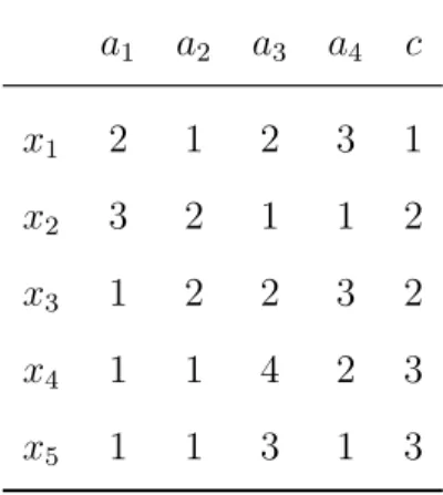
this study.Consider a data set in Table 2.1 which has five objects {x1, x2, x3,

x4, x5} , four attributes {a1, a2, a3, a4}, and one class index c. The domains

of values of a1, a2, a3, and a4 are {1, 2, 3}, {1, 2}, {1, 2, 3, 4}, and {1,

2, 3}, respectively. The domain of values of c is {1, 2, 3}. In most cases, the attributes in a data set usually consist of a mixture of qualitative and quantitative ones. In this study, all attributes are transformed into ordered

Table 2.1: A small data set a1 a2 a3 a4 c x1 2 1 2 3 1 x2 3 2 1 1 2 x3 1 2 2 3 2 x4 1 1 4 2 3 x5 1 1 3 1 3

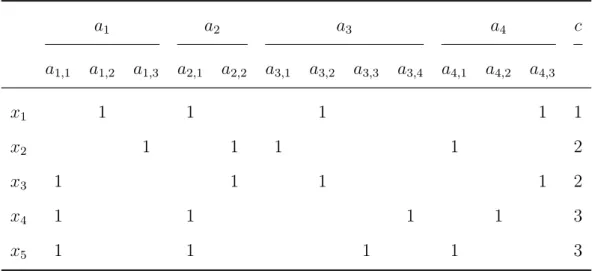
qualitative values. To induce rules for each class, first we convert Table 2.1

into another form presented by binary values in Table 2.2 , where aj,pis called

the p’th sub-attribute of j’th attribute. An object xi in Table 2.1 can then

be written as: xi = (ai1,1, a i 1,2, a i 1,3; a i 2,1, a i 2,2; a i 3,1, a i 3,2, a i 3,3, a i 3,4; a i 4,1, a i 4,2, a i 4,3; ci), where ai

j,p is 1 if aij (the value of ap of xi) equals p; otherwise, aij,p is 0. For

instance, x1 is expressed as

x1 = (0, 1, 0; 1, 0; 0, 1, 0, 0; 0, 0, 1; 1).

Notation 2.1. For a data set, which is characterized by m attributes. A

general form for expressing an object xi is written as:

xi = (ai1,1, . . . , a i 1,q1; a i 2,1, . . . , a i 2,q2; . . . ; a i m,1, . . . , a i m,qm; ci), (2.1)

where qm is the number of sub-attributes of the attribute am6, ci is the

class index of xi, and aij,p are sub-attribute values of xi, which are binary

6_{For convenience, the total number of sub-attributes of all attributes is denoted as q,}

Table 2.2: Binary presentation for the data set in Table 2.1 a1 a2 a3 a4 c a1,1 a1,2 a1,3 a2,1 a2,2 a3,1 a3,2 a3,3 a3,4 a4,1 a4,2 a4,3 x1 1 1 1 1 1 x2 1 1 1 1 2 x3 1 1 1 1 2 x4 1 1 1 1 3 x5 1 1 1 1 3

All blank cells are 0

values. An ai_j,p is 1 if ai_j = p; otherwise, ai_j,p is 0. Clearly, for each object xi,

∑

paij,p= 1 for all j. ¤

Notation 2.2. A general form of expressing a rule Rk,l_{, which is called the}

l’th rule for the class k, is expressed as:

Rk,l = (dk,l_1,1, . . . , dk,l_1,q 1; d k,l 2,1, . . . , d k,l 2,q2; . . . ; d k,l m,1, . . . , d k,l m,qm), (2.2)

where dk,l_j,p are binary variables specified as: if aj,p is an active sub-attribute

for Rk,l, then dk,l_j,p= 1; otherwise, dk,l_j,p= 0. ¤

Such a binary expression is useful in inducing rules with conjunctive and disjunctive forms.

Definition 2.1. (Support and Non-Violation) Given objects xi, xr, and a

rule Rk,l as represented in equations (2.1) and (2.2), respectively.

(i) Object xi belongs to a class k (i.e., ci = k): xi is called “supporting”

Rk,l _{, and R}k,l _{is called “supported by” x}

i, if ∑ paij,pd k,l j,p = 1 for all active attribute aj.

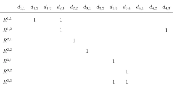
Table 2.3: Some rules for Table 2.1 d1,1 d1,2 d1,3 d2,1 d2,2 d3,1 d3,2 d3,3 d3,4 d4,1 d4,2 d4,3 R1,1 1 1 R1,2 _{1 1} R2,1 ₁ R2,2 1 R3,1 ₁ R3,2 ₁ R3,3 1 1

All blank cells are 0

(ii) Object xr does not belong to a class k (i.e., cr 6= k): xr is called

“non-violating” Rk,l_{, if}∑

pa

r

j,pd

k,l

j,p = 0 for any active attribute aj. ¤

Consider the example given in Table 2.1, Table 2.3 is a list of seven rules induced from Table 2.2. (The method of inducing rules are described in next

chapter). R1,1 _{is expressed by a binary vector as}

R1,1 = (0, 1, 0; 1, 0; 0, 0, 0, 0; 0, 0, 0).

Table 2.4 is the explanation of these rules. For instance, R1,1 means

“if (a1 = 2) and (a2 = 1), then the objects belong to class 1”.

The ignored attributes in R1,1 _{are a}

3 and a4; the active attributes are a1 and

a2 (in fact, the active sub-attributes are a1,2 and a2,1). This rule is supported

by object x1, since for these two active attributes, we have

∑

p=1...3

and

∑

p=1...2

a1_2,pd1,1_2,p = a1_2,1d1,1_2,1+ a1_2,2d1,1_2,2 = 1× 1 + 0 × 0 = 1.

And it is not violated by object x2, since for the active attribute a1, we have

∑

p=1...3

a2_1,pd1,1_1,p = a2_1,1d1,1_1,1+ a2_1,2d1,1_1,2+ a2_1,3d1,1_1,3 = 0× 0 + 0 × 1 + 1 × 0 = 0.

It is also not violated by objects x3 ,x4 and x5. Furthermore, two rules may

be integrated into a more general rule. For instance, R3,1 _{and R}3,2 _{can be}

combined as R3,3_{, expressed as}

R3,1∨ R3,2 = (0, 0, 0; 0, 0; 0, 0, 1, 0; 0, 0, 0)∨ (0, 0, 0; 0, 0; 0, 0, 0, 1; 0, 0, 0)

= (0, 0, 0; 0, 0; 0, 0, 1, 1; 0, 0, 0, )

= R3,3.

R3,3 means

“if (a3 = 3 or 4), then the objects belong to class 3”.

The meaning of the last three columns in Table 2.4 is explained in next chapter.

2.3

Notations and Variables Summary

Here is a summary of the notations and variables adopted in this chapter.

• xi: the object i in a data set.

• aj: the attribute j of objects.

• aj,p: the p’th sub-attribute of aj.

• c: the class index of objects.

T able 2.4: The explanation for rules in T able 2.3 activ e ignored supp orting non-violated accuracy supp ort compactness rule meaning sub-attributes attributes ob jects ob jects rate (AR ) rate (S R ) rate (C R ) R 1 ,1 if (a 1 = 2) ∧ (a 2 = 1), then c = 1 a1 ,2 , a2 ,1 a3 , a4 x1 x2 , x3 , x4 , x5 1 1 0.73 R 1 ,2 if (a 2 = 1) ∧ (a 4 = 3), then c = 1 a2 ,1 , a4 ,3 a1 , a3 x1 x2 , x3 , x4 , x5 1 1 0.73 R 2 ,1 if (a 2 = 2), then c = 2 a2 ,2 a1 , a3 , a4 x2 , x3 x1 , x4 , x5 1 1 1 R 2 ,2 if (a 3 = 1), then c = 2 a3 ,1 a1 , a2 , a4 x2 x1 , x4 , x5 1 0.5 1 R 3 ,1 if (a 3 = 3), then c = 3 a3 ,3 a1 , a2 , a4 x5 x1 , x2 , x3 1 0.5 1 R 3 ,2 if (a 3 = 4), then c = 3 a3 ,4 a1 , a2 , a4 x4 x1 , x2 , x3 1 0.5 1 R 3 ,3 if (a 3 = 3 ∨ 4), then g = 3 a3 ,3 , a3 ,4 a1 , a2 , a4 x4 , x5 x1 , x2 , x3 1 1 0.98 where “∧ ” means logic “AND” and “∨ ” means logic “OR”

• n: the total number of objects in a data set. • m: the total number of attributes in a data set. • q: the total number of sub-attributes of all attributes.

• qm: the number of sub-attributes of am.

• ai

j: the value of aj of xi.

• ai

j,p: the value of aj,p of xi.

• Rk,l_{: the l’th rule for the class k.}

• dk,l

j,p: a binary variable specified as: if aj,p is an active sub-attribute for

the rule Rk,l_{, then d}k,l

j,p = 1; otherwise, d

k,l

Chapter 3 Proposed Classification Methods

This chapter developes some essential propositions and a method of inducing rules such as those in Table 2.3. It also illustrates the proposed method with some examples.

3.1

Propositions

First, consider the following propositions:

Proposition 3.1. For objects xi (such ci = k), xr (such cr 6= k), and a

rule Rk,l as represented in equations (2.1) and (2.2), respectively, hk,l is

de-noted the number of ignored attributes by Rk,l_.

(i) Rk,l _{is supported by x} i , if ∑ j ∑ pa i j,pd k,l j,p= m− hk,l.

(ii) Rk,l _{is not violated by x}

r, if ∑ j ∑ pa r j,pd k,l j,p ≤ m − hk,l− 1.

Proof. From Definition 2.1, we have

(i) ∑_pai_j,pdk,l_j,p = 1 for all active attributes aj while Rk,l is supported by xi.

So it is clear that ∑_j∑_pai j,pd k,l j,p = m− hk,l. (ii) ∑_par j,pd k,l

j,p = 0 for any active attribute aj while Rk,l is not violated by

xr. So it is clear that ∑ j ∑ pa r j,pd k,l j,p ≤ m − hk,l− 1.

The proposition is then proven.

c1 = 1 and ∑ j ∑ p ai_j,pdk,l_j,p = (a1_1,1d1,1_1,1+ a1_1,2d1,1_1,2+ a1_1,3d1,1_1,3) + (a1_2,1d1,1_2,1+ a1_2,2d1,1_2,2) = (0× 0 + 1 × 1 + 0 × 0) + (1 × 1 + 0 × 0) = 2 = m− hk,l, R1,1 _{is supported by x} 1. Since c4 = 3 6= 1 and ∑ j ∑ p ar_j,pdk,l_j,p = (a4_1,1d1,1_1,1+ a4_1,2d1,1_1,2+ a4_1,3d1,1_1,3) + (a4_2,1d1,1_2,1+ a4_2,2d1,1_2,2) = (1× 0 + 0 × 1 + 0 × 0) + (1 × 1 + 0 × 0) = 1 ≤ m − hk,l _{− 1,}

x4 does not violate R1,1.

Proposition 3.2. Parameter hk,l _{is specified as h}k,l ₌∑

jλ k,l j , where λ k,l j ∈ {0, 1}. λk,l

j = 1 if attribute aj is ignored by a rule Rk,l; otherwise, λ

k,l

j =

0. The relationships between dk,l_j,p and λk,l_j are expressed as the following

inequalities: dk,l_j,p ≤ 1 − λk,l_j ,∀j, p, (3.1) 1− λk,l_j ≤∑ p dk,l_j,p,∀j, (3.2) λk,l_j ∈ {0, 1}. (3.3) Proof.

• If attribute aj is ignored by Rk,l, then dk,lj,p = 0 for all p,

∑

pd

k,l

j,p = 0

• If attribute aj is not ignored by Rk,l, then at least one dk,lj,p = 1, ∑ pd k,l j,p ≥ 1 and λ k,l j = 0.

The proposition is then proven.

Remark 3.1. For objects xi (such ci = k), xr (such cr 6= k), and a rule Rk,l,

here we introduce binary variables uk,l_i and vk,l_r :

(i) uk,l_i = 1, if xi supports Rk,l; otherwise uk,li = 0.

(ii) vk,l

r = 1, if xr does not violate Rk,l; otherwise vrk,l = 0. ¤

Proposition 3.3. Let M be a big positive number. For objects xi (such

ci = k), xr (such cr 6= k), and a rule Rk,l, there exit uk,li and vrk,l ∈ {0, 1}

which satisfy the following inequalities:

M (uk,l_i − 1) + m − hk,l ≤∑ j ∑ p ai_j,pdk,l_j,p ≤ m − hk,l _{+ M (1− u}k,l i ),∀i where ci = k, (3.4) ∑ j ∑ p ar_j,pdk,l_j,p ≤ m − hk,l− 1 + M(1 − v_rk,l),∀r where cr 6= k. (3.5) Proof. • If uk,l

i = 1, then equation (3.4) is equivalent to Case 1 of Proposition 3.1.

• If vk,l

r = 1, then equation (3.5) is equivalent to Case 2 of Proposition 3.1.

The proposition is then proven.

Consider a data set of n objects. Denote the number of objects belonging

to a specific class k as nk. The definitions of the accuracy rate, support rate

Definition 3.1. (Accuracy Rate) The accuracy rate of a rule Rk,l _{is specified} as ARk,l = 1 n− nk ∑ r where cr6=k v_rk,l. ¤

It means that if none of object xr (such cr 6= k) violates the rule (i.e., all

vk,l

r = 1), then the accuracy rate of the rule is 1. The binary parameter vrk,l

is specified in Remark 3.1.

Definition 3.2. (Support Rate) The support rate of a rule Rk,l _{is specified}

as SRk,l = 1 nk ∑ i where ci=k uk,l_i . ¤

If all objects xi (such ci = k) support the rule (i.e., all uk,li = 1), then its

support rate is 1. The binary parameter uk,l_i is specified in Remark 3.1.

Definition 3.3. (Compactness Rate) The compactness rate of a rule Rk,l is specified as CRk,l = 1 m ( hk,l+ 1− ∑ j ∑ pd k,l j,p− 1 q ) . ¤

It implies that if the most compact rule is the rule with only one active

sub-attribute (i.e., such ∑_j∑_pdk,l_j,p = 1), then CRk,l = 1. If different rules

have the same numbers of active sub-attributes, then the rule with larger ignored attributes number h is considered more compact than others. By the definition given here, the CR of a rule with larger h will be higher than

Remark 3.2.

(i) 0≤ ARk,l ≤ 1

(ii) 0≤ SRk,l _{≤ 1}

(iii) 0≤ CRk,l ≤ 1 ¤

The related AR, SR, and CR values for the example rules in Table 2.3

are listed in the last three columns of Table 2.4 . The CR value for R1,1 _is

computed as 1₄(2 + 1− 2₁₂−1) = 0.73. R2,1 is better than R2,2 since it has a

higher SR value. R3,3 has higher SR than do R3,1 and R3,2; however, R3,3 is

not as compact as R3,1 _{and R}3,2_.

3.2

Notations and Variables Summary

Here is a summary of the notations and variables adopted in this chapter.

• hk,l_{: the number of ignored attributes by R}k,l_.

• λk,l

j : a binary variable specified as: if aj is ignored by Rk,l, then λk,lj = 1;

otherwise, λk,l_j = 0.

• uk,l

i : a binary variable specified as: if xi supports Rk,l, then uk,li = 1;

otherwise, uk,l_i = 0.

• vk,l

r : a binary variable specified as: if xr dose not violate Rk,l, then

vk,l_r = 1; otherwise, uk,l_i = 0.

• M: a big positive number.

• nk_{: the number of objects which belong to the class k.}

• SRk,l_{: the support rate of R}k,l_.

• CRk,l_{: the compactness rate of R}k,l_.

3.3

Models for Inducing Rules

The program to induce a rule Rk,l _{is formulated as the following linear}

mul-tiobjective program: Max ARk,l Max SRk,l Max CRk,l Subject to: M (uk,l_i − 1) + m − hk,l ≤∑ j ∑ p ai_j,pdk,l_j,p ≤ m − hk,l _{+ M (1− u}k,l i ),∀i where ci = k, (C1) ∑ j ∑ p ar_j,pdk,l_j,p ≤ m − hk,l − 1 + M(1 − vk,l_r ),∀r where cr 6= k, (C2) dk,l_j,p ≤ 1 − λk,l_j , 1≤ j ≤ m, 1 ≤ p ≤ qj, (C3) 1− λk,l_j ≤∑ p dk,l_j,p, 1≤ j ≤ m, (C4) hk,l =∑ j λk,l_j , (C5) dk,l_j,p0 + dk,l_j,p0₊₂− 1 ≤ dk,l_j,p0₊₁, 1≤ p0 ≤ qj − 2, (C6) uk,l_i , vk,l_r , dk,l_j,p, λk,l_j ∈ {0, 1}, 1 ≤ i, j ≤ n, 1 ≤ j ≤ m, 1 ≤ p ≤ qj. (C7)

The objective of this program is to maximize AR, SR and CR simul-taneously, where constrainsts (C1) and (C2) come from Proposition 3.3, and constraints (C3)–(C5) come from Proposition 3.2. The purpose of con-straint (C6) is to avoid the discontinuity of active sub-attributes for the same

attribute. ARk,l_{, SR}k,l_{, and CR}k,l _{are specified in Definitions 3.1, 3.2, and}

3.3, respectively. This is a multiple criteria decision problem. There are three typical models for solving this multiobjective program:

(i) A constraint model, where two of the three objectives with lower bounds are assigned.

(ii) An aspiration model, where aspiration levels are set for the three ob-jectives.

(iii) A weighting model, where relative weights are assigned to the three objectives.

All these three models are reformulated below.

Model 3.1. (Specifying the lower bounds for AR and SR)

Max obj = CRk,l

Subject to: constraints (C1)–(C7), and

ARk,l ≥ AR,

SRk,l ≥ SR,

where AR and SR are constant, representing the lower bounds of ARk,l _and

SRk,l. ¤

Example 3.1. Take Table 2.3 for instance. The program to induce a rule

R1,l _{for class 1 using Model 3.1 is formulated below:}

Max CR1,l= 1 4 ( h1,l+ 1− ∑ j ∑ pd 1,l j,p 12 )

subject to: 5(u1,l₁ − 1) + 4 − h1,l ≤ d1,l_1,2+ d1,l_2,1+ d1,l_3,2+ d1,l_4,3 ≤ 4 − h1,l+ 5(1− u1,l₁ ), d1,l_1,3+ d1,l_2,2+ d1,l_3,1+ d1,l_4,1 ≤ 4 − h1,l− 1 + 5(1 − v₂1,l), d1,l_1,1+ d1,l_2,2+ d1,l_3,2+ d1,l_4,3 ≤ 4 − h1,l− 1 + 5(1 − v₃1,l), d1,l_1,1+ d1,l_2,1+ d1,l_3,4+ d1,l_4,2 ≤ 4 − h1,l− 1 + 5(1 − v₄1,l), d1,l_1,1+ d1,l_2,1+ d1,l_3,3+ d1,l_4,1 ≤ 4 − h1,l− 1 + 5(1 − v₅1,l), d1,l_1,p ≤ 1 − λ1,l₁ , for p = 1, 2, 3, (3.6) d1,l_2,p ≤ 1 − λ1,l₂ , for p = 1, 2, (3.7) d1,l_3,p ≤ 1 − λ1,l₃ , for p = 1, 2, 3, 4, (3.8) d1,l_4,p ≤ 1 − λ1,l₄ , for p = 1, 2, 3, (3.9) 1− λ1,l₁ ≤ d1,l_1,1+ d1,l_1,2+ d1,l_1,3, (3.10) 1− λ1,l₂ ≤ d1,l_2,1+ d1,l_2,2, (3.11) 1− λ1,l₃ ≤ d1,l_3,1+ d_3,21,l + d1,l_3,3+ d1,l_3,4, (3.12) 1− λ1,l₄ ≤ d1,l_4,1+ d1,l_4,2+ d1,l_4,3, (3.13) h1,l = λ1,l₁ + λ1,l₂ + λ1,l₃ + λ1,l₄ , (3.14) d1,l_1,1+ d1,l_1,3− 1 ≤ d1,l_1,2, (3.15) d1,l_3,1+ d1,l_3,3− 1 ≤ d1,l_3,2, (3.16) d1,l_3,2+ d1,l_3,4− 1 ≤ d1,l_3,3, (3.17) d1,l_4,1+ d1,l_4,3− 1 ≤ d1,l_4,2, (3.18) AR1,l = 1 5− 1(v 1,l 2 + v 1,l 3 + v 1,l 4 + v 1,l 5 )≥ AR,

SR1,l= 1 1u 1,l 1 ≥ SR, u1,l₁ , v₂1,l, v₃1,l, v1,l₄ , v₅1,l,d1,l_1,1, d1,l_1,2, d1,l_1,3, d1,l_2,1, d1,l_2,2, d_3,11,l, d1,l_3,2, d1,l_3,3, d1,l_3,4, d1,l_4,1, d1,l_4,2, d1,l_4,3, λ₁1,l, λ1,l₂ , λ1,l₃ , λ1,l₄ ∈ {0, 1}.

Solution. By pecifying AR, SR = 1, the optimal solutions obtained are

d1,l_1,2 = d1,l_2,1 = 1, and all others are d1,l_j,p = 0, u1,l₁ = v₂1,l= v1,l₃ = v1,l₄ = v₅1,l = 1,

λ1,l₁ = λ1,l₂ = 0, λ₃1,l = λ1,l₄ = 1, h1,l _{= 2. The objective value CR}1,l _is

1

4(2 + 1−

2−1

12 ) = 0.73. The rule is exactly the same as R

1,1 _{in Table 2.3 and}

Table 2.4. ¤

Example 3.2. Similarly, the model of inducing a rule R3,l _{for class 3 is}

formulated below:

Max CR3,l

subject to: equations (3.6)–(3.18) with changing superscripts 1, l to 3, l, and

5(u3,l₄ − 1) + 4 − h3,l ≤ d3,l_1,1+ d3,l_2,1+ d3,l_3,4+ d3,l₄₂ ≤ 4 − h3,l+ 5(1− u3,l₄ ), 5(u3,l₅ − 1) + 4 − h3,l ≤ d3,l_1,1+ d3,l_2,1+ d3,l_3,3+ d3,l_4,1 ≤ 4 − h3,l+ 5(1− u3,l₅ ), d3,l_1,2+ d3,l_2,1+ d3,l_3,2+ d3,l_4,3 ≤ 4 − h3,l− 1 + 5(1 − v₁3,l), d3,l_1,3+ d3,l_2,2+ d3,l_3,1+ d3,l_4,1 ≤ 4 − h3,l− 1 + 5(1 − v₂3,l), d3,l_1,1+ d3,l_2,2+ d3,l_3,2+ d3,l_4,3 ≤ 4 − h3,l− 1 + 5(1 − v₃3,l), AR3,l= 1 5− 2(v 3,l 1 + v 3,l 2 + v 3,l 3 )≥ AR, SR3,l= 1 2(u 3,l 4 + u 3,l 5 )≥ SR, v3,l₁ , v₂3,l, v3,l₃ , u3,l₄ , u3,l₅ ,d3,l_1,1, d3,l_1,2, d3,l_1,3, d3,l_2,1, d3,l_2,2, d_3,13,l, d3,l_3,2, d3,l_3,3, d3,l_3,4, d3,l_4,1, d3,l_4,2, d3,l_4,3, λ₁3,l, λ3,l₂ , λ3,l₃ , λ3,l₄ ∈ {0, 1}.

Solution. By specifying AR = SR = 1, the optimal solutions obtained are

d3,l_3,3 = d3,l_3,4 = 1, and all others are d3,l_j,p = 0, u3,l₄ = u3,l₅ = v₁3,l= v3,l₂ = v₃3,l = 1,

λ3,l₃ = 0, λ3,l₁ = λ₂3,l = λ3,l₄ = 1, h3,l = 3. The objective value CR3,l is

1

4(3 + 1−

2−1

12 ) = 0.98. The rule is exactly the same as R

3,3 _{in Table 2.3 and}

Table 2.4. ¤

Model 3.2. (Specifying the aspiration levels for AR, SR, and CR)

Max ARk,l + SRk,l + CRk,l

subject to: constraints (C1)–(C7), and

ARk,l ≥ AR,

SRk,l ≥ SR, CRk,l ≥ CR.

¤

Model 3.3. (Specifying the weights on AR, SR and CR)

Max wk,l_a ARk,l+ wk,l_s SRk,l+ wk,l_c CRk,l

subject to: constraints (C1)–(C7), where wk,l_a , wk,l_s and w_ck,lare the weighting

value of ARk,l_{, SR}k,l _{and CR}k,l_{, respectively.} ¤

In addition to inducing the best rule, we may also generate conveniently the second best, the third best, etc. rules.

Procedure 3.1. The solution procedure for Model 3.1 is: Step 1. Specify the AR and SR

Step 3. If no feasible solution exists

Step 3.1. Decrease AR or SR, and go to Step 3

Else

Step 3.2. A rule is obtained Step 4. If more rules are wanted,

Step 4.1. Add the solution obtained from Step 3.1 as a new constraint

for Model 3.1, then go to Step 2.

In the first iteration of Step 3.2 in Procedure 3.1, we get the global optimal rule for a specified class; and in the second iteration, we get the second optimal rule, and so on. Example 3.3 illustrates the solution procedure using Procedure 3.1.

Example 3.3. Take Example 3.2 for instance. Since u3,l₄ = u3,l₅ = 1 is the solutions of Example 3.2, if one more rule for class 3 is needed, we can add the following new constraint

u3,l₄ + u3,l₅ < 2

to the model of Example 3.2. This constraint prevents u3,l₄ = u3,l₅ = 1,

simul-taneously. There is no feasible solution after adding the above constraint. It

means that no more rule with AR3,l _{= SR}3,l _{= 1 can be induced. Then, we}

can decrease the acceptable level of AR or SR to get second best rules. Here,

we decrease SR to 0.5, and the solutions obtained are d3,l_3,2 = 1; all others are:

d3,l_j,p = 0, u3,l₄ = 0, u3,l₅ = v₁3,l = v₂3,l = v3,l₃ = 1, λ3,l₃ = 0, λ3,l₁ = λ3,l₂ = λ3,l₄ = 1,

R3,1 _{in Table 2.3, which is the second best rule for class 3. By adding the}

next constraint,

u3,l₅ < 1

to the model, the third best rule, exactly the same as R3,2 in Table 2.3, is

then obtained. ¤

3.4

Analysis of Models

For a data set having n objects and characterized by m attributes with q sub-attributes, the analysis of constraints and binary variables for inducing

a specific rule Rk,l _{is described below.}

• For each object, it needs either a constraint of (C1) or a constraint of (C2). So the instance of constraints of (C1) and (C2) is n.

• For each sub-attribute, it needs a constraint of (C3). So the instance of constraints of (C3) is q.

• For each attribute, it needs a constraint of (C4). So the instance of constraints of (C4) is m.

• There is only one instance of constraint (C5).

• The instance of constraints of (C6) depends on each qj. The worst case

is only one qj 6= 1 and the instance of constraints of (C6) is q − m − 2.

• The number of binary variables uk,l

i and vrk,l is n, since each object

needs a uk,l_i or vk,l

r .

• To represent a rule, it needs a binary variable dk,l

j,pfor each sub-attribute.

• The number of binary variables λk,l

j is m.

To sum up, the maximum number of constraints of (C1)–(C6) is n + 2q− 1

Chapter 4 Experiments

This chapter demonstrates the solution process of the proposed method by two practical data sets, the HSV (Highly Selective Vagotomy) patients and the European Barn Swallow, and compares the induction results with RST (or VPRS) and ID3.

4.1

The HSV Patients Data Set

The HSV patients data set is a clinical data set of F. Raszeja Mem. Hos-pital in Poland. HSV, also called proximal gastric vagotomy, is an effective method of treatment of duodenal ulcer, which consists of vagal denervating of the stomach area secreting hydrochloric acid (Dunn et al., 1980). This data set is composed of 122 patients with duodenal ulcer treated by HSV, as described by 11 pre-operating attributes. For more details about the data set, please see Appendix A. The patients are classified into four classes, ac-cording to a long-term result of HSV, and all evaluated by a surgeon in the modified Visick grading, following the definition of Goligher et al. (1978). Exact values of the considered quantitative attributes are translated into or-dered qualitative terms, i.e., “high,” “medium,” “low,” etc. This translation is due to some empirical norms defining intervals of attribute values corre-sponding to qualitative terms. The terms are then coded by numbers 1, 2, 3, etc., which create the domain of coded attributes. The norms adopted in the study are shown in Table 4.1 (Slowinski, 1992).

T able 4.1: Norms for attributes of the HSV data set Domain (co de) No. A ttribute [units] 1 2 3 4 5 Remarks a1 Gender male female a2 Age [y ears] ≤ 35 > 35 a3 Duration of disease [y ears] ≤ 0 .5 (0 .5 , 3] > 3 a4 Complication of ulcer none acute m ultiple p erforation p yloric haemorrhage haemorrhage in the past stenosis a5 HCL concen tration [mmol HCL/100ml] ≤ 2 (2 , 4] > 4 basic secretion a6 V olume of gastric juice p er 1h [ml] ≤ 70 (70 , 150] > 150 a7 V olume of residual gastric juice [ml] ≤ 50 (50 , 100] > 100 a8 Basic acid output (BA O) [mmol HCL/h] ≤ 2 (2 , 3] > 3 a9 HCL concen tration [mmol HCL/100ml] ≤ 10 (10 , 15] > 15 secretion stim ulated a10 V olume of gastric juice p er 1h [ml] ≤ 100 (100 , 250] > 250 b y histamine a11 Maximal acid output [mmol HCL/h] ≤ 15 (15 , 25] (25 , 40] > 40 This table is extracted from Slo winski (1992).

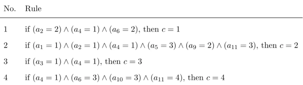
Table 4.2: The best rule for each class of HSV found by ROSE2 No. Rule 1 if (a2 = 2)∧ (a4 = 1)∧ (a6= 2), then c = 1 2 if (a1 = 1)∧ (a2 = 1)∧ (a4= 1)∧ (a5 = 3)∧ (a9 = 2)∧ (a11= 3), then c = 2 3 if (a3 = 1)∧ (a4 = 1), then c = 3 4 if (a4 = 1)∧ (a6 = 3)∧ (a10= 3)∧ (a11= 4), then c = 4

4.1.1 Rules Induced by RST and ID3

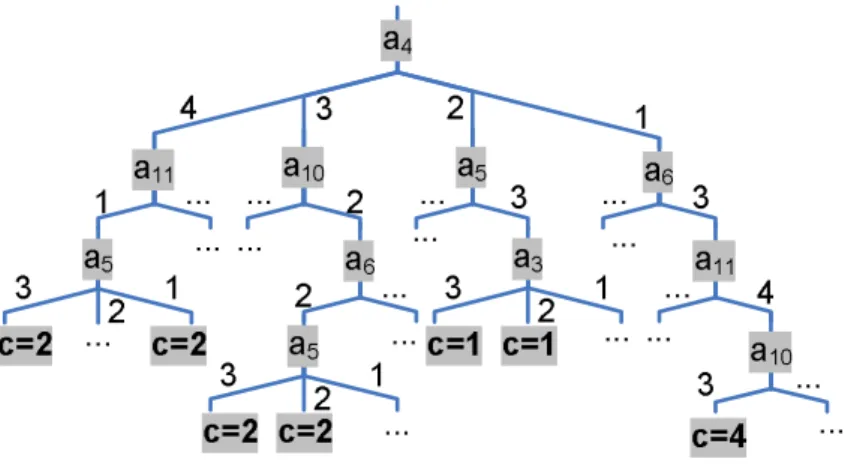
Here, we use a software tool named ROSE2 (Rough Sets Data Explorer)(Predki et al., 1998; Predki and Wilk, 1999) to induce rules by RST. The compu-tations of ROSE2 are based on rough-set fundamentals. Table 4.2 lists the best rule for each class found by ROSE2.

Figure 4.1 is the partial HSV classification tree by ID3, which only lists

the best path for each class. For example, from the branch a4 = 1, a6 = 3,

a11= 4 and a10= 3, the leaf c = 4 is reached. It means that

“if (a4 = 1) and (a6 = 3) and (a11 = 4) and (a10= 3),

then the objects belong to class 4”.

4.1.2 Rules Induced by the Proposed Method

To simplify the presentation, we utilize Model 3.1 to induce rules where the accuracy rate is fixed at 100%. The used model is as follows:

Max CRk,l

subject to: constraints (C1)–(C7), and

a6 1 3 ... ... 3 c=4 2 3 ... 4 ... 3 2 ... a4 a11 a10 ... a5 4 a10 a6 2 a11 1 ... ... ... ... ... ... ... ... a3 2 3 1 c=1 c=1 ... a5 2 3 1 c=2 c=2 ... a5 2 3 1 c=2 ... c=2

Figure 4.1: A partial ID3 decision tree for HSV data set.

SRk,l ≥ α,

where CRk,l is to be maximized with restrictions that ARk,l = 1 and SRk,l ≥

α. α is a parameter value. The best rule found and the second best rules for

each class are listed in Table 4.3. R1,1 _{means the best rule for class 1, and}

R1,2 _{is the second best rule for class 1. R}1,1 _{is found by specifying α =} 19

79

(there is no feasible solution for α > 19₇₉), which means

“if (a2 = 2) and (a4 = 1 or 2 or 3) and (a9 = 3),

then the objects belong to class 1”.

The rule R1,1 _{is supported by 19 objects. They are x}

1, x4, x9, x11, x15, x19,

x25, x27, x46, x57, x61, x71, x83, x88, x94, x104, x106, x111, and x117. Its support

rate is SR1,1₌ 19

79 = 0.24 . There are eight attributes ignored and five active

sub-attributes in R1,1_{, so its compactness rate is CR}1,1 ₌ 1

11(8 + 1−

5−1 34 ) =

0.81. The second best rule R1,2 _{is conveniently induced by adjusting α =} 17

79

and adding the following new constraint to Model 3.1.

u1,2₁ + u1,2₄ + u1,2₉ + u1,2₁₁ + u1,2₁₅ + u1,2₁₉ + u1,2₂₅ + u1,2₂₇ + u1,2₄₆ + u1,2₅₇ + u1,2₆₁ + u1,2₇₁ + u1,2₈₃ + u1,2₈₈ + u1,2₉₄ + u1,2₁₀₄+ u1,2₁₀₆+ u1,2₁₁₁+ u1,2₁₁₇ < 19.

The solution is R1,2_{, which means}

“if (a4 = 2) and (a9 = 2 or 3), then the objects belong to class 1”

with CR1,2 = 0.90 and SR1,2 = 0.16. In the same processes, the best rules for

remaining three classes are obtained. The SR of the best rules for classes 2, 3, 4 are 0.22, 0.38,0.23, respectively, and CR are 0.72, 0.81, 0.63, respectively

4.1.3 Comparison of Results

Here, we compare the proposed method with ROSE2 and ID3. Table 4.3 lists the best rules found by the three methods. All the rules listed here are 100%

accuracy. For class 1, R1,1 _{with CR}1,1 _{= 0.81 and SR}1,1 _{= 0.24 and R}1,2 _with

CR1,2 = 0.90 and SR1,2 = 0.16 are the best and second best rules found by

the proposed method, respectively. R1,3 with CR1,3 = 0.81 and SR1,3 = 0.16

is the best rule that can be found by ROSE2. It is worse than R1,1 _and

R1,2_{. R}1,4 _{with CR}1,4 _{= 0.81 and SR}1,4 _{= 0.15, the best rule that can be}

found by ID3, is even worse than R1,3. For class 2, R2,1 with CR2,1 = 0.72

and SR2,1 = 0.22, the best rule found by both the proposed method and

ID3, is better than R2,2 _{with CR}2,2 _{= 0.53 and SR}2,2 _{= 0.22, the best rule}

that can be found by ROSE2. Consider class 3, R3,1 _{with CR}3,1 _{= 0.81 and}

SR3,1 = 0.38 is the best rule found by the proposed method. Although R3,2

with CR3,2 _{= 0.91 and SR}3,2 _{= 0.25 is the second best rule found by the}

proposed method, it is the best rule that can be found by ROSE2. R3,3 _with

CR3,3 _{= 0.81 and SR}3,3 _{= 0.25, the best rule that can be found by ID3, is}

worse than R3,2. Similarly, R4,1, the best rule found by proposed method, is

T able 4.3: Comparison of the prop osed metho d, R OSE2 and ID3 for the HSV data set. Class Used Induced Meaning of rule AR S R C R Supp orting ob jects metho ds rule 1 Prop osed R 1 ,1 if (a 2 = 2) ∧ (a 4 = 1 ∨ 2 ∨ 3) ∧ (a 9 = 3), 1 0.24 0.81 x1 , x4 , x9 , x11 , x15 , x19 , x25 , x27 , x46 , x57 , x61 , x71 , then c = 1 x83 , x88 , x94 , x104 , x106 , x111 , x117 Prop osed R 1 ,2 if (a 4 = 2) ∧ (a 9 = 2 ∨ 3), then c = 1 1 0.16 0.90 x2 , x6 , x7 , x8 , x16 , x46 , x47 , x52 , x56 , x57 , x88 , x116 , x117 R OSE2 R 1 ,3 if (a 2 = 2) ∧ (a 4 = 1) ∧ (a 6 = 2), then c = 1 1 0.16 0.81 x1 , x9 , x19 , x25 , x31 , x48 , x67 , x83 , x93 , x97 , x106 , x114 , x115 ID3 R 1 ,4 if (a 3 = 2 ∨ 3) ∧ (a 4 = 2) ∧ (a 5 = 3), then c = 1 1 0.15 0.81 x2 , x6 , x7 , x8 , x16 , x46 , x47 , x52 , x56 , x88 , x116 , x117 2 Prop osed / R 2 ,1 if (a 4 = 3) ∧ (a 5 = 2 ∨ 3) ∧ (a 6 = 2) ∧ (a 10 = 2), 1 0.22 0.72 x12 , x45 , x62 , x110 ID3 then c = 2 R OSE2 R 2 ,2 if (a 1 = 1) ∧ (a 2 = 1) ∧ (a 4 = 1) ∧ (a 5 = 3) ∧ 1 0.22 0.53 x87 , x90 , x103 , x120 (a 9 = 2) ∧ (a 11 = 3), then c = 2 3 Prop osed R 3 ,1 if (a 3 = 2) ∧ (a 9 = 1) ∧ (a 11 = 2 ∨ 3), then c = 3 1 0.38 0.81 x43 , x79 , x109 Prop osed / R 3 ,2 if (a 3 = 1) ∧ (a 4 = 1), then c = 3 1 0.25 0.91 x5 , x56 R OSE2 ID3 R 3 ,3 if (a 4 = 4) ∧ (a 5 = 1 ∨ 3) ∧ (a 11 = 1), then c = 3 1 0.25 0.81 x13 , x24 4 Prop osed R 4 ,1 if (a 1 = 2) ∧ (a 2 = 2) ∧ (a 3 = 3) ∧ (a 5 = 3) ∧ 1 0.23 0.63 x18 , x75 , x107 (a 6 = 1), then c = 4 Prop osed R 4 ,2 if (a 6 = 3) ∧ (a 9 = 3) ∧ (a 10 = 3), then c = 4 1 0.15 0.81 x39 , x75 R OSE2 / R 4 ,3 if (a 4 = 1) ∧ (a 6 = 3) ∧ (a 10 = 3) ∧ (a 11 = 4), 1 0.15 0.72 x39 , x75 ID3 then c = 4 The rules are rank ed b y S R then C R .

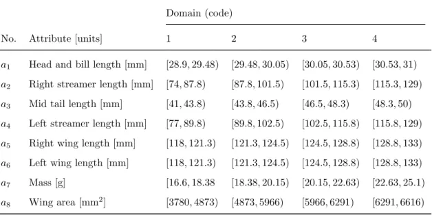
Table 4.4: Norms for attributes of the European barn swallow data set

Domain (code)

No. Attribute [units] 1 2 3 4

a1 Head and bill length [mm] [28.9, 29.48) [29.48, 30.05) [30.05, 30.53) [30.53, 31)

a2 Right streamer length [mm] [74, 87.8) [87.8, 101.5) [101.5, 115.3) [115.3, 129)

a3 Mid tail length [mm] [41, 43.8) [43.8, 46.5) [46.5, 48.3) [48.3, 50)

a4 Left streamer length [mm] [77, 89.8) [89.8, 102.5) [102.5, 115.8) [115.8, 129)

a5 Right wing length [mm] [118, 121.3) [121.3, 124.5) [124.5, 128.8) [128.8, 133)

a6 Left wing length [mm] [118, 121.3) [121.3, 124.5) [124.5, 128.8) [128.8, 133)

a7 Mass [g] [16.6, 18.38 [18.38, 20.15) [20.15, 22.63) [22.63, 25.1)

a8 Wing area [mm2] [3780, 4873) [4873, 5966) [5966, 6291) [6291, 6616)

4.2

The European Barn Swallow Data Set

The European barn swallow (Hirundo rustica) data set was obtained by trapping individual swallows in Stirlingshire, Scotland, between May and July 1997 (Beynon and Buchanan, 2003). This data set contains 69 swallows, which were described by eight attributes. For more details about the data set, please see Appendix B. The birds are classified by gender of each bird. The norms of attributes of the swallow data set are shown in Table 4.4.

4.2.1 Rules Found by VPRS and ID3

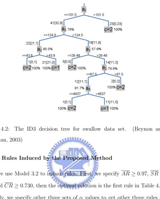
The rules found by VPRS (variable precision rough sets), a variant of RST, as shown in Beynon and Buchanan (2003), are listed in Table 4.5, where AR, SR and CR values are computed by this study.

The rules found by ID3, also appearing in Beynon and Buchanan (2003), are listed in Figure 4.2. Each terminal node of the decision tree classifies all its associated objects correctly into the identified decision class. At each node,

Table 4.5: Rules for swallow data set found by VPRS Rule AR SR CR 1 if (a2 = 1∨ 2) ∧ (a5 = 1∨ 2) ∧ (a6 = 1∨ 2), then c = 1 0.97 0.66 0.730 2 if (a1 = 3∨ 4) ∧ (a2 = 1∨ 2), then c = 1 1 0.16 0.863 3 if (a2 = 3∨ 4), then c = 2 1 0.72 0.996 4 if (a1 = 1∨ 2) ∧ (a5 = 3∨ 4) ∧ (a6 = 3∨ 4), then c = 2 0.97 0.31 0.730

The rules are extracted from Beynon and Buchanan (2003) where AR, SR and CR are computed by this study.

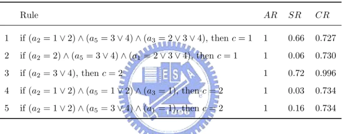
Table 4.6: Some better rules for swallow data set found by ID3

Rule AR SR CR 1 if (a2= 1∨ 2) ∧ (a5= 3∨ 4) ∧ (a3= 2∨ 3 ∨ 4), then c = 1 1 0.66 0.727 2 if (a2= 2)∧ (a5= 3∨ 4) ∧ (a1= 2∨ 3 ∨ 4), then c = 1 1 0.06 0.730 3 if (a2= 3∨ 4), then c = 2 1 0.72 0.996 4 if (a2= 1∨ 2) ∧ (a5= 1∨ 2) ∧ (a3= 1), then c = 2 1 0.03 0.734 5 if (a2= 1∨ 2) ∧ (a5= 3∨ 4) ∧ (a1= 1), then c = 2 1 0.16 0.734

information is given for the objects associated with it. From the root (top)

node the left-hand branch is defined by a2 ≤ 101.5 with 41[32, 9] representing

41 objects satisfying this criteria. Of them, 32 objects have class value ‘1’ and nine objects have class value ‘2’. Also shown to the right of every node box is the majority proportion of the objects in a same decision class. Continuing the same example as before, 32/41 = 0.780 is the highest proportion of the objects at that node to the same decision class. Since this is a complete tree, a terminal node is identified when the associated majority proportion value

equals 100%. Figure 4.2 can be expressed in ”If· · · Then · · · ” form as shown

a2 >101.5 c=2 23[0,23] 100% <=101.5 a5 >124.5 <=124.5 78% a1 a3 c=2 c=1 >43.8 <=43.8 1[0,1] 21[21,0] 57.9% 19[11,8] 22[21,1] >29.48 <=29.48 c=2 5[0,5] 100% 100% 100% a2 14[11,3] 95.5% 78.6% a8 100%c=2 2[0,2] >87.5 <=87.5 12[11,1] 91.7% >4837 <=4837 c=2 c=1 1[0,1] 11[11,0] 100% 100% 41[32,9]

Figure 4.2: The ID3 decision tree for swallow data set. (Beynon and

Buchanan, 2003)

4.2.2 Rules Induced by the Proposed Method

Here, we use Model 3.2 to induce rules. First, we specify AR ≥ 0.97, SR ≥

0.66 and CR ≥ 0.730, then the optimal solution is the first rule in Table 4.7.

Similarly, we specify other three sets of α values to get other three rules as listed in Table 4.7.

Table 4.7: Rules for swallow data set found by the proposed method

Rule AR SR CR AR SR CR 1 if (a2= 1∨ 2) ∧ (a5= 1∨ 2), then c = 1 0.97 0.66 0.730 0.97 0.66 0.863

2 if (a1= 4)∧ (a2= 1∨ 2), then c = 1 1 0.16 0.863 1 0.16 0.867

3 if (a2= 3∨ 4), then c = 2 1 0.72 0.996 1 0.72 0.996

4.2.3 Comparison of Results

Compare Table 4.7 with Table 4.5 and Table 4.6 to know that the proposed method can induce rules with better or equivalent values of AR, SR and CR. For example, the aspiration levels AR, SR and CR of the four rules in Table 4.7 are set as equal to the corresponding AR, SR and CR in Table 4.5. The results show that the first, second and fourth rules in Table 4.7 are better than the corresponding rules in Table 4.5, and the third rule in both table are the same. In fact, the proposed method can induce optimal solutions while ROSE2 and ID3 may find only feasible solutions.

Chapter 5 Implementation

MCOCR (Multiple Criteria Optimal Classification Rules) is a software tool implementing the models proposed by this study. It is currently a proto-type. MCOCR is developed by DELPHI 7.0 and runs on the Microsoft

WindowsXP operating system. The computing kernel behind MCOCR is LINGO 9.0. MCOCR gathers input data and relative parameters from users

in order to generate a corresponding LINGO program, then calls LINGO to solve such a program. Finally, MCOCR interprets the results returned by

LINGO into rules form.

Before starting MCOCR, an input data file must be prepared. The input data file contains the data set to be induced rules. In addition, the input data file also contains some meta information about the data set itself. So it must follow the input data file format, otherwise MCOCR cannot work properly. For more detail about input data file format, please see Appendix C.

When starting MCOCR, you will see the window shown in Figure5.1. There are five tags in the window:

• Model: for choosing which model (i.e., Model 3.1, 3.2 or 3.3) used • Parameter: for inputting parameters that MCOCR needs

• Origin Data: for showing contents of an input data file

• Program: for showing the LINGO model generated by MCOCR • Result: for showing the rules induced by MCOCR

So, the fist thing is to decide what model used. Here, Model 3.1 is used as an example. After chosen a model, the user must input some related parameters. There are some steps to induce rules.

• Select an input data file (Figure 5.1). After chosen an input data file, the “Origin Data” tag appears (Figure 5.2). Click the tag, contents of the input file will be displayed on the window (Figure 5.3).

• Select an objective, for instance, “max CR” (Figure 5.4).

• Specify lower bounds, for instance, “AR” and “number of supporting objects” (Figure 5.4).

• Specify the class value to classify (Figure 5.4).

• Generate LINGO program (Figure 5.4). While LINGO program gen-erated, the “Program” tag appears (Figure 5.5). Click the tag, contents of the generated LINGO program will be displayed on the window (Figure 5.6).

• Induce rules(Figure 5.7). The “Result” tag will appear while a rule generated and generated rules will be displayed on the window (Fig-ure 5.8).

• Induce next rules if needed (Figure 5.9). The rules will display on the window after previous rules (Figure 5.10).

Figure 5.1: Step1: Click ”Select Data File” button to select an input data file

Figure 5.3: Click ”Origin Data” tag, the contents of the input file will be displayed on the window.

Figure 5.4: Select an objective. The ”max CR” is chosen, here. Specify Lower Bounds. The AR is specified as 1 and the number of supporting objects is specified as 3, here. Specify the class to classify. Here is 2. Click ”Generate Program” button to generate LINGO program.

Figure 5.5: After ”Generate Program” button clicked, the ”Program” tag appears.

Figure 5.6: Click ”Program” tag, the contents of the generated Lingo pro-gram will be displayed on the window.

Figure 5.7: Step 6: Click ”Induce Rule” button to start inducing rules.

Figure 5.8: The ”Result” tag will appear while a rule generated and generated rules will be displayed on the window.

Figure 5.9: Click ”Induce Next Rule” button to induce another rule.

Chapter 6 Discussions and Remarks

6.1

Discussions

This study develops a multiple criteria mixed 0-1 linear programming model to induce rules. Some advantages of the proposed method are listed below:

(i) Solution quality: The rules obtained by the proposed method are glob-ally optimal solutions, but the rules obtained by RST or ID3 may just be feasible solutions.

(ii) Multiple criteria: Three criteria accuracy rate, support rate, and com-pact rate are considered to be maximized simultaneously.

(iii) Constraints: The proposed method is conveniently to add other con-straints to fit requirements, but it is difficult to do in RST and ID3 methods.

Although the proposed method is applied in biology and medicine infor-matics, it can apply in a variety of research and application areas.

6.2

Remarks

Although the adventages mentioned above, there are some limitations of proposed method, which are the future works of this study.

The number of binary variables uk,l_i and vk,l

r is direct propotion to the

number of obejcts n in such data set. While the number of objects become large, the computation time will increase, seriously. The numbers of binary

and sub-attributes q, respectively, but this is a relatively minor problem since the numbers of attributes and sub-attributes are not very large in most cases.

So, how to discrease the number of uk,l_i and v_rk,l is a major issue for future