Breast Cancer Classification and Biomarker Discovery on Microarray Data Using Genetic Algorithms and Bayesian Classifier

Breast Cancer Classification and Biomarker Discovery on Microarray

Data Using Genetic Algorithms and Bayesian Classifier

Tsun-Chen Lin

Department of Computer Science and Engineering, Dahan Institute of Technology

lintsunc@ms01.dahan.edu.tw

Abstract-

Keywords: Genetic algorithm, Bayesian classifier,

microarray, classification, breast cancer.

1. Introduction

Breast cancer is one of the most important diseases affecting women in the world. Traditionally, a thorough evaluation for breast cancer and its subtypes include an examination of both prognostic and predictive factors. Prognostic factors like tumor size, auxiliary lymph node status, and tumor grade, and predictive factors like estrogen receptor (ER), progesterone receptor (PR), and HER2/neu considered in the routine examination of breast cancer patients, however, cannot ultimately distinguish those patients who have identical traditional diagnosis and how they may respond to different therapies. Because of this, recent researches suggest that the classification of tumors based on gene expression patterns on microarray data may serve as a medical application in the form of diagnosis of the disease as well as a prediction of clinical outcomes in response to treatments [9][15].

The analysis of gene expression profiles, which serve as molecular signatures for tumor/cancer

classification, have become a highly challenging area of research in bioinformatics. In general, the classification of microarray data may be thought as a problem consisting of two tasks: (1) gene selection and (2) classification. Gene selection is the recognition of informative genes from thousands of highly correlated gene expression profiles for sample classification. Classification requires the construction of a model, which processes input patterns representing objects, and predicts the class or category associated with the objects under consideration. In the past few years, algorithms [1][2][3][8][18][20] with rank-based gene selection schemes have been applied to 2-class or 3-class classification problems based on gene expression data, and most have achieved 95%-100% classification accuracy. When these methods suggest that genes that classify tumor types well might serve as prognosis markers, the classification of microarrays for biomarker discovery becomes an important topic in bioinformatics. In fact, while there are certainly more types of cancers, if we expand the tumor classification problem to multiple tumor classes (more than 5), this problem will become more difficult because the dataset will contain more classes, but only a small number of samples [6][7][17]. Several recent papers [4][16][19] have addressed this problem and they concluded that many currently used approaches, relying on rank-based gene selection methods, may select redundant genes with highest scores in gene selection process. This implies that informative genes that are individually not discriminatory but complimentary to each other for discriminant analyses may not be selected. As one of the future directions discussed in the paper of Li et al. [19], the authors suggested designing a feature selection method to consider the correlations between features in microarray classification problem. Therefore, genetic algorithms, one of the wrapper-based gene selection methods, were applied to microarray classification problems to search optimal groups of co-working genes in

)} ( log 2 log )' ( ) ( { max arg ) ( 1 k p e e e f k k k k k + ∑ − − ∑ − − = v _μ − v _μ v (4) chromosomes, and evaluated the effectiveness of

the features selected on the actual classification task itself [5][11][12][13][22].

Since GAs with these computational models already shown their superiority to improve the prediction accuracy of classifiers, in this paper, we will combine GA and a Bayes classifier for breast cancer classification. The advantage to utilize Bayes classifiers is because Bayes classifiers only require a small amount of training data to estimate the parameters (means and variances of the variables) necessary for classification. This is why we attempt to develop a discriminant function based on a covariance matrix to consider the interactions between genes and see how these relationships may affect classification results. Consequently, our approach exhibits an excellent performance not only in classification accuracy but also at identifying genes that are already known to be cancer associated.

whereμ and k ∑k denote the class mean vector

and the covariance matrix of class k. In order to calculate−(ev−μ_k)∑_k−1(ev−μ_k)', the main quantity of Equation (4), we may define the class density of each class has the same common covariance matrix, ∑k =∑ [14], and therefore the classification rules can be rewritten as

} )' ( ) ( { max arg ) ( _{= − −μ ∑}−1 _−μ e e e f v _k v _k v (5) where

∑

And T is the number of all training samples. For example, in the training stage, if we want to predict the class of a query sample of class k, the output of the classification rule should be the winning class of k. Otherwise the sample is misclassified. In addition, the preceding rule can also be used to predict the class label of a novel sample, since there exists only one class deserving the maximum posterior probability.

2. Methods

2.1 Bayesian Classifier

For sample classification, assume that we are given a dataset in which D = {(evj,l ), for j=1…m}

is a set of m number of samples with well-defined class labels for multi-class prediction task. The feature vector,ev = (e₁,e₂,..., e_n) , denotes the vector of samples describing expression level of n number of predictive genes, l

∈

the class label associated with ev and q is the

number of classes. To view our prediction tasks as a Bayesian decision problem, our method uses Equation (1) to express the posterior probability of class k given sample feature vectorev as

) ( ) ( ) | ( ) | ( e p k p k e p e k P _v v v = (1)

where p v(e|k)is the class conditional densities, and is the class priors. For classification, the Bayes rule used to predict the class of a sample

) (k p

ev by that with highest posterior probability can be

defined as 2.2. Genetic Algorithms ) | ( max arg ) (e P k e f v = _k v (2)

In order to select an optimal subset of features from a large feature space to minimize the classification errors, we employ the GA approach. The genetic algorithms are adopted from Ooi and Tan [5], with toolboxes of two selection methods including stochastic universal sampling (SUS) and roulette wheel selection (RWS). In addition, two tuning parameters, Pc: crossover rate and Pm:

mutation rate, are used to tune one-point (OP) and uniform (Uni) crossover operations to evolve the population of individuals in the mating pool. The format of chromosomes used to carry subsets of genes are defined by the string Si, Si = [n g1 g2 … gnmax], where n is a randomly assigned value

ranging from nmin to nmax and g1 g2 … gnmax, are the

indices of nmax genes corresponding to a dataset. In

our experiments, every chromosome will be used to express a Dn×m dataset which is used by the

classifier to decide to which of a fixed set of classes that sample belongs. In training stage, we will try as many chromosomes as possible to choose the optimal gene subset by scoring those chromosomes using the fitness function of f (Si) =

(1 – Et) ×100, where Et means the training error

rate of Leave-One-Out Cross Validation (LOOCV ) test. Moreover, the optimal feature set will also be examined by independent tests. In order to have an Since the feature values of ev are given, and is

effectively constant. A widely used way to represent Equation (2) as a Bayesian decision rule for classification can be modified as

) ( log ) | ( log max arg ) (e p e k p k f v = _k v + (3)

Note that when the densities p v(e|k) are multivariate normal, Equation (3) will take the form as

unbiased estimation of initial gene pools, our algorithms will set 100 gene pools to run following steps.

Step 1: For each gene pool, the evolution process

will go 100 generations and each generation will evolve 100 chromosomes in which the size of genes will range from nmin=20 to nmax=30.

Step2: According to the gene indices in each

chromosome, only the first n genes are picked from g1, g2… gnmax to form sample patterns for

classification. In other words, the dataset is then represented by a matrix Dn×m form with rows for

the n genes and columns for the m samples.

Step 3: In order to estimate the fitness score for

each chromosome, the training dataset Dn×P of P

training samples and the test dataset Dn×m-P of

n×m-P test samples are fed into the following program to evaluate how well those samples can be correctly classified.

1. FOR each chromosome Si

2. FOR each training sample with class label lj 3. Build up discriminant model with

remainingtraining samples for LOOCV tests 4. IF (l_j ≠ f(er_j))

5. XtError = XtError + 1 // sample misclassified 6. END FOR

7. Et = XtError / Total training samples 8. Fitness[Si]= (1-Et) × 100

9. END FOR

10. Findmax (Fitness) // best chromosome

Step 4: By calculating the fitness value of

classification accuracy in a generation, the optimal fitness value will be stored to provide feedback on the evolution process of GA to find the increasing fit of chromosomes in the next generation.

Step 5: Repeat the process from Step 2 for the

next generation until the maximal evolutionary epoch is reached.

3. Dataset

The breast cancer gene expression profiles were measured with 7937 spotted cDNA sequences among the 85 samples with 6 different classes of breast tumor that were supplied by Stanford Microarray Database. This dataset was first studied by Sorlie et al. [21] and can be downloaded from http://genome-www5.stanford.edu/. The dataset originally contained six subclasses including basal-like (14 samples), ERBB2+ (11 samples), normal basal-like (13 samples), luminal subtype A (32 samples), luminal subtype B (5 samples), and luminal subtype C (10 samples). In our experiments, the dataset was divided into a training set of 57 samples and a test set of 28 samples so that the training errors could be calculated by

LOOCV tests, and so that a model could be built with the training data to present the results of predicting the label of unseen data. The training/test datasets with the ratio of 2:1 include gene expression profiles of 10/4 basal-like, 7/4 ERBB2+, 9/4 normal basal-like, 21/11 luminal subtype A, 3/2 luminal subtype B, and 7/3 luminal Subtypes c.

3.1 Data Preselection

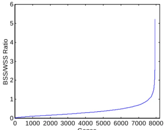
Since most genes in a microarray are irrelevant to class distinction, in order to select genes with the best discrimination ability used by our classifier, we follow the criterion established by Dudoit et al. [16] to filter out genes that are strongly correlated to class distinction using between group to within group sum of squares ratios (BSS/WSS) for data dimensionality reduction. As indicated by Figure 1 This figure suggests that only a fraction of genes show strong expression differentiation among tumor types and would be helpful for subsequent classification purpose. In our case, we decided to choose 2000 genes with the highest BSS/WSS ratio for our experiments. This means the dataset finally had 2000 genes × 85 samples remaining in the matrix and the BSS/WSS ratio for the dataset ranges from 0.48 to 5.23. 0 1000 2000 3000 4000 5000 6000 7000 8000 0 1 2 3 4 5 6 Genes B SS/ W S S R a ti o

Figure 1. Genes sorted by BSS/WSS ratio.

4. Experiments and Results

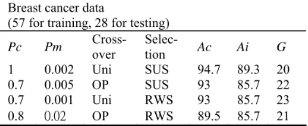
In Table 1, we have tried many groups of GA parameters for possible prediction performances. The best prediction accuracy was achieved using the Uniform crossover and SUS selection strategy of GA. The best predictor set obtained from our method exhibits LOOCV accuracy (Ac) of 94.7% in comparison with the cross validation success rate of 86% by the BSS/WSS/SVM [10]. Even in diagnosing blind test samples our method needed only 20 predictive genes to produce independent test accuracy of 89.3%, whereas BSS/WSS/SVM only performed cross validation tests and needed

hundreds of predictive genes.

Table 1. Accuracy measured in percentage.

Breast cancer data

(57 for training, 28 for testing)

Pc Pm Cross- _over Selec- _tion Ac Ai G 1 0.002 Uni SUS 94.7 89.3 20 0.7 0.005 OP SUS 93 85.7 22 0.7 0.001 Uni RWS 93 85.7 23 0.8 0.02 OP RWS 89.5 85.7 21 In Figure 2, we listed the best case of experiments and demonstrated the convergence of our method. In the running of above program, the chromosome with the best fitness, chosen from the simulation to arrive at the optimal operation will be based on the idea that a classifier must work well on the training samples, but also work equally well on previously unseen samples. Therefore, the optimal individuals of each generation were sorted in ascending order by the sum of the error number on both tests. The smallest number then determines the chromosome that contains predictive genes and the number of genes needed in the classification as well as gives the classification accuracy obtained by our methods. 0 10 20 30 40 50 60 70 80 90 100 0 0.1 0.2 0.3 0.4 0.5 0.6 0.7 0.8 0.9 1 Generations A ccur a cy Training Testing Pc=1 Pm=0.002 Crossover=Uniform Selection=SUS

Figure 2. This figure plots the degree of training accuracy (top line) and testing accuracy (bottom line) obtained from the best run out of 100 individual runs.

5. Predictive Genes

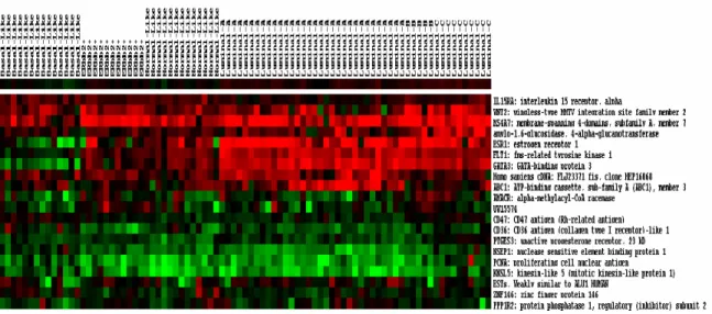
For the best gene subset found by our method, the heatmap of Figure 3 identifies the filtered 20 genes to reveal potential tumor subclasses and their associated biomarkers. Despite the lack of a broader investigation of these genes, below we list some informative genes and describe their

relationships with breast cancers.

(1). IL15RA is a proinflammatory molecule which is associated with tumor progression in head and neck cancer.

(2). WNT2 is one of proto-oncogenes with the potential to activate the WNT – β – catenin – TCF signaling pathway in primary gastric cancer and colorectal cancer.

(3). MS4A7 is individually a strong prognostic factor for predicting tumor recurrence after surgery and adjuvant therapies.

(4). ESR1 is a valuable predictive factor to help individualize therapy of breast cancer since its gene amplification is frequent in breast tumor cells.

(5). FLT1 expresses more abundant in cancer cases with metastases than in cases without metastases. (6). GATA-3 is a significant predictor to predict the breast cancer subtype, defined as Luminal-A. Moreover, it is associated with many breast cancer pathologic features, including negative lymph node and positive estrogen receptor (ER+) status to predict the disease-free survival and overall survival for patients.

(7). ABC1 protein is highly expressed in many breast cancers. Recently, it has been reported that ABC1 is the human breast cancer resistance protein that affects the bioavailability of chemotherapeutic drugs and can confer drug resistance on cancer cells.

(8). AMACR is potentially an important tumor marker for several cancers and their precursor lesions, especially those linked to high-fat diets. (9). TERF1 encodes a telomere specific protein which functions as an inhibitor of telomerase to maintain chromosomal stability.

(10). PTGES3 is related to progesterone receptor complexes that are used to signal the development and progression of breast cancer.

(11). NSEP1 is a member of the Y-box binding protein-1 family (YB-1), which has been examined its involvement in cancer, and particularly in the metastasis of cancerous cells. Moreover, it has also been reported to be associated with the intrinsic expression of P-gp in human breast cancer.

(12). PCNA is an immunohistochemical factor to investigate its clinical significance in breast cancer and it is also an useful prognostic factor to indicate the degree of malignancy in breast cancer.

(13). ZNF 146 is encoded by the OZF gene and its overexpreesion has been found in the majority of pancreatic cancers.

Figure 3. The expression profiles of predictor genes (20 genes) from experimental dataset. The x-axis denotes the tumor types. The name and brief descriptions of the predictor genes are shown along the y-axis. The intensity of red colored small squares represents the degree of up-regulated gene expression and the intensity of green color represents down-regulated gene expression as well as the black color represents unchanged expression levels.

6、Conclusions

When there are more types of cancers, and potentially even more subtypes, and when the breast cancer is still the most significant problem in the practical management of the individual patient, the finding of new biomarks for a finer definition of tumor diversity is necessary.

In this paper, we propose a genetic algorithm adopting Bayesian classifier to solve multi-class classification problem on microarray data of breast cancers. The experimental results prove the effectiveness and superiority of our method to improve the prediction accuracy and to reduce the number of predictive genes. Furthermore, we not only identify many predictors that are already known to be important for breast cancers, but also find many potential targets for further biomarker researches. Finally, we hope that the proposed method would be a helpful tool that can be applied to analysis of mircroarray data for cancer diagnosis in clinical practice.

Acknowledgement

This work was supported by grant no. 9700005 from the Dahan Institute of Technology.

References

[1]. A.A. Alizadeh, M.B. Eisen, R.E. Davis, C. Ma, I.S. Lossos, A. Rosenwald, J.C. Boldrick, H. Sabet, T. Tran, and X. Yu, “Distinct types of diffuse large B-cell lymphoma identified by gene expression profiling,” Nature, vol. 403,

pp.503–511, 2000.

[2]. A. Ben-Dor, N. Friedman, and Z. Yakhini, “Scoring genes for relevance,” Technical Report AGL-2000-13, Agilent Laboratories, 2000. [3]. A. Bosin, N. Dessi, D. Liberati and B. Pes,

“Learning Bayesian Classifiers from Gene Expression MicroArray Data,” Lecture Notes in Computer Science, vol. 3849, pp.297–304, 2006. [4]. A. Statnikov, C.F. Aliferis, I. Tsamardinos, D.

Hardin, S. Levy, “A comprehensive evaluation of multicategory classification methods for microarray gene expression cancer diagnosis,” Bioinformatics, vol. 21, pp.631–643, 2005. [5]. C.H. Ooi, and P. Tan, “Genetic algorithms

applied to multi-class prediction for the analysis of gene expression data,” Bioinformatics, vol. 19, pp.37–44, 2003.

[6]. C.H. Yeang, S. Ramaswamy, P. Tamayo, S. Mukherjee, R.M. Rifkin, M. Angelo, M. Reich, E.S. Lander, J.P. Mesirov, and T.R Golub, “Molecular classification of multiple tumor types,” Bioinformatics, vol. 17, pp.S316–S322, 2001.

[7]. C. Romualdi, S. Campanaro, D. Campagna, B. Celegato, N. Cannata, S. Toppo, G. Valle, and G, Lanfranchi, “Pattern recognition in gene expression profiling using DNA array: a comparative study of different statistical methods applied to cancer classification,” Human Molecular Genetics, vol. 12, no. 8, pp.823-836, 2003.

[8]. D.T. Ross, U. Scherf, M.B. Eisen, C.M. Perou, C. Rees, P. Spellman, V. Iyer, S.S. Jeffrey, M.V. de Rijn, M. Waltham, A. Pergamenschikov, J.C. Lee, D. Lashkari, D. Shalon, T.G. Myers, J.N.

Weinstein, D. Botstein, and P.O. Brown, “Systematic variation in gene expression patterns in human cancer cell lines,” Nat. Genet, vol. 24, pp.227–235, 2000.

[9]. E.E. Ntzani, and J.P. Ioannidis, “Predictive ability of DNA microarray for cancer outcomes and correlates: and empirical assessment,” Lancet, vol. 362, pp.1439–1444, 2003.

[10]. G.S. Shieh, C.H. Bai, and C. Lee, “Identify Breast Cancer Subtypes by Gene Expression Profiles,” Journal of Data Science, vol. 2, pp.165-175, 2004.

[11]. J.J. Liu, G. Cutler, W. Li, Z. Pan, S. Peng, T. Hoey, L. Chen, X.B. Ling, “Multiclass cancer classification and biomarker discovery using GA-based algorithms,” Bioinformatics, vol. 21 pp.2691–2697, 2005.

[12]. J.M. Deutsch, “Evolution algorithms for finding optimal gene sets in microarray prediction,” Bioinformatics, vol. 19, pp.45–52, 2003.

[13]. L. Li, C.R. Weinberg, T.A. Darden, and L.G. Pedersen, “Gene selection for sample classification based on gene expression data: study of sensitivity to choice of parameters of the GA/KNN method,” Bioinformatics, vol. 17, pp.1131–1142, 2001.

[14]. M. James, Classification Algorithms, Wiley, New York, 1985.

[15]. P. Fortina, S. Surrey, and L.J. Krica, “Molecular diagnosis: hurdles for clinical implementation,” Trends Mol. Med., vol. 8, pp.264–266, 2002. [16]. S. Dudoit, J. Fridly, and T. Speed, “Comparison

of discrimination methods for the classification of tumors using gene expression data,” Technical Report #576 JASA, Berkeley Stat. Dept., 2000. [17]. S. Ramaswamy, P. Tamayo, R. Rifkin, S.

Mukherjee, C. Yeang,, M. Angelo, C. Ladd, M. Reich,M, E. Latulippe, J. Mesirov, T. Poggio, et al., “Multiclass cancer diagnosis using tumor gene expression signatures,” Proc. Natl. Acad. Sci. USA, vol. 98, pp.15149–15154, 2001.

[18]. T. Golub, D. Slonim, P. Tamayo, C. Huard, M. Gaasenbeek, J. Mesirov, H. Coller, M. Loh, J. Downing, M. Caligiuri, “Molecular classification of cancer: class discovery and class prediction by gene expression monitoring,” Science, 286, pp.531–537, 1999.

[19]. T. Li, C. Zhang, and M. Ogihara, “A comparative study of feature selection and multiclass classification methods for tissue classification based on gene expression,” Bioinformatics, vol. 20, pp.2429–2437, 2004.

[20]. T. Furey, N. Cristianini, N. Duffy, D. Bednarski, M. Schummer, and D. Haussler, “Support vector machine classification and validation of cancer tissue samples using microarray expression data,” Bioinformatics, vol. 16, pp.906–914, 2000. [21]. T. Sorlie, C.M. Perou, and R. Tibshiranie, et. al,

“Gene expression patterns of breast carcinomas distinguish tumor subclasses with clinical implications,” PNAS, vol. 98, pp.10869-10874, 2001.

[22]. T.C. Lin, R.S. Liu, C.Y. Chen, Y.T. Chao, and S.Y. Chen, “Pattern classification in DNA microarray data of multiple tumor types,” Pattern Recognition, vol. 39, no. 12, pp.2426-2438, 2006.