國
立
交
通
大
學
資訊科學與工程研究所
碩 士 論 文
運用多台 KINECT 對汽車周遭做立體監控
3D Monitoring of Car Surrounds Using Multiple KINECT
Devices
研 究 生:黃浩哲
指導教授:蔡文祥 教授
運用多台 KINECT 對汽車周遭做立體監控
3D Monitoring of Car Surrounds Using Multiple KINECT
Devices
研 究 生:黃浩哲 Student:Hao-Che Huang
指導教授:蔡文祥 Advisor:Wen-Hsiang Tsai
國 立 交 通 大 學
資 訊 科 學 與 工 程 研 究 所
碩 士 論 文
A ThesisSubmitted to Institute of Computer Science and Engineering College of Computer Science
National Chiao Tung University in partial Fulfillment of the Requirements
for the Degree of Master
in
Computer Science
June 2013
Hsinchu, Taiwan, Republic of China
i
3D Monitoring of Car Surrounds Using Multiple
KINECT Devices
Student: Hao-Che Huang
Advisor: Wen-Hsiang Tsai
Institute of Computer Science and Engineering
National Chiao Tung University
ABSTRACT
In this study, several methods are proposed for 3D monitoring of car surrounds using multiple KINECT devices affixed around a video surveillance vehicle. Around-car object models are constructed with 3D sensing techniques provided by KINECT devices. Based on the constructed models, an around-car monitoring system for car-accident warning and avoidance is developed.
Firstly, a method for coordinate conversion based on the pinhole camera model is proposed, which converts the coordinates of the depth image into 3D space points. The method is then used to construct 3D images from the color and depth images acquired with KINECT devices. Also, a geometric correction scheme is employed to correct the bending phenomenon of constructed 3D images. Next, a method for KINECT device calibration using the iterative closest point (ICP) algorithm is proposed, which is used to stitch the 3D images corresponding to the around-car KINECT devices into an around-car 3D image. And by the use of the 3D DWC measure which is an extension of the 2D DWC, the displacements between the 3D images of neighboring KINECT devices are computed, by which a more complete by-passing car model can be constructed and car-accident scenes can be restored.
ii
Furthermore, a method for monitoring and computing parameters related to ramps and height-restricting barriers is proposed, which uses trigonometric functions and mathematical geometry to measure the slopes of ramps and calculate the height difference between the car roof and the barrier for pre-warning of possible car collisions. Finally, in order to increase driving safety, a method for predicting the possible direction and movement of the opposite car is proposed.
Good experimental results are also shown, which prove the feasibility of the proposed methods for real applications.
iii
運用多台 KINECT 對汽車周遭做立體監控
研究生:黃浩哲
指導教授:蔡文祥 博士
國立交通大學資訊科學與工程研究所
摘要
本研究提出數項利用架設在視訊監控車周圍的 KINECT 裝置,對汽車周遭 環境做立體監控的方法。該等方法運用 KINECT 裝置提供的 3D 感測技術建立環 車物體模型,再藉由這些模型開發環車監控系統,用於提醒駕駛人車遭狀況,避 免車禍意外發生。 首先,基於針孔成像原理,本研究利用座標轉換將深度影像轉換至 3D 空間, 之後把 KINECT 裝置取得的深度與彩色影像統整成一 3D 影像,同時採用幾何方 法修正 3D 影像的彎曲現象。接著,基於遞迴最近點(iterative closest point, ICP) 的觀念提出一校正 KINECT 裝置的方法,將各個環車 KINECT 裝置的 3D 影像接 合成一完整的環車立體影像。另外,使用從二維的距離加權相關係數(2D distance-weighted correlation, 2D DWC)延伸出來的 3D DWC,計算出 3D 影像間 的位移,完整地建立從旁經過汽車的模型,並還原車禍事故現場。 最後,提出一對於路面斜坡和限高障礙物做監控和計算參數的方法,該方法 使用三角函數和幾何數學,測量路面斜坡的坡度,並推算車頂和限高障礙物的高 度差,以預先提醒駕駛人避免碰撞。另為增進道路駕駛安全,亦提出一針對對向 汽車預測可能行進方向與移動的方法。 上列方法的實驗結果良好,顯示出本研究所提系統確實可行。iv
ACKNOWLEDGEMENTS
The author is in hearty appreciation of the continuous guidance, discussions, and support from his advisor, Dr. Wen-Hsiang Tsai, not only in the development of this thesis, but also in every aspect of his personal growth.
Appreciation is also given to the colleagues of the Computer Vision Laboratory in the Institute of Computer Science and Engineering at National Chiao Tung University for their suggestions and help during his thesis study.
v
CONTENTS
ABSTRACT (in English) ... i
ABSTRACT (in Chinese) ... iii
ACKNOWLEDGEMENTS ... iv
CONTENTS ... v
LIST OF FIGURES... vii
LIST OF TABLES ... x
Chapter 1
Introduction ... 1
1.1 Background and Motivation ... 1
1.2 Review of Related Works ... 2
1.3 Overview of Proposed Methods ... 3
1.4 Contributions ... 6
1.5 Thesis Organization... 6
Chapter 2
System Design and Processes ... 7
2.1 Ideas of Proposed System ... 7
2.2 System Configuration ... 8 2.2.1 Hardware Configuration ... 8 2.2.2 Software Configuration ... 11 2.3 System Processes ... 11 2.3.1 Learning Process ... 11 2.3.2 Monitoring Process ... 12
Chapter 3
Construction of 3D Images from KINECT Images ... 15
3.1 Review of Pinhole Camera Model ... 15
3.2 Construction of 3D Images ... 16
3.2.1 Coordinate Conversion ... 16
3.2.2 Idea of 3D Image Construction ... 18
3.2.3 Construction Algorithm ... 18
3.2.4 Experimental Results ... 20
3.3 Review of a method for Geometric Correction of 3D Images ... 21
3.3.1 Idea of Geometric Correction ... 21
3.3.2 Correction Algorithm and Experimental Results ... 22
Chapter 4
Modeling of Around-car Events... 24
vi
4.1.1 Review of Iterative Closest Point (ICP) Algorithm and K-D
Tree Algorithm ... 24
4.1.2 Calibration between Neighboring KINECT Devices Using ICP ... 25
4.1.3 Idea of Proposed Method for Around-car Scene Model Construction ... 26
4.1.4 Construction Algorithm ... 27
4.1.5 Experimental Results ... 28
4.2 Modeling of a By-passing Car Using 3D Distance-weighted Correlation (DWC) ... 30
4.2.1 Review of DWC ... 30
4.2.2 Proposed 3D DWC ... 31
4.2.3 Idea of Modeling of a By-passing Car Using 3D DWC ... 31
4.2.4 Modeling Algorithm ... 31
4.2.5 Experimental Results ... 34
4.3 Restoration of Car-accident Scenes ... 35
4.3.1 Idea of Restoring Car-accident Scenes Using 3D DWC ... 35
4.3.2 Restoring Algorithm ... 35
4.4 Experimental Results ... 36
Chapter 5
Real-time Response to Around-Car Dangerous Events . 39
5.1 Monitoring of Ramps on Roads ... 395.1.1 Idea of Monitoring of Ramps on Roads ... 39
5.1.2 Monitoring Algorithm and Experimental Results ... 39
5.2 Monitoring of Limitations of Heights on Roads ... 45
5.2.1 Idea of Monitoring of Limitations of Heights on Roads ... 45
5.2.2 Monitoring Algorithm and Experimental Results ... 45
5.3 Collision Avoided Driving ... 49
5.3.1 Idea of Collision-free Driving ... 49
5.3.2 Predicting Algorithm and Experimental Results ... 49
Chapter 6
Experimental Results and Discussions ... 54
6.1 Experimental Results ... 54
6.2 Discussions ... 60
Chapter 7
Conclusions and Suggestions for Future Works ... 62
7.1 Conclusions ... 62
7.2 Suggestions for Future Works ... 63
vii
LIST OF FIGURES
Figure 1.1 Proposed KINECT-based around-car monitoring system (with 14 KINECT devices) installed on a vehicle. (a) The vehicle. (b) An installed KINECT
device. ... 3
Figure 1.2 Major tasks of proposed KINECT-based around-car monitoring system. ... 5
Figure 2.1 Proposed KINECT-based around-car monitoring system installed on a vehicle. (a)With 4 KINECT devices. (b) With 15 KINECT devices. ... 7
Figure 2.2 Appearance of the KIENCT device. ... 10
Figure 2.3 A base for the KINECT device (a)Without a KINECT device. (b) With a KINECT device. ... 10
Figure 2.4 Around-car bases (a) A front view. (b) A back view. (c) A lateral view. (d) A rear-view mirror. ... 10
Figure 2.5 A 3D image drawn by OpenGL. ... 11
Figure 2.6 A flowchart of the learning process. ... 13
Figure 2.7 A flowchart of the monitoring process... 14
Figure 3.1 An illustration of a pinhole camera model. ... 15
Figure 3.2 The geometry of a pinhole camera. (a) Seen from a 3D point. (b) Seen from the X1-axis. ... 16
Figure 3.3 A flowchart of the 3D image construction algorithm. ... 19
Figure 3.4 Images acquired by a KINECT device. (a) The depth image. (b) The color image. ... 20
Figure 3.5 A constructed 3D image. (a) A perspective view. (b) A top view. ... 20
Figure 3.6 The paraboloid seen from the direction of the Y-axis (from the top view). 21 Figure 3.7 A correction result of Figure 3.5 (b). (a) Before correction. (b) After correction. ... 23
Figure 3.8 A 3D image seen from above. (a) Before correction. (b) After correction. 23 Figure 4.1 A flowchart of the around-car model construction algorithm. ... 28
Figure 4.2 Comparison of constructed 3D scene models before and after calibration. (a) Before calibration. (b) After calibration. ... 29
Figure 4.3 The constructed around-car model. (a) Front view. (b) Left side view. (c) Right side view. ... 29
Figure 4.4 A flowchart of the car modeling algorithm. ... 33
Figure 4.5 The models of a by-passing car constructed by overlapping different numbers of frames. (a) By one frame. (b) By five frames.(c) By ten frames. (d) By fifteen frames. ... 34
Figure 4.6 A flowchart of the restoring algorithm... 37 Figure 4.7 Models of an involved car before the instant of collision in different frames.
viii
(a) 60 frames before. (b) 40 frames before. (c) 20 frames before. (d) At
instant of collision. ... 38
Figure 5.1 The KINECT device affixed in the front of the car and it is tilted down thirty degrees. ... 41
Figure 5.2 Geometry of slope computation where the orange-colored line represents a slope. ... 41
Figure 5.3 A flowchart of computing slopes algorithm. ... 42
Figure 5.4 The components of gravity g. ... 43
Figure 5.5 The experimental result on the ground. (a) Front view from the car. (b) The values of the slope. ... 44
Figure 5.6 The experimental result on the ramp. (a) Front view from the car. (b) The values of the slope. ... 44
Figure 5.7 The KINECT device affixed on the front top of the car. ... 47
Figure 5.8 A computation of height difference. ... 47
Figure 5.9 A flowchart of computing heights algorithm. ... 48
Figure 5.10 Monitoring the height-restricting barriers. (a) Seen from the front top of the car. (b) The computation result. ... 48
Figure 5.11 A schematic diagram of prediction algorithm. ... 51
Figure 5.12 A flowchart of prediction algorithm. ... 52
Figure 5.13 An example of prediction. (a) Models in 3D space. (b) Computation result. ... 53
Figure 6.1 Illustration of a car passed through the left side of the video surveillance vehicle used in this study. ... 55
Figure 6.2 The models of a by-passing car constructed by overlapping 3D images of different numbers of frames. (a) By one frame. (b) By five frames.(c) By ten frames. ... 56
Figure 6.3 Three KINECT devices are affixed to the foam plank to simulate the video surveillance vehicle used in this study. ... 57
Figure 6.4 A toy car moves from right front and collides with the simulate car. ... 57
Figure 6.5 The models of an involved car before the instant of collision constructed by overlapping different numbers of frames. (a) With one frame. (b) With five frames.(c) With ten frames. (d) With fifteen frames. ... 58
Figure 6.6 The KINECT device affixed in the front of the car which is tilted down thirty degrees. ... 58
Figure 6.7 The experimental result on the ramp. (a) Front view from the car. (b) The computed values of the slope. ... 59
Figure 6.8 The KINECT device affixed on the front top of the car. ... 59 Figure 6.9 Results of monitoring height-restricting barriers. (a) Seen from the front
ix
x
LIST OF TABLES
Table 2.1 Hardware specifications of a KINECT device. ... 9 Table 5.1 The results of computations in different slopes. ... 43
1
Chapter 1
Introduction
1.1 Background and Motivation
With the increase of communications and the growth of populations, the frequency of traffic accidents increases year by year with a fast speed. If a traffic accident occurs on a highway in crowded commuting hours, a lot of costs will be spent for the community to rescue the injured people and reduce the traffic jam. Starting with this motivation, in this study we try to use new 3D sensing equipments to improve driving safety and to detect blind areas around the car. It is desired to design not only a more stable around-car monitoring system but also innovative methods for around-car object detection.
The KINECT device is produced by Microsoft for playing somatosensory games. It can capture players’ movements and react to the game condition. By using the 3D depth sensor and the RGB camera built in the KINECT device, we can acquire color and depth images at the same time from which we can create 3D images and construct object models. Therefore, it is desired to affix multiple KINECT devices around the vehicle to detect around-car dangerous events in this study.
Around-car information is important in the designs and applications of intelligent vehicles. Different to traditional methods of 2D around-car sensing using traditional perspective cameras, in this study we will use 3D sensing techniques provided by KINECT devices to acquire color and depth images and construct accordingly around-car object models. And based on the use of the constructed model, we will
2
develop new methods and apply them to develop an around-car monitoring system for car-accident warning and avoidance.
1.2 Review of Related Works
About the related works of around-car monitoring, Scharfenberger et al. [1] designed a detection system for safe opening of car doors. In that research, they affix a camera to the rear-view mirror of the front door. The camera keeps acquiring around-car scenes, learning background scenes, detecting objects, and separating foreground objects from background images. When a passenger or a driver opens a car door, systematic detection of the around-car situations is conducted continuously to confirm whether there is a person too close to the car door.
In the research of Gandhi and Travedi [2], two surrounding cameras are affixed to the rear-view mirrors of the car, one on each side; and a system for around-car object detection was constructed. In the system, because the two cameras they used can shoot front scenes at the same time, the distance of the front object to the car can be computed by a method of 3D vision processing.
In the application of 3D sensing, a research team led by Archarya in Canesta Company designed a 3D sensor for assisting car parking [3]. They defined adetective areawhich people concern the most when parking the car. The research team designed a sensor for distance measuring by the technique of time differencing, which is energy-saving, anti-glare, and suitable to detect pedestrians and obstacles.
Liu et al. [4] affixed six fish-eye cameras to the car around to sense around-car scenes seamlessly. Each fish-eye image is distortion-corrected and is connected to another by image stitching. Because every camera’s level of distortion and condition of lighting in image taking are different, they eliminated the joints and changes of
3
brightness during the image stitching process. In this way, an around-car image is constructed. In short, the system acquires around-car scenes by fish-eye cameras and constructs an around-car image from the top view in order to help the driver during driving ahead and astern.
Chaiyawatana et al. [5] used the frame subtraction technique to construct a system which detects by-passing objects automatically. The objects’ movements in the image are detected if the difference value resulting from frame subtraction exceeds a pre-selected threshold.
1.3 Overview of Proposed Methods
In this study, we set up a new KINECT-based around-car monitoring system by installing a number of KINECT devices (14 ones) around a vehicle as a platform for monitoring the car surround. A picture of the vehicle with installed KINECT devices is shown in Fig. 1.1
(a) (b)
Figure 1.1 Proposed KINECT-based around-car monitoring system (with 14 KINECT devices) installed on a vehicle. (a) The vehicle. (b) An installed KINECT device.
4
As shown in Fig. 2, the first major task of the proposed system is construction of 3D images from KINECT images (including color and depth images). At first, we convert coordinates between different coordinate systems. The unit of KINECT images is pixel, so we convert it, by using the pinhole camera model, into millimeter which is the unit of 3D images. Then, we try to solve the problem that the shape of the scene captured from the KINECT device is “fanned.” The reason why this problem arises is that the infrared light rays sent out by the KINECT device for depth sensing do not go in parallel. To solve the problem, we introduce a method for geometric correction of 3D images.
The second major task of the proposed system is modeling of around-car events. For this, at first we calibrate the “geometric relation” between every two neighboring KINECT devices. The iterative closest point (ICP) scheme is adopted for this purpose here. After the calibration work, merging 3D images from neighboring KINECT devices is conducted. For this, we propose a method of using a new similarity measure, 3D distance-weighted correlation (DWC), for 3D image matching and integration, in order to model by-passing cars and to restore car-accident scenes. During image matching, the 3D DWC measure is used to compute the 3D displacement between two sequential 3D images. Then, sequential 3D images are overlapped according to the found displacements. In this way, objects in different frames can be overlapped accurately at appropriate positions, yielding a complete by-passing car model. Similarly, as we try to restore a car-accident scene, we compute the models of the involved cars which appear just before the car collision happens. The responsibility of the car accident can so be clarified by inspecting the relative geometric conditions of the constructed car models.
5 Color and depth images Pinhole camera model Geometric correction 3D images Iterative closest point Geometic relation OpenGL Around-car 3D images 3D Distance-weighted correlation OpenGL 3D model Monitoring Process Monitoring Process
Figure 1.2 Major tasks of proposed KINECT-based around-car monitoring system.
The last task conducted by the proposed system is computation of the real-time response to around-car dangerous events. We identify three cases for this purpose. In the first two cases, a method of using trigonometric functions to measure the slope of the ramp in front of the car and the height of the obstacle nearby is proposed. The third case is pre-warning of possible car collisions to assist safe driving. In this case, a linear prediction equation is adopted to compute the current speed and direction of the
6
nearby car and to predict possible collisions for driving adjustment.
1.4 Contributions
The major contributions of this study are listed in the following.
1. A new KINECT-based around-car monitoring system is proposed to monitor the car surrounds to satisfy the demands of driving safety.
2. A 3D DWC-based method is proposed to calibrate the geometric relations between two KINECT devices.
3. A method is proposed to construct 3D images in the real-world space.
4. Another 3D DWC-based method is proposed for matching 3D images to construct by-passing car models.
5. A method is proposed to model around-car events for clarifying the responsibility of car accidents.
1.5 Thesis Organization
The remainder of this thesis is organized as follows. In Chapter 2, we introduce the configuration of the proposed system and the system processes in detail. In Chapter 3, the method for constructing 3D images is described. In Chapter 4, we introduce the proposed methods for image matching based on the 3D DWC and modeling of around-car events. In Chapter 5, we describe the proposed methods for real-time response to around-car dangerous events. The details include monitoring of ramps, monitoring of limitations of heights, and computation for collision-avoiding driving. In Chapter 6 experimental results and discussions are presented. Finally, conclusions and some suggestions for future works are given in Chapter 7
7
Chapter 2
System Design and Processes
2.1 Ideas of Proposed System
Because of the need for around-car imaging and monitoring in this study, we affix multiple KINECT devices to the car body, as shown in Figure 2.1. After reading the image data collected by the devices, we realized that the data of four KINECT devices affixed around the car as shown in Figure 2.1(a) are not enough to cover the entire car surround because the horizontal viewing angle of a KINECT device is only 57 degrees. In order to collect complete around-car information, the number of the KINECT devices affixed to the car body is increased to be 14 later in this study. In order to acquire data from the front top of the car, we also affix one more KINECT device to there. So, totally 15 KINECT devices are affixed to the vehicle used in this study.
(a) (b)
Figure 2.1 Proposed KINECT-based around-car monitoring system installed on a vehicle. (a)With 4 KINECT devices. (b) With 15 KINECT devices.
8
In more detail, in the proposed system a KINECT device occupies a USB port of the laptop or desktop computer used as the controller of the proposed monitoring system. Although one laptop or desktop computer contains lots of USB ports, the hardware and speed limitations of the controller computer do not allow too many KINECT devices to work simultaneously because every KINECT device need be connected to a distinct USB port. Normally, a desktop computer contains two USB controllers while a laptop contains only one. In order to increase the number of USB ports without using more computers, a USB expansion card is used. As a result, nine KINECT devices can work simultaneously using one computer as the host. In Section 2.2, we will describe the configuration of the proposed system, including the hardware and software. The system processes, including the learning process and the monitoring process, will be described in Section 2.3.
2.2 System Configuration
In order to record and monitor around-car conditions, KINECT devices are affixed to the car body. A SDK for acquiring color and depth information and a software program for displaying the collected data is needed besides the KINECT devices. In Section 2.2.1, we introduce hardware equipment, including iron brackets of the KINECT devices, the desktop computers used for experiments, and the structure of the KINECT device, etc. In Section 2.2.2, some software, including the OpenNI, the OpenGL, and the used programming language are introduced.
2.2.1 Hardware Configuration
9
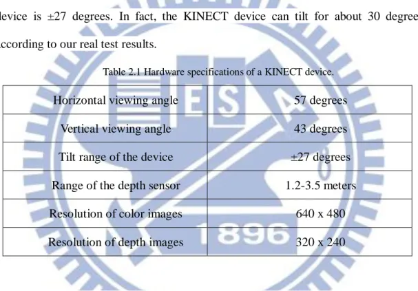
VGA video camera, a depth sensor, a multi-array microphone, and a motor for tilting the device. The hardware specifications of the KINECT device [6] are sorted and listed in Table 2.1. The appearance of the KIENCT device [7] is shown in Figure 2.2. In this section, some experiences obtained during using KINECT devices in this study are described. From Table 2.1, we can see that the range of the depth sensor is 1.2 to 3.5 meters. In fact its working range is larger, from 0.8 to about 6.0 meters. In addition, the accuracy of the depth image is millimeter. The tilt range of KINECT device is ±27 degrees. In fact, the KINECT device can tilt for about 30 degrees according to our real test results.
Table 2.1 Hardware specifications of a KINECT device.
Horizontal viewing angle 57 degrees Vertical viewing angle 43 degrees Tilt range of the device ±27 degrees Range of the depth sensor 1.2-3.5 meters Resolution of color images 640 x 480 Resolution of depth images 320 x 240
Next, the desktop computer used as the monitoring controller is introduced. The processor is an Inter Core i7-3770 Quad-core CPU with a Transcend DDR3 16G RAM; and the graphics card is of model Gigabyte GV-R7750C 2GI. We choose to use such a powerful processor and so big memory in order to use the processor to analyze lots of image data.
Furthermore, iron brackets are introduced, which were designed for holding the KINECT devices around the car, as shown in Figure 2.3. Three bases are affixed to each of the four sides of the car, and two bases are affixed onto the rear-view mirrors
10
of the car, one on each side, as shown in Figure 2.4.
Figure 2.2 Appearance of the KIENCT device.
(a) (b)
Figure 2.3 A base for the KINECT device (a)Without a KINECT device. (b) With a KINECT device.
(a) (b)
(c) (d)
Figure 2.4 Around-car bases (a) A front view. (b) A back view. (c) A lateral view. (d) A rear-view mirror.
11
2.2.2 Software Configuration
In the software configuration, we first introduce one of the SDKs of the KINECT device — OpenNI. OpenNI is the open source which enables the KINECT device to work on a computer and help us to acquire color and depth information captured from KINECT devices. Furthermore, it drives the motor in the KINECT device for the purpose of adjusting the angle of elevation.
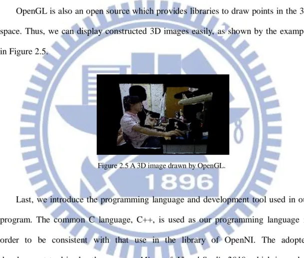
OpenGL is also an open source which provides libraries to draw points in the 3D space. Thus, we can display constructed 3D images easily, as shown by the example in Figure 2.5.
Figure 2.5 A 3D image drawn by OpenGL.
Last, we introduce the programming language and development tool used in our program. The common C language, C++, is used as our programming language in order to be consistent with that use in the library of OpenNI. The adopted development tool is also the common Microsoft Visual Studio 2010, which is used as the compiler of the program.
2.3 System Processes
2.3.1 Learning Process
12
images taken by neighboring KINECT devices, calibrating the relationship parameters of the devices are needed. Regarding the fact that a KINECT device is able to tilt in vertical direction, at the beginning of the calibration process, we use the libraries of OpenNI to adjust the device angle by controlling its motor to make sure its direction is parallel to the ground. Then, an ICP scheme is adopted for computing the horizontal angle and the displacement of the device with respect to its neighboring one.
Another task of learning is computing the environmental parameters. When driving on the road with different widths, setting different thresholds to filter out unrelated scenes is needed to obtain the monitoring target accurately. And we do this in our learning process as well. A flowchart of the proposed learning process is shown in Figure 2.6.
2.3.2 Monitoring Process
While driving on the road, once a ramp is discovered, the slope in degrees of the ramp will be displayed by the system as a warning to the driver. The system will also notify the driver a signal about whether to pass the ramp or not when driving to a place with a limitation on the car height, such as at the entrance of a parking lot, while going through a road under a bridge, etc. Furthermore, the driver is notified as well whether a car collusion is going to happen while encountering a by-passing car. Finally, after the car is parked, the system is used in an offline fashion to model around-car scenes, and analyze them to check the responsibility if legal cases about car accidents arise. A flowchart of the monitoring process is shown in Figure 2.7.
13
Start of
learning
filter threshold
OpenGL
3D
images
Remove
unrelated scene?
End of
learning
Yes
No
motor control
by OpenNI
ICP
Relationship
parameters
14 Start of Monitoring Driving? Around-car monitoring Ramp monitoring Height monitoring Collision monitoring Yes No
15
Chapter 3
Construction of 3D Images from
KINECT Images
3.1 Review of Pinhole Camera Model
The pinhole camera is a simple camera model with an aperture of only the pinhole size. It may be regarded as an opaque box with a pinhole on one side. The light passing the pinhole will produce an upside-down projection of the scene in front of the pinhole, as illustrated in Figure 3.1 [8].
Figure 3.1 An illustration of a pinhole camera model.
The pinhole camera model describes the mathematical relationship between a 3D point and its projection on the image plane of the pinhole camera. An illustration of the geometry of the pinhole camera model is shown in Figure 3.2. From the two similar triangles appearing in Figure 3.2(b), we can derive the following equation
16
according to the similar-triangle principle:
3 1 1 x x f y . (3.1)
When we look in the negative direction of the X1-axis, the following equation can
be derived similarly: 3 2 2 x x f y . (3.2)
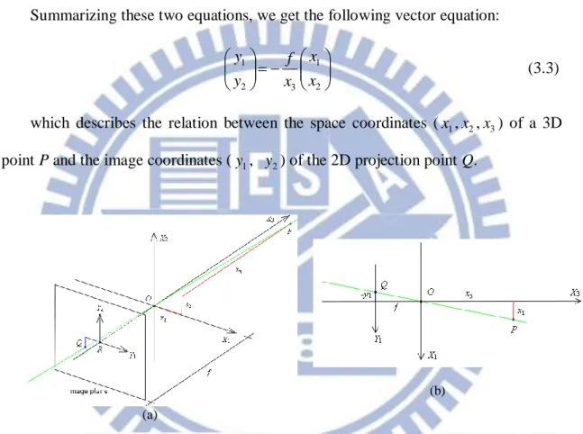
Summarizing these two equations, we get the following vector equation:
2 1 3 2 1 x x x f y y (3.3) which describes the relation between the space coordinates (x ,1 x ,2 x ) of a 3D 3 point P and the image coordinates (y , 1 y ) of the 2D projection point Q. 2
(a)
(b)
Figure 3.2 The geometry of a pinhole camera. (a) Seen from a 3D point. (b) Seen from the X1-axis.
3.2 Construction of 3D Images
3.2.1 Coordinate Conversion
17
And from Figure 3.2(a) and using the similar-triangle principle again, we have the equation:
where
2
2 2 1 2y y f
is the length of the line segment OQ, and 2 2 2 1 2 3
x x x
is the length of the line segment OP which is the depth captured by KINECT device, and is denoted as d in the sequel. Let R present the center of the depth image. It is located at coordinates (320, 240) in a depth image of resolution 640480 acquired by the KINECT device. And let Q be located at image coordinates (xp, yp)and let y1 and
y2 represent the distances to the center Q in the vertical and horizontal directions,
respectively. The letter f denotes the focal length of the KINECT device with its value being 600. The equations (3.7), (3.4), (3.5), and (3.6) can be rewritten, according to the mentioned parameter values, to be:
1 3 1 y f x x ; (3.4) 2 3 2 y f x x ; (3.5) f f x x 3 3 . (3.6)
2 2 2 2 1 2 3 2 2 2 1 3 f y y x x x f x (3.7)
2
2 2 3 600 240 320 p p y x d f x ; (3.8)
320
2 240
2 6002
320
1 p p p x y x d x ; (3.9)
320
2 240
2 6002
240
2 p p p y y x d x ; (3.10)18
The unit of xp and yp is pixel and that of x1, x2, and x3 is millimeter. With the
above equations, the coordinates in different coordinate systems can be converted successfully for 3D image construction as described next.
3.2.2 Idea of 3D Image Construction
The basic idea proposed in this study of 3D image construction is to convert the coordinates of the depth image described in Section 3.2.1 into 3D points. Then, we can draw these 3D points in the 3D space by the OpenGL. Finally, every RGB value of the pixel in the color image is “attached” to the corresponding 3D point. Colorful point clouds will be then formed in the resulting 3D image.
3.2.3 Construction Algorithm
In the proposed 3D image construction algorithm, assume first that the depth image coordinates are already converted into 3D points by coordinate conversion as described in Section 3.2.1. Then, it is desired to find the color information corresponding to each 3D point. By Equation (3.3) and the definitions given in Section 3.2.1, we have:
Therefore, the space coordinates (x1, x2, x3) of a 3D point can be used to find the
coordinates (xp, yp) of the corresponding image point. A flowchart of the resulting 3D
image construction algorithm is shown in Figure 3.3. A detailed description of the
600 600 240 3202 2 2 3 p p y x d x . (3.11)
3 1 600 320 x x xp or 600 320 3 1 x x xp ; (3.12)
3 2 600 240 x x yp or 600 240 3 2 x x yp . (3.13)19
algorithm is as follows.
Algorithm 3.1: 3D image construction.
Input: a depth image Id and a color image Ic captured by a KINECT device.
Output: a 3D image I3D formed from Id and Ic with colorful 3D points.
Steps:
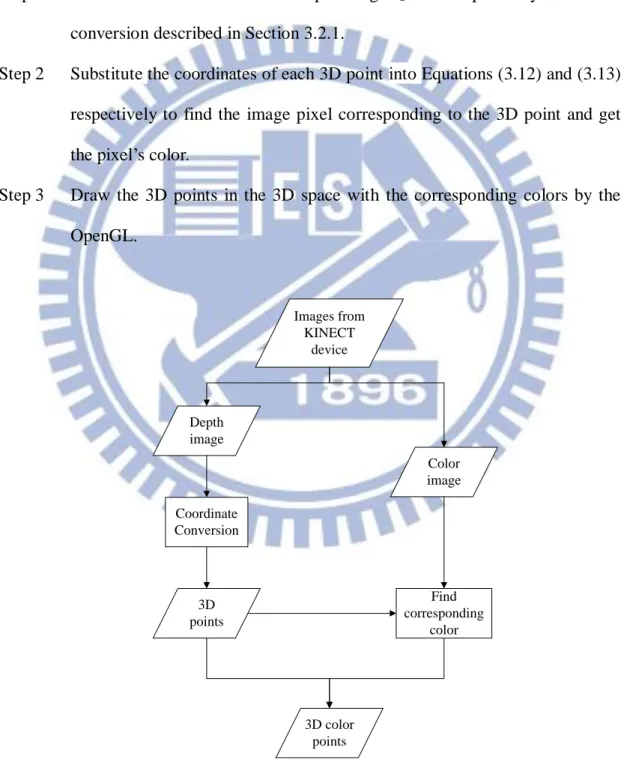
Step 1 Convert the coordinates of the depth image Id into 3D points by coordinate
conversion described in Section 3.2.1.
Step 2 Substitute the coordinates of each 3D point into Equations (3.12) and (3.13) respectively to find the image pixel corresponding to the 3D point and get the pixel’s color.
Step 3 Draw the 3D points in the 3D space with the corresponding colors by the OpenGL. Images from KINECT device Depth image Color image Coordinate Conversion Find corresponding color 3D points 3D color points
20
3.2.4 Experimental Results
Figure 3.4 shows the depth image and the color image which are the inputs to the algorithm of 3D image construction. After the algorithm is executed, we have the 3D images, as shown in Figure 3.5. To prove the output of the algorithm to be three-dimensional, Figure 3.5 (b) shows the top view of the 3D image from which the depth of the car in the 3D image can be seen obviously, confirming the 3D nature of the output of the algorithm.
(a) (b)
Figure 3.4 Images acquired by a KINECT device. (a) The depth image. (b) The color image.
(a) (b)
21
3.3 Review of a method for Geometric
Correction of 3D Images
3.3.1 Idea of Geometric Correction
From Figure 3.5 (b) in Section 3.2.4, we discovered that the farthest points of the depth image form an arc shape rather than a straight line. The reason why this problem arises is that the infrared light rays sent out by the KINECT device for depth sensing do not go in parallel as mentioned in Section.1.3. It affects the accuracy of the depth because the depth is not the vertical distance anymore. In order to solve the problem, a method for geometric correction of 3D images [9] is adopted.
The idea behind the proposed geometric correction method is that we use a paraboloid to approximate the curved surface formed by the farthest points of the depth image mentioned previously. Once the approximating paraboloid is found, the values of the coordinates x and y of each space point are substituted into the equation of the paraboloid to correct the computed distance, as shown in Figure 3.6.
22
3.3.2 Correction Algorithm and Experimental Results
In this section, the method for finding the approximating paraboloid is described and some experimental results are shown. The criterion of minimum sum of squared errors (MSSE) is used to decide the parameters of the approximating shape which is a paraboloid. The following is the detail of this process.
First, let the equation of the paraboloid be described by:
where C is the distance between the KINECT device and the apex of the paraboloid, as shown in Figure 3.6. The equation for computing the value SSE of the SSE is:
where (xi, yi, zi) are the coordinates of a sample point. To find the coefficients A, B and
C which minimize the SSE value, we compute the partial derivatives of Equation
(3.15) with respect to variables A, B and C, respectively, leading the following equations:
The values of A, B and C are computed by solving the simultaneous equations (3.16), (3.17) and (3.18). Since we have all the values of xi, yi and zi, the equations
(3.16), (3.17) and (3.18) become the three-variable linear equations after substituting all the values of xi, yi and zi into the simultaneous equations. By solving these three
independent equations, the values of A, B and C can be computed analytically. The
C y B x A zp 2 2 (3.14)
640480 0 2 2 2 i i i i i A x B y C z SSE (3.15)
0 2 2 480 640 0 2 2
i i i i i i A x B y C x z ; (3.16)
0 2 2 480 640 0 2 2
i i i i i i A x B y C y z ; (3.17)
1 0 2 480 640 0 2 2
i i i i i A x B y C z . (3.18)23
demanded paraboloid is so obtained. Finally, we show some examples of the experimental results in Figures 3.7 and 3.8.
(a) (b)
Figure 3.7 A correction result of Figure 3.5 (b). (a) Before correction. (b) After correction.
(a) (b)
24
Chapter 4
Modeling of Around-car Events
4.1 Construction of Around-car 3D
Images
In this chapter, we describe the method we propose for modeling of around-car events. In Section 4.1.1, the iterative closest point (ICP) algorithm and the K-D tree algorithm [10] used in this study are reviewed. In Section 4.1.2, how the calibration work is done by using the ICP algorithm to find the geometric relationship between every two KINECT devices is presented. With the calibration information, the idea and algorithm for constructing the around-car model are proposed in Sections 4.1.3 and 4.1.4, respectively. Finally, we show some experimental results in Section 4.1.5.
4.1.1 Review of Iterative Closest Point (ICP)
Algorithm and K-D Tree Algorithm
The iterative closest point (ICP) algorithm can be employed to minimize the difference between two groups of points. The concept of the algorithm is simple. It revises the transformation, including rotation and translation, from one object to the other, iteratively in order to minimize the total distance measure between the two groups of points.
The ICP is often used to match objects to compute their similarity. It is found useful for constructing 2D or 3D images from different views because object
25
registration or stitching, which is needed in this study, requires shape matching before the work is conducted.
A K-D tree algorithm is also employed in this study to reduce the amount of computation for searching the closest point using the ICP algorithm. The method for constructing a K-D tree, simply speaking, is to separate the group of points in concern into two parts by the median of the X, Y and Z coordinates sequentially. When searching the closest point, it takes less time to search a K-D tree rather than to search all the points. The complexity of searching becomes O(N2/3) from O(N).
4.1.2 Calibration between Neighboring KINECT
Devices Using ICP
In Section 4.1.1, it was mentioned that the ICP algorithm can be employed to minimize the difference between two groups of points. This inspired us to get the idea that we might use the ICP algorithm to “register” two objects if the two groups of points composing the objects are similar in their features. So, a method of calibration of the geometric relationship between two neighboring KINECT devices using the ICP algorithm is proposed in this study, and is described in this section.
First, a carton is put between every two neighboring KINECT devices as the calibration target. Then, depth images are acquired with these two KINECT devices, respectively. At this moment, we have two similar groups of points which come from an identical object, the carton, but appear in two different views. After the ICP algorithm is applied to register them, geometric relationship parameters, including the horizontal included angle and the displacements along the x-, y- and z-axes can be obtained. This completes the calibration of the geometric relationship between two neighboring KINECT devices. A detailed description of this process as an algorithm is
26
as follows.
Algorithm 4.1: calibration between two neighboring KINECT devices using the ICP algorithm.
Input: depth images I1 and I2 of a calibration target (a carton) acquired respectively
with two neighboring KINECT devices D1 and D2.
Output: the geometric relationship parameters, a horizontal included angle i and a
3D displacement di, of D1 and D2.
Steps:
Step 1 Convert the coordinates of the depth images I1 and I2 into two groups G1
and G2 of 3D points, respectively, by the coordinate conversion scheme
described in Section 3.2.1.
Step 2 Move group G1 of 3D points iteratively through a series of transformations
Ti, each including a horizontal included angle i and a 3D displacement di =
(dix, diy, diz) along the x-, y- and z-axes, respectively.
Step 3 For each transformation Ti = (i, di), compute the Euclidean distances Djk
from each point Pj of G1 to every point Pk of G2.
Step 4 For each point Pj, choose the minimum distance Djm from the distances Djk.
Step 5 Sum up all the Djm as the distance Di for Ti between G1 and G2.
Step 6 Find the transformation Ti = (i, di) with the minimum Di as the desired
relationship parameters.
4.1.3 Idea of Proposed Method for Around-car Scene
Model Construction
According to the discussions in Section 3.2, we can construct a 3D partial scene model by the use of a single KINECT device. To construct the around-car 3D scene
27
model, a technique to use of multiple KINECT devices simultaneously is needed. And the relationship information for every two KINECT devices, which is obtained during calibration as described previously, is also needed. Under these conditions, we can start to construct the around-car scene model.
4.1.4 Construction Algorithm
In Section 2.1, we discuss how to use a desktop computer to control multiple KINECT devices to work simultaneously via a USB expansion card. As for calibration, the proposed method for acquiring the geometric relationship parameters between neighboring KINECT devices has been described in Section 4.1.2. A flowchart of the proposed around-car model construction algorithm is shown in Figure 4.1. And a detailed description of the algorithm is as follows.
Algorithm 4.2: around-car scene model construction.
Input: images I1 through I14 acquired with the 14 around-car KINECT devices,
respectively.
Output: an around-car model Mcar.
Steps:
Step 1 Construct 3D models M1 through M14 using images I1 through I14,
respectively, by the 3D image construction scheme described in Section 3.2.3.
Step 2 For i = 1~13, compute the geometric relationship parameters Ri between the
3D models Mi and Mi+1 iteratively by the calibration algorithm (Algorithm
4.1) described in Section 4.1.2, with each Ri including a horizontal angle i
and a 3D displacement di = (dix, diy, diz) along the x-, y- and z-axes,
respectively.
28
3.1 Rotate the x- and z-axes of 3D model Mi+1 by horizontal angles 1
through i iteratively in order to match the coordinate system of 3D
model M1.
3.2 Move the coordinates of 3D model Mi+1 through a series of 3D
displacements, namely, d1, d2, …, di iteratively to form an around-car
model Mcar.
Step 4 Display an around-car model Mcar by drawing all the point sets P1 to P14 of
3D models M1 to M14, respectively, in the 3D space with the OpenGL.
Images from multiple KINECT devices Calibration process Relationship information 3D image construction 3D models Around-car model OpenGL
Figure 4.1 A flowchart of the around-car model construction algorithm.
4.1.5 Experimental Results
29
around-car scene model construction are shown. At first, the comparative illustrations from Section 4.1.2 are shown in Figure 4.2. From Figure 4.2(b), it can be seen that after calibration, the 3D models of the identical cartons constructed from images acquired with two neighboring KINECT devices overlap each other well. Then, the constructed around-car model is shown from each of the three sides of the car respectively, as shown in Figure 4.3.
(a) (b)
Figure 4.2 Comparison of constructed 3D scene models before and after calibration. (a) Before calibration. (b) After calibration.
(a)
(b) (c)
30
4.2 Modeling of a By-passing Car Using
3D Distance-weighted Correlation
(DWC)
4.2.1 Review of DWC
The measure of distance-weighted correlation (DWC) was proposed by Fan and Tsai [11] originally for automatic Chinese seal identification. The measure is defined as the minimum distance between two groups S and T of pixels of seal imprint images after the seal imprint images are overlapped. For each pixel p in S, a pixel in T with the minimum distance to p is searched for. If the result is a pixel p' within a limited circular area A with a pre-selected radius K, then a weight wpK = 1/(dp2 + 1) is defined
where dp is the distance from p to p'; otherwise, the weight wpK is defined to be zero.
That is, for each pixel p in S, a weight wpK is defined as follows:
where dp is the distance of p in S to the closest point p' in T. Note that K is a threshold
used to decide an effective distance; distances larger than this threshold is discarded. Finally, the DWC defined for the two groups of pixels, S and T, is defined as follows:
where the coefficient 1/2 is included to treat S and T symmetrically; and NS and NT are
the total numbers of pixels in S and T, respectively. It can be verified that 0CK 1 and CK = 1 if and only if S = T. The DWC, though defined originally for seal
1 1 2 p K p d w , if 0dp K, 0 K p w otherwise, (4.1)
t T K t T S s K s S K w N w N T S C 1 1 2 1 , , (4.2)31
identification, is a general measure for point-type object shape matching.
4.2.2 Proposed 3D DWC
An extension of the above-reviewed “2D” DWC measure is proposed in this study for the purpose of 3D scene model construction. However, the 2D DWC was used to decide whether the images of two object shapes are similar or not, while the proposed 3D DWC is used to compute the displacement of two similar objects in this study.
4.2.3 Idea of Modeling of a By-passing Car Using 3D
DWC
The depth range of the KINECT device is limited and the horizontal angle is only 57 degrees, so we cannot acquire the 3D information of the entire scene from a single image frame. Therefore, it is difficult to construct a complete model of a scene with only one KINECT device, or equivalently, with only a pair of color and depth images acquired with a single KINECT device. But we discovered that the models in any two sequential image frames acquired with two neighboring KINECT devices, when acquired with a high frame rate, are very similar. Since it is possible to overlap the two similar objects by the 3D DWC as mentioned previously, the 3D DWC can thus help us construct the model of a scene from different frames acquired with distinct KINECT devices. As the 3D information increases, it is possible to construct a more complete model of a scene.
4.2.4 Modeling Algorithm
32
already constructed by one KINECT device as described in Section 3.2. Then, by the use of the 3D DWC, we compute the displacement between the 3D models which are constructed from the images acquired with every two KINECT devices. By using all the resulting displacements, it is feasible to construct a more complete model of a scene. In this study, the mainly concerned object in the scene model is a by-passing car. A flowchart of the modeling algorithm is shown in Figure 4.4. A detailed description of the algorithm is as follows.
Algorithm 4.3: modeling of a by-passing car using 3D DWC.
Input: a series I of image pairs I1, I2, …, In acquired of a by-passing car Mcar with n
KINECT devices, with each image pair Ii including a color image Ici and a
depth image Idi.
Output: a 3D model of Mcar.
Steps:
Step 1 Assuming that the car is driven in a road lane, learn the threshold T ofthe width of the lane in the depth images beforehand in order to remove background image parts beyond the lane in the next step.
Step 2 Perform the following steps to filter out unrelated scene parts other than the car in each image pair Ij, respectively, by the thresholds T learned in Step. 1:
2.1 for each pixel p in the depth image Idj, if the depth value of p is larger
than T, then remove p from Idj;
2.2 for each pixel p' in the color image Icj, if the corresponding pixel p in Idj
is removed, then also remove p' from Icj.
Step 3 For each image pair Ij,construct a 3D model of the by-passing car Mj by the
3D image construction scheme described in Section 3.2.3.
Step 4 For j = 1 through n 1 (i.e., for every two neighboring car models), perform the following steps to construct a complete car model Mcar:
33
4.1 compute the 3D displacement dj = (djx, djy, djz) along the x-, y- and
z-axes, respectively, by matching the two partial car models Mj and Mj+1
by the use of the 3D DWC measure described previously.
4.2 overlap the two partial car models Mj and Mj+1 in accordance with the
computed 3D displacements dj to form a new model to replace the
original partial model Mj+1.
Step 5 Display the resulting car model Mcar of the last step by drawing all the
overlapped points of Mcar in the 3D space with the OpenGL.
A series of image pairs of a by-passing car 3D image construction 3D car models 3D DWC Displacement of matching OpenGL A model of by-passing car Learning process Threshold ofthe width of the lane Filter out background
34
4.2.5 Experimental Results
In this section, an example of the 3D models of the by-passing car resulting from executing Algorithm 4.3 described previously is shown in Figure 4.5. It is obvious that with more image frames, the constructed model of the by-passing car becomes more complete. Furthermore, from Figure 4.5(a) we can see only the middle part of the car, but from Figure 4.5(d) we can see its rear part. This experimental result shows the effectiveness of the use of the 3D DWC measure for 3D object modeling.
(a) (b)
(c) (d)
Figure 4.5 The models of a by-passing car constructed by overlapping different numbers of frames. (a) By one frame. (b) By five frames.(c) By ten frames. (d) By fifteen frames.
35
4.3 Restoration of Car-accident Scenes
4.3.1 Idea of Restoring Car-accident Scenes Using 3D
DWC
Since the depth range yielded by the KINECT device is limited, as described previously, once the distance between the KINECT device and the object is out of the range, it becomes impossible to acquire the depth information. In addition, when a car accident occurs, we need to construct the models of the involved cars in order to clarify the responsibility of the car accident by inspecting the relative geometric conditions of the constructed car models. But the distance between the cars in a car accident is usually smaller than the minimum value of the depth range. Nevertheless, from the Section 4.2, we know that it is possible to increase 3D information by overlapping the models in continuous frames. That is, we can construct a more complete model of the involved car in the car accident by overlapping the models in the previous frames. This means that we can use the 3D DWC measure to restore a car accident scene. More details are presented in the following.
4.3.2 Restoring Algorithm
First, the depth and color images of the involved cars which appear just before the car collision happens are needed. Then, the backgrounds and the depth information, which do not belong to the car, are filtered out to construct the car models more easily. Next, the displacement for overlapping the car models is computed by the use of the 3D DWC measure, as done previously. Once the models of the involved cars are overlapped accurately with the displacement, we can restore the car accident scene by constructing more complete models of the involved cars. A
36
flowchart of the restoration algorithm is shown in Figure 4.6. A detailed description of the algorithm is as follows.
Algorithm 4.4: restoring of a car-accident scene using 3D DWC.
Input: an image sequence I1 through In of an involved car (other than the one on
which the proposed system is installed) in a car-accident.
Output: a complete model Mcar of the involved car.
Steps:
Step 1 Pick out the image Ij of the involved car which appears just before the car
collision occurs by inspecting the image sequence I1 through In acquired of
the involved car.
Step 2 Construct 3D models M1 through Mj from images I1 through Ij by the 3D
image construction scheme described in Section 3.2.3.
Step 3 For k = 1, 2, …, j1, compute the 3D displacement dk = (dkx, dky, dkz) along
the x-, y- and z-axes, respectively by matching the car models Mk and Mk+1
by the use of the 3D DWC scheme mentioned in Section 4.2.2.
Step 4 For k = 1, 2, …, j1, overlap the car models Mk and Mk+1 in accordance with
the computed 3D displacements dk to form a more complete model of the
involved car Mcar.
Step 5 Display Mcar by drawing all the points in Mcar in the 3D space with the
OpenGL.
4.4 Experimental Results
Due to security concerns, a toy car was used to simulate car accidents in this experiment. Figure 4.7 shows the models of the car before the instant of collision in a simulated car accident in different frames, respectively. The green lines simulate the
37
range of our car on which the proposed system is installed. In Figure 4.7(d), we can see that part of the toy car passes through the area surrounded by the green lines. It means that the toy car collides with our car. By the constructed model, it is feasible to restore a car-accident scene and check the responsibility in law.
An image sequence of the involved car 3D image construction 3D car models 3D DWC Displacement of matching OpenGL a complete model of the involved car
Pick out the specific image
sequence
38
(a) (b)
(c) (d)
Figure 4.7 Models of an involved car before the instant of collision in different frames. (a) 60 frames before. (b) 40 frames before. (c) 20 frames before. (d) At instant of collision.
39
Chapter 5
Real-time Response to Around-Car
Dangerous Events
5.1 Monitoring of Ramps on Roads
5.1.1 Idea of Monitoring of Ramps on Roads
The slope of the ramp, especially that of a downhill one, is important information for a driver while driving on the road. The speed of the car will rise because of the gravity when driving on a downhill road. As the speed of the car goes up, it reduces the driver’s reaction time. That will be a potential danger to driving safety. In order to reduce the danger, we propose a method of using KINECT images and trigonometric functions and mathematical geometry to measure the slope of the ramp. In this way, the driver can know the slope of the ramp before driving downhill. If the driver is able to slow down earlier on a steep downhill road, the driving safety is improved.
5.1.2 Monitoring Algorithm and Experimental
Results
In the proposed method, the KINECT device we use is mainly the one affixed in the front of the car, which is tilted down thirty degrees in order to increase the acquired depth information of the road, as shown in Figure 5.1. As seen in Figure 5.2, let θ3 represent the slope of the ramp. Then, it can be easily figured out from
40
trigonometry that
where θ1 is 30o as mentioned previously, and according to trigonometry again, we
have:
where ΔY and ΔZ can be computed by points P(Y1, Z1) and Q(Y2, Z2) which are
selected from the centerline of the KINECT device on the ramp. By Equation 5.1, the slope of the ramp θ3 can be computed. A flowchart of the algorithm is shown in
Figure 5.3. A detailed description of the algorithm for this process is as follows.
Algorithm 5.1: computing the slope of a ramp.
Input: a depth image I acquired with the KINECT device affixed in the front of the
car.
Output: a slope of a ramp. Steps:
Step 1 Select the lowest pixel point P on the image boundary from the centerline of the depth image I.
Step 2 Select the center point Q of the depth image I.
Step 3 Convert the coordinates and the depth values of pixel points P and Q into 3D points P(X1, Y1, Z1) and Q(X2, Y2, Z2), respectively, by the coordinate
conversion scheme described in Section 3.2.1.
Step 4 Compute ΔY and ΔZ by subtracting the values of Y1 and Z1 of point P from
the values of Y2 and Z2 of point Q, respectively, i.e., compute Y = Y1 Y2
and Z = Z1 Z2.
Step 5 Compute the angle θ2 by Equation 5.2.
θ3 = θ1 – θ2 (5.1) ) ( tan 1 2 Z Y (5.2)
41
Step 6 Compute as output the slope of the ramp θ3 by Equation 5.1.
Figure 5.1 The KINECT device affixed in the front of the car and it is tilted down thirty degrees.
42 x and z coordinates of points P and Q Trigonometric functions The degree of θ2 Alternate interior angles The slope of the ramp
Figure 5.3 A flowchart of computing slopes algorithm.
Once the slope of the ramp θ3 is computed, it is feasible to compute the
magnitude of gravity g, as shown in Figure 5.4. From the figure, we have:
where a represents the acceleration of the car along the ramp. Some results of computations of the value a in different slopes are shown in Table 5.1. Assume that the ramp is 100m long and the car speed is 40 km/hr. It takes 9 seconds to pass the ramp without the acceleration a. Once we have the acceleration, the time is shorter than 9 seconds. By the constant acceleration equation, we have:
where t denotes the passing time, s is the car speed, and l is the length the car goes. By
a = gcos(90o – θ3) (5.3)
2
1 2
43
substituting the acceleration a = 17.64 km/hr, the car speed s = 40 km/hr, and the slope length l = 100m into Equation (5.4), we can get the solution, the passing time, to be about 4.5 seconds which is a half of 9 seconds. It means that if the slope of the ramp is more than 30 degrees, the time will be less than a half of the time required for normal driving on flat road surfaces. Therefore, the driver should slow down the car speed to avoid danger.
Figure 5.4 The components of gravity g.
Table 5.1 The results of computations in different slopes.
Slope θ3 10o 20o 30o 40o 50o 60o
Acceleration a 6.12 12.06 17.64 22.68 27.03 30.55 km/hr
We now show some experimental results of applying the above algorithm to real situations. Figures 5.5 and 5.6 show two different results on the ground and on a ramp, respectively. Figures 5.5(a) and 5.6(a) show respective images of the ground and the
44
ramp in front of the car while Figures 5.5(b) and 5.6(b) respectively show the slopes of the ground and the ramp, respectively. The repeated values in Figures 5.5(b) and 5.6(b) denote keep monitoring the ramp.
(a)
(b)
Figure 5.5 The experimental result on the ground. (a) Front view from the car. (b) The values of the slope.
(a)
(b)
Figure 5.6 The experimental result on the ramp. (a) Front view from the car. (b) The values of the slope.
45
5.2 Monitoring of Limitations of
Heights on Roads
5.2.1 Idea of Monitoring of Limitations of Heights on
Roads
When driving on the road, there are some places where limitations on the car height are imposed, such as at the entrance of a parking lot, while going through a road under a bridge, etc. Despite of the fact that normally, there is a height limit sign which is used to warn the driver of hitting the car roof, the driver generally does not know the actual height of their car. Once the driver misjudges the height of the car, an accident of hitting the car roof might happen. To avoid such an accident, we use the KINECT device which is affixed on the front top of the car to monitor the height-restricting barriers and calculate the height difference between them.
5.2.2 Monitoring Algorithm and Experimental
Results
As mentioned previously, the KINECT device affixed on the front top of the car as shown in Figure 5.7 is used to monitor height-restricting barriers and calculate the height difference between the car roof and the barriers. Now, we describe the proposed method to do so. From Figure 5.8, we see that y1 of point P denotes the
height of the car roof and y2 of the point Q denotes the lowest height of the
height-restricting barrier. Let Δy be the height difference between the points P and Q. We search for the point Q from the point P along the continuous depth points in the negative direction of the y-axis. The endpoint of the continuous depth points is the