雙選擇性通道下正交分頻多工系統中使用馬可夫鏈蒙地卡羅法之基於期望值最大化接收機設計

(1)

國

立

交

通大

學

電

信

工

程

學

系

碩

士

論

文

雙選擇性通道下正交分頻多工系統中使用

馬可夫鏈蒙地卡羅法之基於期望值最大化

接收機設計

Design of an EM-based Receiver Using the Markov

Chain Monte Carlo Method for OFDM Systems in

Doubly Selective Channels

研究生：鍾曉顗

指導教授：黃家齊博士

(2)

雙選擇性通道下正交分頻多工系統中使用馬可夫鏈

蒙地卡羅法之基於期望值最大化接收機設計

Design of an EM-based Receiver Using Markov Chain Monte

Carlo Method for OFDM Systems in Doubly Selective Channels

研究生：鍾曉顗 Student：Siao-Yi Jhong

指導教授：黃家齊 Advisor：Dr. Chia-Chi Huang

國立交通大學

電信工程學系碩士班

碩士論文

A Thesis

Submitted to Department of Communication Engineering College of Electrical Engineering and Computer Engineering

National Chiao Tung University in Partial Fulfillment of the Requirements

for the Degree of Master of Science

in

Communication Engineering June 2009

Hsinchu, Taiwan, Republic of China

(3)

雙選擇性通道下正交分頻多工系統中使用馬可夫鏈

蒙地卡羅法之基於期望值最大化接收機設計

學生：鍾曉顗指導教授：黃家齊博士

國立交通大學電信工程學系碩士班

摘要

雙選擇性(衰減)通道造成載波間干擾(Inter-carrier Interference, ICI)的問

題並降低系統效能，受到鄰近子載波之能量擴散而產生的載波間干擾效

應，是本論文首要的估測目標，因而提出一種正交分頻多工(Orthogonal

Frequency Division Multiplexing, OFDM)系統接收機，其為基於期望值最大

化演算法(Expectation-Maximization, EM)設計而成。在頻域模式下進行系統

分析，將 EM 演算法與馬可夫鏈蒙地卡羅法(Markov chain Monte Carlo,

MCMC)結合，並以最大相似度(Maximum Likelihood, ML)作為判定準則，

我們得到一套有系統地估測載波間干擾的方法，稱之為「EM 通道估測法」

。

此外，為了減低運算複雜度，以及充分利用時變通道所賦予的時間多樣性，

ML-EM 接收機採用「分群式載波間干擾消除器」

，針對通過此消除器之後

的接收信號，估算適當的殘餘載波間干擾功率，以提高資料偵測的正確率。

電腦模擬結果顯示，相較於以往一階等化器，我們提出的 ML-EM 接收機在

錯誤率方面的表現，有著明顯的進步。

(4)

Design of an EM-based Receiver Using Markov Chain

Monte Carlo Method for OFDM Systems in Doubly

Selective Channels

Student：Siao-Yi Jhong

Advisor：Dr. Chia-Chi Huang

Department of Communication Engineering

National Chiao Tung University

ABSTRACT

Doubly selective (fading) channels cause the inter-carrier interference (ICI) problem and thus degrade the system performance. In order to estimate the ICI effect made by the spreading energy of adjacent subcarriers, we propose an expectation-maximization (EM)-based receiver for orthogonal frequency division multiplexing (OFDM) systems. In this paper, we use the frequency domain model for system analysis and derive the EM channel estimation method by combining the Markov Chain Monte Carlo (MCMC) method with the EM algorithm according to the maximum-likelihood (ML) criterion. Besides, the proposed EM-based receiver is incorporated with the group-wise ICI cancellation method for reducing computational complexity and exploiting the inherent time diversity in time-variant channels. After the ICI cancellation, the residual ICI power is calculated for the ICI-reduced signals with the goal of making data detection more correctly. Results of computer simulation demonstrate that the ML-EM receiver performs much better than the conventional one-tap equalizer.

(5)

誌謝

這一年來，投入研究的時間佔據了我大部分的生活，而研究過程的起

伏帶來喜怒哀樂各種情緒，留下一段非常難忘的經驗。雖然現在的我，還

是有很多事情弄不明白，但是跟一年之前的我相比，我想應該有了一點進

步。由於許多人的幫忙與鼓勵，使我能夠順利完成畢業論文。首先，我要

感謝黃家齊老師，與他談話有種如沐春風的愉悅，謝謝老師一直以來的關

心與指導。另外，感謝實驗室學長姊的提攜，特別是古孟霖學長與陳文娟

學姊，總是不厭其煩地教導、鼓勵我，為迷途的我指點前進的方向。接著，

我想感謝實驗室同學，這四位男生有著截然不同的個性，卻都很平易近人，

謝謝他們陪伴我度過研究所的時光。最後，感謝家人和朋友，包容我的任

性、體諒我的慌張、接納我的執著，因為他們，使我更有勇氣。

(6)

中文摘要 ….….……….………... i

ABSTRACT ….……….……….. ii

誌謝 ...……….……… iii

Contents ....………...……….. iv

List of Figures ….………... vi

Chapter 1 Introduction ..………..…... 1

Chapter 2 OFDM System Model ………...……... 5

2.1 Frame Format ………...……….……..…...

5

2.2 Doubly Selective Channels

………….……….

5

2.3 Transmitted Signals and Received Signals ….………...…

8

2.4 The ICI Model ……….……

10

Chapter 3 Gibbs Sampling ……….... 14

Chapter 4 The ML-EM Receiver ………. 16

4.1 Channel Estimation ………..…………...

16

4.1.1 E-step and M-step ..……….………..… 17

4.1.2 Derivation of Estimated Channel Slopes …..……….… 20

4.2 Data Detection by Gibbs sampling ….……...…….……….…

22

4.3 Initial Setting ……….……….……...……….

25

4.4 EM-based Channel Estimation Method ……….…….……….……

27

4.5 Group-wise Method ……….…....…..…..

28

Chapter 5 ICI Power Calculation ………. 32

(7)

6.1 System Parameter ………….………….……....………... 37

6.2 Simulation Results ……….……... 38

Chapter 7 Conclusions ……….. 55

(8)

List of Figures

Fig. 2.1 The allocation of subcarriers in OFDM systems…………..……….…………. 5

Fig. 2.2 An illustration of the equivalent impulse response……….… 7

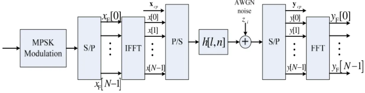
Fig. 2.3 OFDM Systems……….………. 8

Fig. 4.1 Initialization for ML-EM receivers………... 26

Fig. 4.2 An illustration of group-wise detection……….………...… 28

Fig. 4.3 The ML-EM receiver for OFDM systems………...… 31

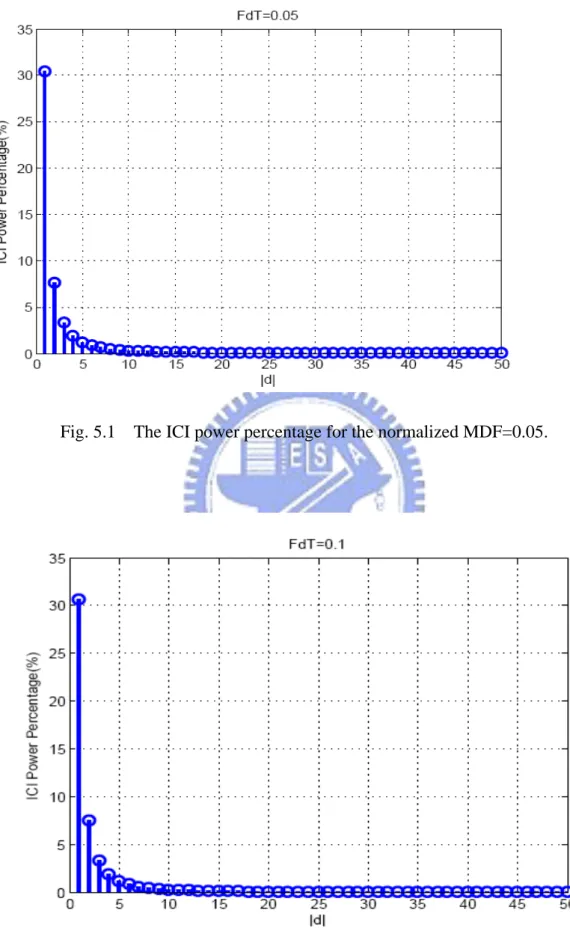
Fig. 5.1 The ICI power percentage for the normalized MDF=0.05 ...………..………... 36

Fig. 5.2 The ICI power percentage for the normalized MDF=0.1 ….…………..………...….. 36

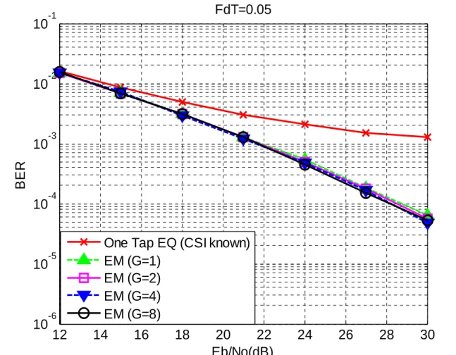
Fig. 6.1 BER performance of the ML-EM receiver with different group sizes for the normalized MDF=0.05 ………..……….………...… 41

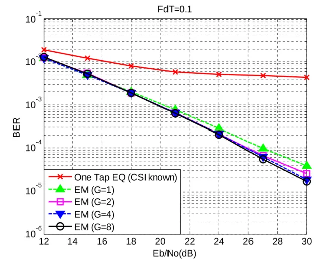
Fig. 6.2 BER performance of the ML-EM receiver with different group sizes for the normalized MDF=0.1 ………...………….………... 42

Fig. 6.3 BER performance of the ML-EM receiver with/w.o. ICI power update for the normalized MDF=0.05 ………..………... 43

Fig. 6.4 BER performance of the ML-EM receiver with/w.o. ICI power update for the normalized MDF=0.1 ………..………..………... 44

Fig.6.5 BER performance of the ML-EM receiver for the normalized MDF=0.05………... 45

Fig.6.6 BER performance of the ML-EM receiver for the normalized MDF=0.1………...…. 46

Fig.6.7 BER performance of the ML-EM receiver with/w.o. CE refinement for the normalized MDF=0.05 ……….……… 47

Fig.6.8 BER performance of the ML-EM receiver with/w.o. CE refinement for the normalized MDF=0.1 ……….………….……..………... 48

Fig.6.9 BER performance of the ML-EM receiver with different cases in the ITU Veh-A channel for the normalized MDF=0.05……..………...…… 49

(9)

Fig.6.10 BER performance of the ML-EM receiver with different cases in the ITU Veh-A channel for the normalized MDF=0.1……….……… 50 Fig.6.12 BER performance of the ML-EM receiver in different cases for the

normalized MDF=0.05……….……...…. 51 Fig.6.12 BER performance of the ML-EM receiver in different cases for the

normalized MDF=0.1 ……….…...……. 52 Fig.6.13 BER performance of the ML-EM receiver with various numbers of samples

for the normalized MDF=0.05 ……….... 53 Fig.6.14 BER performance of the ML-EM receiver with various numbers of samples

(10)

Chapter 1 Introduction

Over the last few years, the mobile communication technology develops rapidly, and

so do the wireless techniques. The wideband transmission became an inevitable trend because of the data rate demanded by users. The wireless network has the advantage of the mobility, the convenience and the high-coverage. Limits of time and place do not restrain the

communication among people. However, the channel of the wireless communication is interfered with by severe noise, and the multipath effect is also a problem which should be overcome. The multipath propagation causes the frequency selective fading and the

inter-symbol interference (ISI), and thus harms the quality of transmission and degrades the system performance. It would be significant to choose an appropriate system model according to the channel conditions and the requirements for transmission.

There are many techniques invented for raising the utility rate and mitigating the influence of the multipath effect, and orthogonal frequency division multiplexing (OFDM) is one of the most famous schemes. In OFDM, subcarrier frequencies are chosen to be

orthogonal to each other; namely, the crosstalk between the sub-channels is eliminated. The orthogonality also provides high spectral efficiency since almost the whole available

frequency band can be utilized. The duration of each symbol is long enough to put in a guard interval to eliminate the ISI, and the cyclic prefix (CP) used as the guard interval consists of a copy of the end of the OFDM symbol. Besides, OFDM is equipped for coping with

(11)

attenuation of high frequencies in a long copper wire and narrowband interference. The effect of frequency selective fading can be considered as flat over an OFDM sub-channel if its band is sufficiently narrow. This makes the equalizer simpler at the receiver compared with

conventional single-carrier modulation.

OFDM requires accurate frequency synchronization between the receiver and the transmitter. The subcarriers are no longer orthogonal if there is frequency deviation, inducing the inter-carrier interference (ICI). Frequency offsets are typically caused by mismatched transmitter and receiver oscillators, or by Doppler shift due to movement, and this effect worsens as speed increases or as the length of a symbol gets longer. In communication systems, the transmission often proceeds in the high- mobility condition, but the time-variant channels damage the orthogonality, cause the ICI effect and then lower the system

performance. As a result, the ICI suppression is a significant issue for research in mobile communication, and it is also the main study in this paper.

There have been many techniques suggested for the ICI suppression; for example, minimum mean square error (MMSE) [3], minimum mean square error with successive detection (MMSE-SD) [3], polynomial cancellation coding (PCC) [4] and self-cancellation coding [5]. The method in [3] is efficient but with high computational complexity. The schemes in [4] and [5] provide good bit error rate (BER) performance at the expense of sacrificing bandwidth efficiency. In [6] and [7], the piece-wise linear model is proposed to

(12)

approximate the channel variation, helping the analysis of properties of the channel. It is explained that energy of a sub-carrier leaks to the adjacent sub-carriers owing to Doppler shift in [8] and [9]. The expectation-maximization (EM) algorithm can be utilized to solve the maximum-likelihood (ML) estimation problem in an iterative manner. Recently, some EM-based methods have been proposed for channel estimation and data detection in OFDM systems. But the wireless channel is assumed to be quasi-static, i.e., channel gain remains constant over the duration of one OFDM symbol.

In this paper, we propose an EM-based receiver for OFDM systems in doubly selective fading channels. By assuming channel varies in a linear fashion, we analyze the ICI effect in frequency domain and derive a channel estimation method based on the EM algorithm in [10] and [11] under the ML criterion. A Gibbs sampler (a Markov chain Monte Carlo procedure) is used for the calculation of Bayesian estimates and also for data detection in the EM algorithm. Moreover, we combine the EM-based receiver with a group-wise ICI cancellation scheme for the sake of reducing the computational complexity. The ML-EM receiver is implemented to iterate between a group-wise ICI canceller and an EM detector (including the Gibbs samplers inside). The MMSE estimator is employed in the receiver for the initial setting by exploiting the pilot tones in each frame, and the accuracy of initialization can be refined successfully through the mechanism of decision feedback.

(13)

described and the ICI effect is analyzed in frequency domain. And the basic idea of the Gibbs sampling method is briefly introduced in Chapter 3. In Chapter 4, a channel estimation method is derived from the EM algorithm combined with a Gibbs sampler using the ML criterion, and accordingly, we propose an ML-EM receiver for OFDM systems. And the ML-EM receiver is further united with the group-wise method in chapter 4.The problem of computing the ICI power (or the variance of ICI) for the Gibbs sampling is treated in Chapter 5. Results of computer simulation are presented and discussed in Chapter 6. In the final part of the paper, Chapter 7, we draw some conclusions for the study.

The following are some interpretations of notations used in the paper. Boldface capital letters denote matrices, whereas boldface lowercase letters denote column vectors. The superscripts and stand for the transpose and the Hermitian transpose of a matrix, respectively. The column vector can be explicitly expressed by

( )

T ⋅

( )

H ⋅ x x x₁, ₂,…,x_x or

{

}

:

1,

,

i

x i

∈

…

x

, where x is the dimension of the vector x. The notation

{ }

…

represents a set, e.g. a set x=

{

x ,₁…, x_x

}

, and the cardinality of the set x is denoted by x . The set can also be expressed in a compact form:

{

x i_i : ∈

{

1,…, x

}

.

(14)

Chapter 2 OFDM System Model

2.1 Frame Format

According to the frame format in IEEE 802.16e standard [12], a frame consists of the pilot preamble in the first symbol followed by many OFDM symbols carried by numerous subcarriers. The number of subcarriers depends on the size of the Fast Fourier Transform (FFT), and there are three types of subcarriers shown in Fig. 2.2. First, the data subcarriers are used to transmit data symbols. And the pilot subcarriers are used as virtual subcarriers to help the channel estimation. In an OFDM symbol, a sequence of values is inserted to be the pilot signals. Moreover, the null subcarriers can be the DC subcarriers or the guard band which alleviates the aliasing problem at the receiver.

Fig. 2.1 The allocation of subcarriers in OFDM systems.

2.2 Doubly Selective Channels

(15)

high capacities that result in doubly selective channels. Doubly selective fading means frequency selective fading induced by the multipath propagation and time selective fading caused by the time-varying channel.

The multipath propagation is a phenomenon that the transmitted signals arrive at different times at the receiver through more than one path. The time difference between the arrival moment of the first multipath component and the last one is called delay spread. The coherence bandwidth measures the separation in frequency which two signals experience uncorrelated fading. If the coherence bandwidth of the channel is smaller than the bandwidth of the signal, different frequency components of the signal suffer from decorrelated fading. The channel varies with time due to Doppler shift resulted from rapid traversing of the transmitter or the receiver. The coherence time is a measure of the minimum time required for the magnitude change of the channel to become decorrelated from its previous value. When the coherence time of the channel is small relative to the symbol duration, the amplitude and phase of the signal change imposed by the channel varies considerably, causing a fast fading channel.

That is, the doubly selective channel is also called the frequency-selective fast-fading channel. The equivalent impulse response can be expressed as follows:

( )

(

( ) 1 , L l l l h t τ α t δ τ τ

)

= =

∑

− (2.1) where αl

( )

t and ( )l

(16)

and δ

( )

⋅ is the Kronecker delta function. The complex fading gain is a function of which denotes the time index, and the value stands for the number of paths. Fig. 2.2 below is intended to show the equivalent impulse response.

t

L

( )

t

The variation of the fading gain,αl , which depends upon Doppler shift is proportional to the carrier frequency and the speed of a motor vehicle. The maximum Doppler frequency (MDF) is defined as _D c c f v f = (2.2) where v is the velocity of the source relative to the receiver, f is the carrier frequency and c

is the speed of light (e.g. 3×108 m/s for light travelling in a vacuum). In OFDM systems, the normalized MDF

c

D s

f T (in which T is the sampling period) is used to indicate the range s

of variation in the channel. By keeping T and s f constant, it can be observed from (2.2) c that f becomes larger when the car is driven faster. D

t

( )

, h t

τ

2

τ

4 0 t 1 t 2 t 3 t 1

( )

t3

τ

( )

t2

τ

( )

t1

τ

( )

t0

τ

3

τ

_N₋₂

τ

_N₋₁

τ

0

τ

Fig. 2.2 An illustration of the equivalent impulse response.

(17)

2.3 Transmitted Signals and Received Signals

[0] x [1] x [ 1] x N− cp x

[ , ]

h l n

[0] y [1] y [ 1] y N− cp y F[0] y

[

]

F 1 y N− i z F[0] x

[ ]

F 1 x N−

Fig. 2.3 OFDM Systems.

Fig.2.3 shows an OFDM system. The information source bits are mapped into MPSK data symbols and are converted into N parallel data streams through a serial to parallel (S/P) block. Then the data streams are modulated onto N subcarriers by an N-point inverse Fast Fourier Transform (IFFT) unit to produce samples in the time domain, and the transmitted signal is expressed as 2 1 0 1 [ ] [ ] mn N _j N m x n X m e N π − = =

∑

(2.3) where X m

[ ]

represents the data in frequency domain at the th subcarrier. For the

purpose of eliminating ISI due to multipath channels, a CP is added at the head of each data symbol, being presented as

m

x nc

[ ] [

=x N+n

]

, n= −NG,…, 1− (2.4) where is the length of the guard interval. We assume that the maximum delay spread of the channel is always smaller than to make sure that there is no ISI after removing the guard interval.

G N

(18)

received OFDM symbols in time domain can be expressed as the circular convolution of the transmitted symbols and the channel impulse response; hence, received signals are given by

(2.5) 1 [ ] [ ] [ , ] [ ] [ , ] [(( )) ] [ ] L N l y n x n h l n z n h l n x n l z n = = ⊗ + =

∑

− +

where represents the channel impulse response of the th channel tap at the th sample time, is the delay time of the th path relative to the first path, is the discrete time index, [ , ] h l n

[

l n l l n

]

z n 2 z

is a sample of additive white Gaussian noise (AWGN) with zero-mean and variance σ , and (( ))i _N means a cyclic shift in the base of N.

After removing the guard interval and taking the Fast Fourier Transform (FFT), the received signals in frequency domain can be described by

(2.6)

[ ]

[

] [ ]

[ ]

[ ] [ ]

[

] [ ]

[ ]

1 F F F 0 1 F F 0, ICI term , , , N m N m m k y k H k m x m z k H k k x k H k m x m z k − = − = ≠ = + = + +

∑

F

in which x kF

[ ]

is the transmitted signals in frequency domain and H k k

[ ]

, is the

frequency response of the average gain of the channel. And H k m

[

,

]

, which represents the leakage factor of ICI from the th subcarrier to the th subcarrier, is provided in the following: m k

[

]

[

]

2 1 0 , , , ml L _j N l H k m k m l e π β − ₋ = =

∑

(2.7) where β[ , , ]k m l is the frequency response of the time-varying channel and can be given by

2 (( )) 1 0 1 [ , , ] [ , ] N n k m N _j N n k m l h l n e N π β − − − = =

∑

. (2.8)

(19)

Accordingly, H k m

[

,

]

is regarded as the summation of α[ , , ]k m l multiplied by the linear phase resulted from the time delay of the th tap. l

If the channel is time-invariant in the OFDM symbol duration; namely, it is in the slow fading mode,H k m

[

,

]

turns out to be zero when k and m are different values, and thus

[

,

]

H k m is equivalent toH k k

[ ]

, . That is, there is no ICI among subcarriers.

2.4 The ICI Model

In [6] and [7], with the normalized MDF up to 0.1, a first-order polynomial function is adequate to model the time variation of each channel tap in an OFDM symbol and it

is defined by

h l n[ , ]=a[ ,1]l n+a[ , 0]l (2.9)

where a l p[ , ] is the coefficient of p th monomial in the function of the th path. By substituting (2.9) to (2.8),

l

[ , ,k m l]

β can be presented as follows:

(i)m=k:

[

, ,

]

1

[ ] [

,1 , 0 2 N k m l a l a l β = − +

]

(2.10) (ii)m≠k: β

[

k m l, ,

]

= Φ

[

k m a l,

] [ ]

,1 (2.11) where

[

]

( )

(

)

(

)

2 1 0 1 1 1 , 2 2 tan n k m N _j N n N k m ne j N k m N π π − − ₋ = Φ = = − + ⎛ − ⎞ ⎜ ⎟ ⎜ ⎟ ⎝ ⎠

∑

. (2.12)

And the Malcaurin series can be used to replace the tangent function in (2.12). A parameter λ is in the interval between

2

π

− and 2

π

(20)

in one variable expressed as follows:

tan 1 3 2 5 ... 3 15

λ = λ+ λ + λ + (2.13)

in which the high-order terms, i.e. λ3, λ5, may be neglected as the value of λ is smaller than one, and thus (2.13) can be written as

tanλ λ≈ . (2.14) The values of m and are within the range from 0 to k N−1, so

(

)

N

k−m is between 0

and N−1, and then

(

k m

)

N N π − in (2.12) is in the interval of , (N N N π π −1) ⎡ ⎤ ⎢ ⎥ ⎣ ⎦ or

(

0,π

)

.

(

)

(

)

tan k m N N ⎛ − ⎞ ⎜ ⎜ ⎝ ⎠ π ⎟

⎟ is simplified by the Malcaurin series, and so is Φ

[

k m,

]

which can be

classified in the following cases:

(i) (( )) tan (( )) tan

2 2 N N k m k m N N π − ₌π _⇒ ⎛π − ⎞₌ ⎛π ⎜ ⎜ ⎟ _{⎝ ⎠} ⎝ ⎠ ⎞ ⎟ , but tan 2 π ⎛ ⎞ ⎜ ⎟ ⎝ ⎠ is infinite, and therefore

[

,

]

1 2 k m Φ = − . (ii) 0 (( )) 2 N k m N π − π < < , so

[

]

(

)

(

)

1 , 2 2 N N k m j k m π Φ = − + − .

(iii) Subtracting π from (( )) 2 N k m N π π − _π

< < , we can get a new inequality of

(

)

(

)

0 2 N k m N N π π ⎡_⎣ − − ⎤

− < ⎦ < which conforms to the range required by the

Malcaurin series, and thus

[

]

(

)

(

)

1 , 2 2 N N k m j k m N π Φ = − + ⎡ ₋ ₋ ⎤ ⎣ ⎦ .

When k is different from m, Φ

[

k m,

]

can be formed in accordance with the results of (i), (ii) and (iii), and given by

(21)

1 for 0 (( )) 2 2 (( )) 2 1 [ , ] for (( )) 2 2 1 for (( )) 2 2 [(( )) ] 2 N N N N N N N j k k m N k m k m N N m j k m N k m N π π ⎧ − + < − < ⎪ ₋ ⎪ ⎪ Φ ≈_⎨ − − = ⎪ ⎪− + < − < ⎪ ₋ ₋ ⎩ . (2.15)

As a result, (2.12) can be replaced by the approximation in (2.15).

By making use of (2.11) and (2.15), the equation in (2.6) is rewritten as

1 F F F 0 [ ] [ , ] [ ] [ , ] [ ] [ ] [ ] N m m k F y k H k k x k k m w m x m z k − = ≠ = +

∑

Φ + (2.16) where

[ ]

2 1 0 ,1 ml L _j N l w m a l e π − ₋ =

=

∑

is defined as the channel variable in frequency domain and

[

k m,

]

Φ represents a fixed-valued coefficient of the ICI term. In order to provide a more

compact representation, we rewrite (2.16) in a matrix form which is given by

y Hx z= + =(M + ΦW x z Mx + ΦXw z ) + = + (2.17) where the

(

k m,

)

th entry of H is H k m

[

,

]

, y=_⎣⎡y_F

[ ]

0 ,…,y_F

[

N−1

]

⎤_⎦T,

[ ]

[

{

]

T

}

F , F diag x N = − X ⎡_⎣x 0 ,… 1⎤_{⎦ ,} x=⎣⎡xF

[ ]

0 ,…,xF

[

N−1

]

⎤⎦T,

[ ]

[

]

T F 0 , , F 1 z z N ⎡ ⎤ =_⎣ − _⎦ z … , M=diag

{

_⎣⎡H

[ ]

0, 0 ,…,H N

[

−1,N−1

]

⎤_⎦T

}

,

[ ]

[

]

{

T

}

0 , , 1 diag ⎡w w N ⎤ = _⎣ − _⎦ W … , w=⎡_⎣w

[ ]

0 ,…,w N

[

−1

]

⎤_⎦T and Φ is an matrix expressed in (2.18) below in which

N×N

[

k m,

]

Φ represents the

(

k m,

)

th entry. Furthermore, where

=

w Fa = ⎣⎡a

[ ]

0,1 , ,a

[

L−1,1

]

⎤_⎦T L

a is a vector composed of slopes of channel paths and is a DFT matrix of size

…

F N× with the

( )

m l, th entry provided by 2 [ , ] exp ml F m l j N π ⎧ ⎫ = _⎨− _⎬ ⎩ ⎭.

(22)

0 1 1 1 2 1 0 1 1 2 1 1 1 0 2 2 1 1 1 1 0 2 N N j j N N j j N N j j N j N N N j j j π π N j N j π π π π π π π π π π ⎡ ⎛ ⎞ ⎛ ⎞ ⎛ ⎤ − + − + − − ⎢ ⎜ ⎟ ⎜ ⎟ ⎜ ⎥ ⎝ ⎠ ⎝ ⎠ ⎝ ⎢ ⎥ ⎢_⎛ _⎞ _⎛ _⎞ _⎛ ⎥ ⎢_⎜− − _⎟ _⎜− + _⎟ _⎜− − ⎥ ⎢⎝ ⎠ ⎝ ⎠ ⎝ ⎥ ⎢ ⎥ ⎛ ⎞ ⎛ ⎞ ⎢ ⎥ ≈ _⎜− − _{⎟ ⎜}− − _⎟ ⎢_⎝ _{⎠ ⎝} _⎠ ⎥ ⎢ ⎥ ⎛ ⎞ ⎢ _{− +} ⎥ ⎜ ⎟ ⎢ ⎥ ⎝ ⎠ ⎢ ⎥ ⎢_⎛ _{⎞ ⎛} _⎞ _⎛ _⎞ ⎥ − + − + − − ⎢_⎜ _{⎟ ⎜} _⎟ _⎜ _⎟ ⎥ ⎢⎝ ⎠ ⎝ ⎠ ⎝ ⎠ ⎥ ⎣ ⎦ Φ ⎞ ⎟ ⎠ ⎞ ⎟ ⎠ (2.18)

(23)

Chapter 3 Gibbs Sampling

Named after the physicist J. W. Gibbs, Gibbs sampling is an algorithm invented by Stuart Geman and Donald Geman to generate a sequence of samples from the joint probability distribution of two or more random variables. The purpose of making such a sequence is to approximate the joint distribution, or to compute an integral such as an expected value. And it is a special case of the Metropolis-Hastings algorithm and also an example of a Markov chain Monte Carlo algorithm.

Now we would like to interpret the concept of Gibbs sampling through the following case [18] [19]. Let θ=[θ₁ θ_θ] be a vector of unknown parameters and y be the T observed data. Suppose that we are interested in the a posteriori marginal distribution of θ_j (where 1≤ ≤ θj ) conditioned on the observation y .

j 1 2 j-1

( | ) ( | )

Pθ y =

∫∫ ∫

P θ y d dθ θ dθ θd j+1 dθθ (3.1)

The calculation of integration in (2.19) may be infeasible if θ is very large. Gibbs sampling is a Monte Carlo procedure for numerical evaluation of the multidimensional integrals. The basic idea is to generate random samples from the joint posterior distribution P θ y and to ( | ) estimate the marginal distribution by these samples.

Given an initial vector θ(0) =[θ₁(0) θ_θ(0) T] , the algorithm iterates from n=1 to and is implemented as follows.

0 n=n +N z Draw a sample ( ) 1 n θ from P(θ θ₁| ₂( -1)n ,θ₃( -1)n …,θ_θ( -1)n , )y .

(24)

z Draw a sample ( ) 2

n

θ from P(θ θ₂| ₁( -1)n ,θ₃( -1)n …,θ_θ( -1)n , )y .

z

Draw a sample θ_θ( )n from P(θ θ_θ | ₂( -1)n ,θ₃( -1)n …,θ_θ( -1)n₋₁ , )y .

After going through the iterations of Gibbs sampling, n0+ vectors will be obtained from N

the Gibbs sampler; however, only the last vectors are regarded as samples that can be used. And the initial period of length is known as the“burn-in＂ period for the transient period required to converge to equilibrium. Consequently, the distribution of

N 0 n ( )n θ converges to P θ y when ( | ) n→ ∞ and 0 0 ( ) 1 1 ( ) ( | ) ( ) n N n n n f P d f N + = + ≈

∑

(25)

Chapter 4 The ML-EM Receiver

4.1 Channel Estimation

At the receiver, the channel information is an unknown factor for detecting the transmitted data. Based on (2.17), the optimal ML channel estimation problem can be formulated as

_ML=arg max ( |L )=arg max

∫

L

(

| ,

) ( )

w w

w y w y w x P x x d (4.1) where L

(

y w|

)

is a log-likelihood function given by taking logarithm of the corresponding probability density function (PDF)P y w

(

|

)

; that is, L y w

(

|

)

is equivalent to lnP y w

(

|

)

. Nevertheless, if we directly calculate the integral in (2.20), the great complexity of

multidimensional integrations is difficult to be solved. Thus the EM algorithm is used for avoiding direct calculation of those complicated integrals. And L y w

(

|

)

can be maximized by the way of iterating between the E-step and the M-step of the EM algorithm.

Applying Bayes’ theorem, P y w

(

|

)

is able to be expressed as ( | ) ( | ) ( | ) P P P = y, x w y w x y, w (4.2)

and then L

(

y w|

)

is obtained by taking logarithm of (4.2) as ( | ) ( | ) ( | )

L y w =L y, x w −L x y, w . (4.3) And the expected value of L

(

y w|

)

with respect to P x y, w( | ˆ(m-1)) is given by

[

]

[

]

1 1 ˆ ˆ ( | ) ( | ) ( | ) L E L E L − − = − (m ) (m ) x|y,w x|y,w y w y, x w x y, w (4.4) where wˆ_(m-1) represents the estimated channel information at the (m-1)th iteration. Because

(26)

of Jensen’s inequality,

[

]

1 ˆ ( | ) E L − (m )

x|y,w x y, w becomes smaller when m is larger, and hence

[

]

1 ˆ ( | ) E L − (m )

x|y,w y, x w is thought of as the dominant term. Therefore, we can rewrite (4.4) as

[

]

1 ( | ) L − ) ˆ ( | ) L ∝E (m x|y,w y w y, x w (4.5) ( | L y, x w) ( can be described by in which | ) ( | ) L y, x w =L y x, w + ( | )L x w =L( |y x, w)+L(x ) (4.6) based on Bayes’ law. The second equality in (4.6) holds since the transmitted data is independent of the channel information . Substituting (4.6) into (4.5), we find that (4.4) can also be written as

x w

[

]

[

]

1 ˆ ( | ) E L( ) − + x|y,w(m ) ˆ ) ( | L ∝E L (m ) x|y,w y w y x, 1 − w x (4.7)

[

]

1 ˆ ( ) E − (m ) x|y,w x

where L is a constant rather than a function of . Consequently, the formulation of (4.1) is replaced by w . (4.8)

[

]

{

}

ML ( | ) L const = + w y x, w 1 ˆ arg max ( | ) arg max L E − = (m ) w x|y,w w w y

(

)

4.1.1 E-step and M-step

The E-step and the M-step associated with the optimization problem in (4.8) are described as follows:

[

]

1 ˆ 1 | E L( − Ω = (m ) ( ) x|y,w y x

(

m ˆ = axΩ ₍ ₎ w w | y, w m- | , w) +const ˆ w y, w arg ( ) w E-step: (4.9) M-step: ˆ _m-1

)

(4.10) ) m

(27)

maximized in the M-step of (4.10).

Dropping the constant in (4.9) would not affect the result of the M-step and the conditional PDF P(y | x, w is observed to be a Gaussian distribution from (2.17), so the ) E-step can be presented as

[

]

[

]

1 (m-1) (m-1) ˆ m-1 ˆ 2 ˆ 2 ˆ ( | ) ( | ) ln ( ) 1 E L E P E σ − Ω = = − _⎡ _⎤ = _⎣ _⎦ (m ) ( ) x|y,w x|y,w x|y,w w y, w y x, w y | x, w y - Hx (4.11) where y - Hx is given by 2 2 = H − H − H H + H H y - Hx y y y Hx x H y x H Hx . (4.12) By using (4.12), it is straightforward to calculate

[ ]

(m-1) (m-1) (m-1) (m-1) (m-1) (m-1) (m-1) (m-1) (m-1 2 ˆ H H H H H H ˆ H H H H H H ˆ ˆ ˆ ˆ H H H H ˆ ˆ ˆ E E E E E E E E E ⎡ ⎤ ⎣ ⎦ ⎡ ⎤ = _⎣ − − + _⎦ ⎡ ⎤ ⎡ ⎤ ⎡ ⎤ ⎡ = _⎣ _⎦− _⎣ _⎦− _⎣ _⎦+ _⎣ ⎡ ⎤ = − − _{⎣ ⎦} + x|y,w x|y,w

x|y,w x|y,w x|y,w x|y,w

x|y,w x|y,w x|y,w

y - Hx y y y Hx x H y x H Hx ⎤⎦ y y y Hx x H y x H Hx y y y H x x H y

[ ]

(

)

[ ]

(

)

) (m-1) (m-1) (m-1) (m-1) (m-1) (m-1) H H H H H H H H ˆ ˆ ˆ H H H H H H ˆ ˆ ˆ E E tr E E E tr E ⎡ ⎤ ⎣ ⎦ ⎡ ⎤ ⎡ ⎤ = − − _{⎣ ⎦} + _⎣ _⎦ ⎡ ⎤ ⎡ ⎤ = − − _{⎣ ⎦} + _⎣ _⎦

x|y,w x|y,w x|y,w

x H Hx y y y H x x H y x H Hx y y y H x x H y H H xx

(4.13)

where we have H M + ΦW= from (2.17), both y and contain nothing about the random variable , is a value so that it is obviously equal to the sum of the diagonal elements given by

H x (m-1) ˆ E_x|y,w ⎡⎣x H Hx⎤⎦H H

(

ˆ(m-1)

)

tr E_x|y,w ⎡_⎣x HH HHx⎤_⎦ , and the last equality is true because can be always converted into

(

*

(28)

With further calculation, we can obtain

[ ]

(

)

(

) (

)

(m-1) (m-1) (m-1) (m-1) (m-1) (m-1) (m-1) (m-1) 2 ˆ H H H H H ˆ ˆ ˆ H H H H H ˆ ˆ 2 _H _H _H _H _H ˆ ˆ H H 1 E E E E E tr E tr E tr E tr E σ ⎡ ⎤ ⎣ ⎦ ⎡ ⎤ − − − _{⎣ ⎦} − ⎡ ⎤ + ⎡ ⎤ + ⎣ ⎦ ⎣ ⎦ − = ⎡ ⎤ + ⎡ ⎤ + ⎣ ⎦ ⎣ ⎦ x|y,w

x|y,w x|y,w x|y,w

x|y,w x|y,w x|y,w x|y,w x y - Hx y y y M x y ΦW x x M y x W Φ y M M xx xx M ΦW W Φ M xx W Φ ΦW

(

)

[ ]

(

)

(

)

(m-1) (m-1) (m-1) (m-1) (m-1) (m-1) (m-1) (m-1) H ˆ H H H H H ˆ ˆ ˆ H H H H H ˆ ˆ 2 _H _H _H _H ˆ ˆ 1 E E E E tr E tr E tr E σ ⎧ ⎫ ⎪ ⎪ ⎪ ⎪ ⎪ ⎪ ⎪ ⎪ ⎨ ⎬ ⎪ ⎪ ⎪ ⎪ ⎪ _⎡ _⎤ ⎪ ⎣ ⎦ ⎪ ⎪ ⎩ ⎭ ⎡ ⎤ − − − _{⎣ ⎦} − ⎡ ⎤ + ⎡ ⎤ + ⎣ ⎦ ⎣ ⎦ − = ⎡ ⎤ + ⎣ ⎦ |y,w

x|y,w x|y,w x|y,w

x|y,w x|y,w x|y,w x|y,w xx y y y M x y ΦW x x M y x W Φ y M M xx xx M ΦW

(

W Φ M x

)

(

)

[ ]

(

)

(

)

(m-1) (m-1) (m-1) (m-1) (m-1) (m-1) (m-1) H H H H ˆ H H H H H ˆ ˆ ˆ H H H H H H ˆ ˆ 2 _H _H ˆ 1 tr E E E E E tr E Diag E σ ⎧ ⎫ ⎪ ⎪ ⎪ ⎪ ⎪ ⎪ ⎪ ⎪ ⎨ ⎬ ⎡ ⎤ + ⎪ _⎣ _⎦ ⎪ ⎪ ⎪ ⎪ _⎡ _⎤ ⎪ ⎣ ⎦ ⎪ ⎪ ⎩ ⎭ ⎡ ⎤ − − − _{⎣ ⎦} ⎡ ⎤ + ⎡ ⎤ + ⎣ ⎦ ⎣ ⎦ − = ⎡ ⎤ ⎣ ⎦ x|y,w

x|y,w x|y,w x|y,w

x|y,w x|y,w x|y,w x W xx W Φ Φ y y y M x y Φ X Fa x M y a F X Φ y M M xx xx M Φ

(

)

(

)

(

)

(

)

−

[ ]

(m-1) (m-1) (m-1) (m-1) (m-1) (m-1) (m-1 T H H H H ˆ H H H ˆ H H H H H ˆ ˆ ˆ H H H H H ˆ ˆ 2 1 Diag E tr E E E E E tr E σ ⎧ ⎫ ⎪ ⎪ ⎪ ⎪ ⎪ ⎪ ⎪ ⎪ ⎨_⎡ _⎤ ⎬ ⎡ ⎤ + + ⎪_⎢ _⎥ _⎣ _⎦ ⎪ ⎣ ⎦ ⎪ ⎪ ⎪ _⎡ _⎤ ⎪ ⎣ ⎦ ⎪ ⎪ ⎩ ⎭ ⎡ ⎤ − − − _{⎣ ⎦} ⎡ ⎤ + ⎣ ⎦ − = x|y,w x|y,w

x|y,w x|y,w x|y,w

x|y,w x|y,w Fa a F Φ M xx ww xx Φ Φ y y y M x y Φ X Fa x M y a F X Φ y

(

M M

)

(

)

(

)

(

)

(

)

(

)

−

[ ]

) (m-1) (m-1) (m) (m) (m) (m) H T H H H H H H ˆ ˆ T H H H H ˆ H H H H H ˆ ˆ ˆ H H ˆ 2 1 Diag E Diag E tr E E E E E σ ⎧ ⎫ ⎪ ⎪ ⎪ _⎡ _{⎤ +} ⎪ ⎣ ⎦ ⎪ ⎪ ⎪ ⎪ ⎨_⎡ _⎤ ⎬ ⎡ ⎤ + ⎡ ⎤ + ⎪_⎢_⎣ _⎣ _⎦ _⎥_⎦ _⎣ _⎦ ⎪ ⎪ ⎪ ⎪ _⎡ _⎤ ⎪ ⎣ ⎦ ⎪ ⎪ ⎩ ⎭ ⎡ ⎤ − − − _{⎣ ⎦} − − = x|y,w x|y,w x|y,w

x|y,w x|y,w x|y,w

x|y,w xx xx M Φ Fa a F Φ M xx Faa F xx Φ Φ y y y M x y Φ X Fa x M y a F

(

)

(

)

(

)

(

)

(

)

(m) (m) (m) (m) (m) H H H H ˆ T H H H H H H ˆ ˆ T H H H H ˆ tr E Diag E Diag E E ⎧ ⎫ ⎪ ⎪ ⎪ _⎡ _⎤ ₊ _⎡ _⎤ ₊ ⎪ ⎣ ⎦ ⎣ ⎦ ⎪ ⎪ ⎪ ⎪ ⎨_⎡ _⎤ ⎬ ⎡ ⎤ + ⎡ ⎤ + ⎪_⎢ _⎣ _⎦ _⎥ _⎣ _⎦ ⎪ ⎣ ⎦ ⎪ ⎪ ⎪ _⎡ _⎤ ⎪ ⎣ ⎦ ⎪ ⎪ ⎩ ⎭ x|y,w x|y,w x|y,w x|y,w X Φ y M M xx xx M Φ Fa a F Φ M xx a F xx Φ Φ Fa (4.14)

(29)

where denotes the Hadamard product, the notation represents taking the diagonal elements of a matrix to form a column vector, is replaced with , and is a vector of channel slopes in time domain turning out to be the new channel information that should be estimated. Therefore, the E-step of (4.9) and the M-step of (4.10) are redefined by

Diag w Fa a E-step:

[ ]

(

)

(

)

(

)

(m) (m) (m) (m) (m) (m) (m) (m) m-1 H H H H H ˆ ˆ ˆ H H H H H H ˆ ˆ T 2 _H _H _H _H _H _H ˆ ˆ H H ˆ ˆ ( | ) 1 E E E E tr E Diag E Diag E E σ Ω ⎡ ⎤ − − − _{⎣ ⎦} − ⎡ ⎤ + ⎡ ⎤ + ⎣ ⎦ ⎣ ⎦ − = ⎡ _⎡ _⎤ ⎤ ₊ _⎡ _⎤ ₊ ⎣ ⎦ ⎣ ⎦ ⎢ ⎥ ⎣ ⎦ ( )

x|y,a x|y,a x|y,a

x|y,a x|y,a x|y,a x|y,a x|y,a a y,a y y y M x y Φ X Fa x M y a F X Φ y M M xx xx M Φ Fa a F Φ M xx a F

(

x H T

(

H

)

⎧ ⎫ ⎪ ⎪ ⎪ ⎪ ⎪ ⎪ ⎪ ⎪ ⎨ ⎬ ⎪ ⎪ ⎪ ⎪ ⎪ _⎡ _⎤ ⎪ ⎣ ⎦ ⎪ ⎪ ⎩ x Φ Φ Fa ⎭ (4.15)

M-step: aˆ( )m =arg max_a Ω(a | y,aˆ(m-1)) (4.16)

4.1.2 Derivation of Estimated Channel Slopes

In order to find aˆ_{( )}_m which maximizes Ω( |a y,aˆ₍_m-1₎), we have to differentiate (4.15) with respect to aH by using complex differentials introduced briefly in the following:

k 2 1 2 k k k k v g jh k k k k J J J j v g J J J j v g h ∗ = + ∗ k J h ∂ ∂ ∂ ∇ = = + ∂ ∂ ⎧ ⎫ ∂ ∂ ∂ ⇒ = _⎨ + _⎬ ∂ _⎩∂ ∂ _⎭ ∂

(4.17)

where a complex value consists of a parameter of which and are the real part and the imaginary part respectively and the superscript

J vk gk hk

( )

∗

⋅ stands for the complex conjugate of a value. Then the complex differentiation of vectors can be presented as

(30)

[

]

( ) 1 1 2 j j ∂ ₌ _{+ ⋅ =} ∂ H H H r s r s 0 (4.18)

[

]

( ) 1 1 ( ) 2 j j ∂ ₌ _{+ ⋅ −} ₌ ∂ H H s r r r s (4.19) ( ) ( ) ∂ ₌∂ _⋅ ₊ ∂ ₌ ∂ ∂ ∂ H H H H H H s Qs s s Qs s Q Qs s s s (4.20)

where and denote complex vectors and is a matrix without the parameter inside. Suppose that represents the function of in (4.15), and thus the maximization in the M-step can be derived as below,

r s Q s

( )

f a a

(

)

(

)

(

(m)(m)

)

(m) H H H H H H ˆ ˆ H H H H ˆ ( ) t f E Diag E E ∂ ₌ _⎡ _⎤ ₋ _⎡ _⎤ ⎣ ⎦ ⎣ ⎦ ∂ ⎡ ⎤ ⎣ ⎦ x|y,a x|y,a x|y,a a F X Φ y F Φ M xx a F xx Φ Φ Fa − (4.21) 1 m H ( ) ˆ 0 f − ∂ = ⇒ = ∂ ( ) a a C a b (4.22) where we define

(

)

(m-1) T H H H ˆ E ⎡ ⎤ = _x|y,a _⎣ _⎦

C F xx Φ Φ F which is an invertible matrix of size

and N×N

(

)

(m-1) H ˆ_(m-1) iag MEx|y,aˆ ⎡⎣xx ⎤⎦ H H H H E ⎡ ⎤ D = _x|y,a _⎣ _⎦ − b F X Φ y F Φ N H which is a column vector of length . As a result, we can get the vector of estimated slopes at the mth EM iteration based on some given information such as the observed data

m

ˆ_{( )}

a

y and the vector of

previous estimated slopes . As for the expected values of and needed in (4.22), we will obtain by applying Gibbs sampling method in next section.

m-1

ˆ₍ ₎

(31)

4.2 Data Detection by Gibbs sampling

Now we consider the problem of computing the joint a posteriori probabilities of the transmitted signals

(

ˆ(m-1)

)

P x | y, a . (4.23) Based on Gibbs sampling, we estimate the PDF of (4.23) by using the probabilities of samples drawn uniformly from the marginal PDF illustrated as follows. The following case shows the way of drawing a sample for, x , one of the unknown parameters in the vector 1 . By using

Bayes’ theorem and given the initial values of , the marginal probability of x (0) (0) (0) T 1 [x x = x d ] 1 x is calculated as

(

)

(

)

(

)

(

)

(

)

(

) (

)

1 1 (m-1) 2 3 d 1 (m-1) 2 3 d 1 (m-1) 2 3 (m-1) 2 3 d 1 (m-1) 2 3 d 1 1 (m-1) 2 3 d 1 (m-1) 2 3 d 1 (m ˆ 1| , , , , , ˆ ˆ | 1, , , , , ( 1| , , , , ˆ | , , , , ˆ | 1, , , , , 1 ˆ ˆ | , , , , , | , , , , ˆ | 1, x P x x x x P x x x x P x x x x P x x x P x x x x P x P x x x x P x x x x P x = + = + = + = = + = + = = + =

∑

y a y a a y a y a y a a y a … … … … … … …

(

)

(

)

(

)

( )

d) ( )

(

)

(

)

(

)

( )

1 1 1 -1) 2 3 d 1 1 (m-1) 2 3 d 1 (m-1) 1 1 (m-1) 1 , , , , 1 ˆ | , , , , , ˆ | , 1 ˆ | , x x x x x x P x P x x x x P x P P x P P x =+ = + = + =

∑

y a y x a y x a … …

(4.24)

where P x( 1 = +1) is the prior symbol probability of x and the subscript d stands for the 1

size of , or precisely, the depth of the Gibbs sampler. When no prior information is available, it is assumed that

x

1

1 ( 1)

2

P x = + = , i.e., all symbols are equally likely. Then (4.24) can be written as

(32)

(

)

(

( )

)

(

1

)

1 (m-1) 1 1 (m-1) 2 3 d (m-1) ˆ | , ˆ 1| , , , , , ˆ | , x x P P x x x x P =+ = + =

∑

y x a y a y x a … .

(4.25)

Since z is a Gaussian vector, P y x a( | ,ˆ_(m-1)) can be derived as

(

)

2 (m-1) 2 1 ˆ | , exp P σ ⎛ ∝ _⎜− ⎝ ⎠ ⎞ ⎟ y x a y - Hx (4.26) where we define σ2 =σ_z2+σ_ICI2 and σ_ICI2 is the ICI power calculated in next chapter. Thus we can get the posterior probability of x1= +1

d)

by substituting (4.26) into (4.25), and is also obtained through the same method. With these

posterior probabilities, we know about the probability of choosing one from all of the symbols. Let be , and suppose that U is a uniform-distributed value bound in the interval of

1 ˆ( ( 1| , P x = − y a 1 P P x m-1),x x2, 3,…,x 1 ˆ(m ( = − y a1| , x

[

d) -1), 2, x3,…, x

]

0, 1 1 x

1 . U combined with can be used to make a decision, e.g., a sample of

1

P

= + is chosen if U is smaller than P1, whereas a sample of x1= − is 1

chosen when U is within the range of ( ,P 1]1 .

After a sample of x is drawn, 1 x is the next parameter to draw a sample with a 2

given value of x . As above, the samples of 1 x2,…,xd can be drawn from their a posteriori

probabilities like the PDF in (4.25) and then a vector of samples is acquired. The vector of samples denoted as x₍( )i-1_m-1₎ is considered to be the given values for the ith iteration of Gibbs sampling, and the execution of drawing samples is presented in the following.

At the (m-1)th EM iteration:

z Draw a vector of samples ₍( )1 ₎ m-1

ˆ

x from P x | y,a

(

ˆ(m-2)

)

given ( )

( )d m 2

ˆ ₋

x and aˆ_(m-2). z Draw a vector of samples ₍( )2 ₎

m-1

ˆ

(

ˆ(m-2)

)

given ( )

( )1 m-1

ˆ

(33)

z Draw a vector of samples ₍( )d ₎ m-1

ˆ

(

ˆ(m-2)

)

given ( )

( )d-1 m-1

ˆ

x and aˆ_(m-2).

At the mth EM iteration: (Assume that m is the final number of iteration.)

z Draw a vector of samples _{( )}( )1 m

ˆ

x from P

(

x | y,aˆ(m 1)−

)

given ( )

( )d m-1

ˆ

x and aˆ_{(m 1)}₋ . z Draw a vector of samples _{( )}( )2

m

ˆ

x from P

(

x | y,aˆ(m 1)−

)

given ( )

( )1 m

ˆ

x and aˆ_{(m 1)}₋ .

z Draw a vector of samples _{( )}( )d m

ˆ

x from P

(

x | y,aˆ(m 1)−

)

given ( )

( )d-1 m

ˆ

x and aˆ_{(m 1)}₋ . The probabilities of the last drawing through EM iterations are utilized to be the joint a posteriori probabilities for estimating the channel information. The samples generated at the final EM iteration are formed into a sequence of vectors:

{

xˆ_{( )}( )_mi : i∈

{

1,…,d

}

, and an average of the samples, denoted as x , represents the output of the EM detector where the ˆ( )m

(34)

4.3 Initial Setting

The EM algorithm guarantees to converge to a local maximum instead of a global one, so the initialization of data and an initial channel estimate are significant for locating the global maximum. The initial channel estimation (CE) is accomplished by the use of pilot tones in the specific positions of an OFDM symbol, and it can be improved through the decided data symbols. Let x be a vector of P J pilot tones situated at the indices

{

ϕ ϕ0, 1,…,ϕJ-1

}

of a symbol, and are defined as the channel delay of paths.

Then the system model related to pilot symbols is expressed as

1, 2, ,

d d … dL

P = p⋅ P⋅ + p

y X F h z (4.27) where y_P = ⎣⎡y

[ ]

ϕ₀ , ,y

[

ϕ_J₋₁

]

⎤⎦T is the received data of size J×1 in the positions of pilot tones, XP =diag

{

⎣⎡x

[ ]

ϕ0 , ,x

[

ϕJ−1

]

⎤⎦T

}

J×J

[

stands for a diagonal matrix of pilot symbols whose

size is , and

]

[

]

[

1 1

]

⎢ ⎢

[

0 L 1 L , , , , J J d d d d ϕ ϕ ϕ ₋ ϕ ₋ ⎡ ⎤ ⎢ ⎥ ⎣ ⎦ F F F F

]

⎥ ⎥ F 0 1 p =

F is a matrix of size which

composed of some elements of . Utilizing the MMSE-based CE method, we obtain an estimated channel impulse response [15] presented as

L J×

(

)

(

)

2 1 H H 2 2 H H ˆ _{arg min} P P P P P P P σz σICI P P P − = − = + + h h y X F h F X X F F X y (4.28)

where the variance of ICI,σ_ICI2 , equals

(

2 fπ _D

)

2 12 approximately by applying the central limit theorem [16]. Accordingly, the initial channel estimate in frequency domain is described as

(35)

m F F X X Fˆ =

(

_PH H_P _P _P +

(

σ2_z +σ_ICI2

)

−1F X y_PH H_P _P (4.29) and thus the initial data x can be derived from the one-tap equalizer. ˆ( )0

As shown in Fig.4.1, making use of the decided data x , we can further generate ˆ( )0 an updated channel estimate m via the similar formula in (4.29) and produce a vector of new decided data symbols denoted as x . Then ( )0 x and ( )0 M=diag

{ }

m are exploited by the EM algorithm.

y

_M

ˆ

_{( )} 0

x

M

( )0

ˆ

x

Fig. 4.1 Initialization for ML-EM receivers.

(36)

4.4 EM-based Channel Estimation Method

ML-EM algorithm for Applying the description in the preceding sections, the

channel estimation can be summarized as follows.

Initialization:

( )0

x by zero-forcing (ZF), set aˆ( )0 =0

Calculate M , produce an initial , and let the subscript

-EM algorithm m be zero. Procedure of the ML : ples z m=m+1 ( ) ( )

_{

_}

{

i

}

m : i∈ 1, , d x … en obtain (m-1)

z Draw sam , compute the probabilities of symbols by using the samples, and th Ex|y,aˆ ⎡⎣xxH⎤⎦ and _(m-1)

H ˆ

E_x|y,a ⎡_⎣X ⎤_⎦.

z Estimate the channel information through the derivation aˆ_{( )}m =C 1b where

−

(

)

(m-1) (m-1) H H H H H H ˆ ˆ E ⎡ ⎤ Diag E ⎡ ⎤ = _x|y,a _⎣ _⎦ − _x|y,a _⎣ _⎦ b F X Φ y F Φ M xx and .

z Initial setting for next iteration

(

)

(

(m-1)

)

T H H H ˆ E ⎡ ⎤ = _x|y,a _⎣ _⎦ C F xx Φ Φ F :

Set x be the initial data of the Gibbs sampler and let ˆ( )m be the updated channel at Stopping criterion m ˆ_{( )} a inform ion. :

nly when the iteration number reaches to a predefined limit. The algorithm stops o

(37)

4.5 Group-wise Method

G

x

ICI 1 R−

y

k

y

( ) (k Q− )_R

y

0

y

k

x

0

x

((k Q− ))R

x

( ) ( 1) R k Q− −

x

1 R−

x

( ) (k Q+ )R

x

₍₍_{k Q}_{+ +}₁₎₎ R ( ) (k Q+ )

y

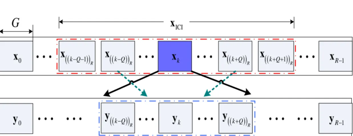
R

Fig. 4.2 An illustration of group-wise detection.

The aforeme complexity, and

rs. ntioned ML-EM algorithm has high computational

hence we use the group-wise method to provide a practical implementation for the ML-EM receiver. N subcarriers are partitioned into R groups, and each group contains G subcarrieS The j th group of subcarriers is given by Gj =

{

jG,…,

(

j+1

)

G−1

}

, for j=0,…,R−1.

Define the j th data group as x_j =_⎣⎡x jG

[

]

,…,x_⎣⎡

(

j+1

)

G−1⎤_⎦⎤_⎦T, the j th ro as y_j =_⎣⎡y jG

[ ]

,…,y⎡⎣

(

j+1

)

G

)

observation g up T 1⎤⎦⎤ − ⎦ , two sets B_j =

{

(

j Q− −1

)

, ,

(

1

)

}

R … j+ +Q R and

(

)

(

)

(

)

{

, ,

}

R … j+Q grouping is demonstrated with

j

D

e of the data groups e.g. the kth data group and illustr in Fig.4.2. The energy of x spreads over the adjacent 2 +1k Q groups (involving k

R . In order to sim on

j Q

= − plify the interpretation, the concept of ated

y itself),

so

{

yj: j∈D is the corresponding set of observation groups. Moreover, the set k

}

{

yj: j∈D k

}

ing d co ig r

nsists of the interference resulted from the spreading energy made b ata groups denoted as

y a set of ne hbo

{

xj: j∈Bk\

{ }

k

}

.

(38)

ML-EM detector and the ICI canceller as depicted in Fig.4.3. During an outer iteration, we diminish the ICI term by subtracting the leakage of other groups from the set of observation groups and then obtain the ICI-reduced signals:

{ } , \ k j j j i i i∈ k = −

∑

B y y H x , for j∈ D_k (4.30)

where the

( )

r s, th entry of H_{j i}_, is given by the

(

jG+r iG, +s

)

th entry of

H

representing an estimate of H for r s, ∈

{

1,…,G−1

}

. H and x come from the output of the EM i detector at the p vious fr the initialization in the beginning. After eliminating the ICI effect, the EM detector is performed by using EM-based channel estimation together with the group-wise method.

When Gibbs sampling is executed, samp re outer iteration or om

les are drawn by applying a ZF sampler. d Every data group, which belongs to the sampler, takes turn by iteration loops to be calculate with the corresponding observation groups

{

yj: j∈D , and thus a large number of samples k

}

are acquired. Then x_k(m-1) is the decided data group at the

(

m 1−

)

th EM iteration defined by an average of the collected samples drawn for the group x_k. And x_k(m-1) is sent back to be an initial data group for the ZF sampler at the mth EM iteration, while x_k( )0 given from the initial setting is an initial data group at the first EM iteration. Going ugh the iteration o Gibbs sampling, we obtain d− sets of detected data groups (for neglecting n0 n sets of 0

burn-in samples). With the o

thro f

(39)

vectors of N transmitted data symbols entireS ly and store up a sequence of probabilities of the final drawing within the

(

m 1−

)

th EM iteration denoted as P(m-1). Because of the probabilities P(m-1), the expected values required in (4.22) can b ulated, and hence derive the channel information ˆ₍_{m 1}₎

e calc

−

a for the

(

m 1−

)

th EM iteration. aˆ₍_{m 1}₋₎ and x(m-1) both provided for the given knowledge at next EM iteration. Besides, a nd

are ( )m

ˆ a x( )m e

yielded as the way described above and become the output of the EM detector at the mth EM iteration. After cancelling the ICI effect,

ar

M can be modified by substituting the updated data

( )m

x into (4.29) via the unit of channel estimation update shown in Fig.4.3. M is replaced by M, and then

H

is calculated as M ΦFa+ ˆ_{( )}_m . Therefore, another outer iteration starts with the given information

H

and x( )m output of the previous outer iteration. The intuition of c bining r design with the group-wise method is presented

from

ou as

the om

below. The data group x contributes most of energy to the ICI-reduced observation groups k

{

yj: j∈D ; thus, we can obtain diversity gains and draw samples for the k

}

kth group data by

nly through x and _k

performing o

{

yj: j∈D . And it is obvious that the f l diversity gain k

}

is attainable when the ICI iminated as well as the value of Q is large enough. Because spreading energy of a group mostly affects the neighboring 2Q groups, i.e the observation group ₍₍ ₎₎

ul effect is co ., mpletely el R k Q+

y is interfered by the data groups

{

xj: j∈

{

k,…

(

k+2Q

)

_R

}

,

so the data groups used for the ICI cancellation should be a set of

,

(

4 +1

)

nce b Q rma groups. However, we can use

(

2Q+3

)

data groups to achieve the comparable perfo y observing the

(40)

experimental trials.

Y

_Y

( )m

x

M

( )0

x

( )m

ˆ

a

Fig. 4.3 The ML-EM receiver for OFDM systems.

雙選擇性通道下正交分頻多工系統中使用馬可夫鏈蒙地卡羅法之基於期望值最大化接收機設計

國

立

交

通 大

學

電

信

工

程

學

系

碩

士

論

文