對於子集合總和問題的最佳化平行的生物分子解的最佳化平行的量子演算法

行政院國家科學委員會專題研究計畫 成果報告

對於子集合總和問題的最佳化平行的生物分子解的最佳化

平行的量子演算法

研究成果報告(精簡版)

計 畫 類 別 ： 個別型

計 畫 編 號 ： NSC 98-2221-E-151-027-

執 行 期 間 ： 98 年 08 月 01 日至 99 年 10 月 31 日

執 行 單 位 ： 國立高雄應用科技大學資訊工程系暨研究所

計 畫 主 持 人 ： 張雲龍

計畫參與人員： 碩士班研究生-兼任助理人員：陳柏樺

碩士班研究生-兼任助理人員：陳姵伶

大專生-兼任助理人員：謝佩如

大專生-兼任助理人員：詹宇翔

大專生-兼任助理人員：潘德聖

報 告 附 件 ： 出席國際會議研究心得報告及發表論文

處 理 方 式 ： 本計畫可公開查詢

中 華 民 國 99 年 10 月 25 日

壹、前言---2

貳、研究目的---2

參、文獻探討---2

肆、研究方法---2

伍、結果與討論---9

陸、參考文獻---9

柒、計畫成果自評---10

壹、前言

In this project, quantum algorithms for solving an instance of the subset-sum

problem are proposed and a NMR experiment for the simplest subset-sum problem to

test our theory is also performed.

貳、研究目的

In this project, an instance of the subset-sum problem can be implemented by our

proposed quantum algorithm. By using nuclear magnetic resonance (NMR) technique,

we perform an NMR experiment for the simplest subset-sum problem to test our

theory.

參、文獻探討

From [1], it was proved that there is an efficient universal quantum Turing machine. But quantum Turing machines could not solve all the NP-complete problems [2]. Quantum query lower bounds for the Hamiltonian circuit, the dominating set and the traveling salesman problem were presented in [3]. Other important works regarding quantum algorithms to solve computational problems include the original version of the quantum Fourier transformation [4].

肆、研究方法

A. Definition of the Subset-sum Problem

Assume that a finite set A is {a

1

, …, am}, where ak is the k

th

element for 1 ≤ k ≤ m.

Definition 4−

−−−1 is applied to denote the subset-sum problem for any a finite set, A.

Definition 4−

−−−1: The subset-sum problem for an m-element finite set, A, is to find a

subset A

1

⊆ A such that the sum of every element in A

1

is exactly b, where b is any

given positive integer.

B. Computational State Space of Quantum Solutions for the Subset-sum Problem

An arbitrary state

ϕ

of a quantum bit is nothing else than a linearly weighted

combination of the following computational basis vectors (4.1):

ϕ

= l

1

⋅

0

+ l

2

⋅

1

= l

1

⋅

1 2

0

1

×













+ l

2

,

1

0

1 2×













where the weighted factors l

1

and l

2

∈ C

2

are the

so-called probability amplitudes, thus they must satisfy | l

1

|

2

+ | l

2

|

2

= 1.

CNOT (controlled NOT) gate is a two-qubit gate and flips the second qubit (the

target qubit) if and only if the first qubit (the control qubit) is one. The CCNOT

(controlled-controlled-NOT) gate is a three-qubit gate and flips the third qubit (the

target qubit) if and only if the first qubit and second qubit (the two control qubits) are

both one.

D. Constructing Quantum Networks for Solving the Subset-sum Problem

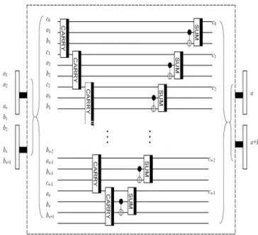
The full addition network is illustrated in Figure 4-1, and can be understood as

follows:

Figure 4-1: Adder network of n quantum bits.

We only reverse all these operations in Figure 4-1 in order to restore every quantum

bit of the three registers to its initial state. This enables us to reuse the same registers

repeatedly.

E. Quantum Algorithms of Solving the Subset-sum Problem

The following quantum algorithm is proposed as quantum implementation on a

physical quantum. The notations used in Algorithm 4-1 below have been denoted in

previous subsections.

Algorithm 4-1: The quantum algorithm is to solve an instance of the subset-sum

problem for any given positive integer b with a finite set A involving m elements of n

bits.

(1) For an initial input

ϕ

₀

=

(

⊗

1_p=n

r

_p0

)

⊗

(

r

₀1

)

⊗

(

⊗

1_q=n+1

b

_1,q

)

⊗

(

b

_n+10

)

⊗

(

⊗

1_j=n

b

_j0

)

⊗

(

, 0

)

1 1 ,j n k j m k= =

a

⊗

⊗

(

, 10

)

1 1 ,= − =

⊗

_{k m j n}

c

_{k j}

⊗

(

⊗

1_k=m

e

_k0

)

⊗

)

(

r

_n+10

⊗

(

1

),

2

m

possible choices of m bits (including all of the possible subsets)

are

ϕ

₁

=

(

⊗

1p=n

I

₂×₂

)

⊗ I

2×2

⊗

(

2 2

)

1 1 × + =

⊗

_{q n}

I

⊗ I

2×2

⊗

(

2 2

)

1 × =

⊗

_{j n}

I

⊗

)

(

⊗

1k=m _,j=n1

I

₂×₂

⊗

(

2 2

)

1 1 ,= × =

⊗

_{k m j n}

I

⊗ H

⊗m

⊗ I

2×2

⊗ H

ϕ

0

=

_m

2

1

)

(

⊗

1_p=n

r

_p0

⊗

)

(

r

₀1

⊗

(

⊗

1_q=n+1

b

_1,q

)

⊗

(

b

_n+10

)

⊗

(

⊗

1_j=n

b

_j0

)

⊗

(

⊗

1_{k=m ,j=n}1

a

_k,j0

)

⊗

)

(

1 1 _{, 1}0 , = − =

⊗

_{k m j n}

c

_{k j}

⊗

(

⊗

1_k=m

(

e

_k0

+

e

_k1

))

⊗

(

r

_n+10

)

⊗

).

2

1

0

(

−

(2)

ϕ

₂

=

(

⊗

1p=n

I

₂×₂

)

⊗ I

2×2

⊗

(

2 2

)

1 1 × + =

⊗

_{q n}

I

⊗ I

2×2

⊗

(

2 2

)

1 × =

⊗

_{j n}

I

⊗

)

(

, 1 1 ,j n k j m k= =

U

⊗

⊗

(

2 2

)

1 1 ,= × =

⊗

k m j n

I

⊗

1

(

⊗

_{k =m}

I

2×2

) ⊗ I

2×2

⊗ I

2×2

ϕ

1

=

m

2

1

)

(

⊗

1_p=n

r

_p0

⊗

(

r

₀1

)

⊗

(

⊗

1_q=n+1

b

_1,q

)

⊗

(

b

_n+10

)

⊗

(

⊗

1_j=n

b

_j0

)

⊗

(

⊗

1_k=m,j=n1

y

_k,j

)

⊗

(

1 1 _{, 1}0

)

,= − =

⊗

_{k m j n}

c

_{k j}

⊗

(

⊗

1_k=m

(

e

_k0

+

e

_k1

))

⊗

(

r

_n+10

)

⊗

),

2

1

0

(

−

where









=

+

⊕

=

=

×

1

if

)

(

0

if

, 1 0 0 , , 2 2 , j k k k j k j k j k

_a

_e

_e

_a

a

I

U

and

.

)

(

0 1 0 , 0 , ,









+

⊕

=

k k j k j k j k

e

e

a

a

y

(3) For s = 1 to m

(3a)

ϕ

_{+s 2}

=

(

⊗

1p=n

I

₂×₂

)

⊗ I

2×2

⊗

(

2 2

)

1 1 × + =

⊗

_{q n}

I

⊗ QA ⊗

1

(

⊗

k =m

I

2×2

) ⊗ I

2×2

⊗ I

2×2 1 + s

ϕ

=

m

2

1

)

(

⊗

1_p=n

r

_p0

⊗

(

r

₀1

)

⊗

(

1 _1,

)

1 q n q= +

b

⊗

⊗

(

b

n+1

)

⊗

(

,

)

1 j s j n j

b +

y

⊗

₌

⊗

(

⊗

1_k=m,j=n1

y

_k,j

)

⊗

(

⊗

_ks+₌1_{m ,j=n}1

c

_{k ,j−1}0

)

⊗

(

⊗

s_k=s,j=n1

c

_k,j−1

)

⊗

)

(

⊗

1_k=s−1,j=n1

c

_k,j−1

⊗

(

⊗

1_k=m

(

e

_k0

+

e

_k1

))

⊗

(

r

_n+10

)

⊗

),

2

1

0

(

−

where QA is

the quantum adder of n bits denoted in Figure 4-1, bn + 1 = ys, n AND bn AND cs, n − 1, cs,

j − 1 = ys, j − 1

AND bj − 1 AND cs, j − 2 for 1 ≤ j ≤ n and ck, j − 1 = yk, j

− 1

AND bj − 1 AND ck,

j − 2 for 1 ≤ k ≤ s − 1 and 1 ≤ j ≤ n.

)

(

⊗

1k=m _,j=n1

I

₂×₂

⊗

(

2 2

)

1 1 ,= × =

⊗

_{k m j n}

I

⊗

1

(

⊗

_{k =m}

I

2×2

) ⊗ I

2×2

⊗ I

2×2

ϕ

m+2

=

_m

2

1

)

(

⊗

1_p=n

r

_p0

⊗

(

r

₀1

)

⊗

(

1 _{1 ,}

)

1 q q n q

b

⊕

b

⊗

_{= +}

⊗

(

b

n+₁

)

⊗

(

)

1 j n j=

b

⊗

⊗

)

(

⊗

1_k=m,j=n1

y

_k,j

⊗

(

⊗

1_k=m,j=n1

c

_k,j−1

)

⊗

(

⊗

1_k=m

(

e

_k0

+

e

_k1

)

⊗

(

r

_n+10

)

⊗

),

2

1

0

(

−

where

b

_j

=

b

_j

+

y

_k,j

and ck, j − 1 = yk, j

− 1

AND bj − 1 AND ck, j − 2 for 1 ≤ k

≤ m and 1 ≤ j ≤ n, and

b

n+₁

is that the last carry is the most significant bit of the

result from the last execution of Step (3a).

(5) For t = 1 to n

(5a)

ϕ

_m+3+t,−1

=

(

2 2

)

1 × =

⊗

p n

I

⊗ I

2×2

⊗

(

2 2

)

1 1 × + + =

⊗

tq n

I

⊗

(

NOT

)

t t q =

⊗

⊗

)

(

⊗

1_q=t-₁

I

_2×2

⊗ I

2×2

⊗

(

22

)

1 × =

⊗

_{j n}

I

⊗

(

⊗

1_{k=m ,j=n}1

I

_2×2

)

⊗

(

⊗

1_{k=m ,j=n}1

I

_2×2

)

⊗

(

⊗

1k =m

I

2×2

) ⊗ I

2×2

⊗ I

2×2

ϕ

m+ t3+−1

=

m

2

1

)

(

⊗

t_p=n

r

_p0

⊗

( ( 1 1, ) ) 0 1 1 p p p t p r ⊕ r •b ⊗ =− −

⊗

)

(

r

₀1

⊗

(

1 _1,

)

1 q t n q

b

+ + =

⊗

⊗

(

b

_{1 t,}

)

⊗

(

1 _1,

)

1 q t q=−

b

⊗

⊗

(

b

n+1

)

⊗

(

)

1 j n j=

b

⊗

⊗

)

(

⊗

1_k=m,j=n1

y

_k,j

⊗

(

⊗

1_k=m,j=n1

c

_k,j−1

)

⊗

(

⊗

1_k=m

(

e

_k0

+

e

_k1

)

⊗

(

r

_n+10

)

⊗

),

2

1

0

(

−

where for 1 ≤ q ≤ t − 1

b

1,_q

is obtained from the execution of the

previous iterations for Step (5a) and for 1 ≤ p ≤ t − 1

r

_p0

⊕

(

r

_p−1

•

b

_1,p

)

is obtained

from the execution of the previous iterations for Step (5b).

(5b)

ϕ

_m+3+t

=

(

⊗

tp+=1n

I

₂×₂

)

⊗

(

CCNOT

)

t t p=

⊗

⊗

(

⊗

1p=t−₁

I

₂×₂

)

⊗ I

2×2

⊗

)

(

⊗

1q=n+₁

I

₂×₂

⊗ I

2×2

⊗

(

22

)

1 × =

⊗

_{j n}

I

⊗

(

⊗

1k=m _,j=n1

I

₂×₂

)

⊗

(

2 2

)

1 1 , = × =

⊗

_{k m j n}

I

⊗

(

⊗

1k =m

I2×2

) ⊗ I

2×2

⊗ I

2×2

ϕ

m+3+t,−1

=

m

2

1

)

(

⊗

t_p+₌1_n

r

_p0

⊗

(

0

(

_{1 1,}

)

t t t

r

b

r

⊕

₋

•

⊗

) ) ( ( 1 1, 0 1 1 p p p t p r ⊕ r •b ⊗ =− −

⊗

(

)

1 0

r

⊗

(

1 _1,

)

1 q t n q

b

+ + =

⊗

⊗

(

b

_{1 t,}

)

⊗

(

1 _1,

)

1 q t q=−

b

⊗

⊗

)

(

b

n+₁

⊗

(

)

1 j n j=

b

⊗

⊗

(

1 1 _,

)

,j n k j m k= =

y

⊗

⊗

(

1 1 _{, 1}

)

, = − =

⊗

_{k m j n}

c

_{k j}

⊗

)

(

(

⊗

1_k=m

e

_k0

+

e

_k1

⊗

(

r

_n+10

)

⊗

),

2

1

0

(

−

where for 1 ≤ p ≤ t − 1

) ( 1 1, 0 p p p r b

r ⊕ − •

is obtained from the execution of the previous iterations for Step

(5b).

EndFor

(6)

ϕ

_{m+ n3+ +1}

=

(

⊗

1p=n

I

₂×₂

)

⊗ I

2×2

⊗

(

)

1 1

NOT

n n q + + =

⊗

⊗

(

⊗

1q=n

I

₂×₂

)

⊗ I

2×2

⊗

)

(

⊗

1_j=n

I

_2×2

⊗

(

⊗

1_{k=m ,j=n}1

I

_2×2

)

⊗

(

⊗

1_{k=m ,j=n}1

I

_2×2

)

⊗

(

⊗

1k =m

I2×2

) ⊗ I

2×2

⊗ I

2×2 n m+3+

ϕ

=

m

2

1

)

)

(

(

1 0 _{1 1,} p p p n p

r

⊕

r

•

b

⊗

_{= −}

⊗

(

r

₀1

)

⊗

(

b

_{1, n+1}

)

⊗

(

1 _{1 ,}

)

q n q=

b

⊗

⊗

)

(

b

n+₁

⊗

(

)

1 j n j=

b

⊗

⊗

(

1 1 _,

)

,j n k j m k= =

y

⊗

⊗

(

1 1 _{, 1}

)

, = − =

⊗

_{k m j n}

c

_{k j}

⊗

)

(

(

⊗

1_k=m

e

_k0

+

e

_k1

⊗

(

r

_n+10

)

⊗

).

2

1

0

(

−

(7)

ϕ

_{m+ n3+ +2}

=

(

⊗

1p=n

I

₂×₂

)

⊗ I

2×2

⊗

(

2 2

)

1 1 × + =

⊗

_{q n}

I

⊗ I

2×2

⊗

(

2 2

)

1 × =

⊗

_{j n}

I

⊗

)

(

⊗

1_{k=m ,j=n}1

I

_2×2

⊗

(

⊗

1_{k=m ,j=n}1

I

_2×2

)

⊗

(

⊗

1k =m

I2×2

) ⊗ CCNOT ⊗ I

2×2

ϕ

m+ n3+ +1

=

m

2

1

)

)

(

(

1 0 _{1 1,} p p p n p

r

⊕

r

•

b

⊗

_{= −}

⊗

(

r

₀1

)

⊗

(

b

_{1, n+1}

)

⊗

(

1 _{1 ,}

)

q n q=

b

⊗

⊗

(

b

n+1

)

⊗

(

⊗

1_j=n

b

_j

)

⊗

(

⊗

1_k=m,j=n1

y

_k,j

)

⊗

(

⊗

1_k=m,j=n1

c

_k,j−1

)

⊗

(

⊗

1_k=m

(

e

_k0

+

e

_k1

)

⊗

)

)

(

(

r

_n0₊₁

⊕

r

_n

•

b

_1,n+1

⊗

).

2

1

0

(

−

(8)

ϕ

_{m+ n3+ +3}

=

(

⊗

1p=n

I

₂×₂

)

⊗ I

2×2

⊗

(

2 2

)

1 1 × + =

⊗

_{q n}

I

⊗ I

2×2

⊗

(

2 2

)

1 × =

⊗

_{j n}

I

⊗

)

(

2 2 1 1 ,= × =

⊗

k m j n

I

⊗

(

2 2

)

1 1 ,= × =

⊗

k m j n

I

⊗

1

(

⊗

_{k =m}

I2×2

) ⊗ I

2×2

⊗

)

2

1

0

(

−

⊕

r

_n+1 2 3+ + + n m

ϕ

=

)

2

1

)

1

((

1 m rn

×

−

+

₍

₍

₎

₎

, 1 1 0 1 p p p n p

r

⊕

r

•

b

⊗

_{= −}

⊗

(

r

₀1

)

⊗

(

b

1, n+1

)

⊗

)

(

1 , 1 q n q=

b

⊗

⊗

(

b

n+₁

)

⊗

(

)

1 j n j=

b

⊗

⊗

(

1 1 _,

)

,j n k j m k= =

y

⊗

⊗

(

1 1 _{, 1}

)

,= − =

⊗

_{k m j n}

c

_{k j}

⊗

)

(

(

⊗

1_k=m

e

_k0

+

e

_k1

⊗

(

r

n+1

)

⊗

).

2

1

0

(

−

(9) Since quantum operations are naturally reversible, the auxiliary quantum bits can

be restored to their initial states by reversing the operations from Steps (7) to (2).

(10) Apply Grover’s operator in Grover’s algorithm to the quantum state vector

generated in Step (9).

(11) At most repeat to execute from Step (2) to Step (10) of

₂

2

m

times.

(12) The answer is obtained with a successful probability of at least

2

1

after a

measurement is finished.

End Algorithm

Lemma 4-1: For a finite set with m elements, n bits of each element in the finite set,

and a given positive integer b, the quantum implementation of the DNA-based

algorithm of solving an instance of the subset-sum problem in Algorithm 4-1 is

equivalent to the oracle work in Grover’s Algorithm, i.e., the target state labeling,

preceding Grover’s searching step.

Proof: It is omitted due to space.

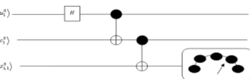
Consider the simplest case of the subset-sum problem with a finite set A

1

= {1} and

any given value b = 1. The size of the first (only) element in the finite set, A

1

, is

represented as a

1, 11

. The size of b (its size is one) is represented as b

1, 11

. The value of

m is equal to one and the value of n is also equal to one. NMR approach has been

widely employed to quantum information processing over past years due to its mature

and well-controllable technology. Although the quantum information processing by

NMR is made on ensembles of nuclear spins, instead of individual spins, NMR has

remained to be the most convenient experimental tool to demonstrate quantum

information processing. We here also adopt this technology to check our theory.

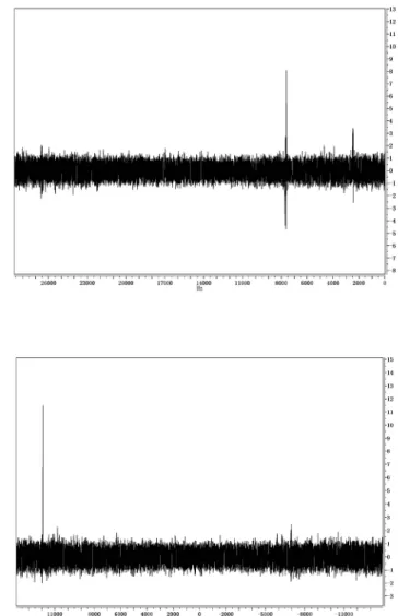
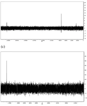
Note that in NMR measurements, the frequencies and phases of NMR signals

could clearly indicate the state the system evolves to after the readout pulses had been

applied. In our experiment, the phases of the reference of

13

C spectra from a thermal

equilibrium were adjusted to be in absorption (i.e., to be positive), and then the same

phase corrections were used to determine the absolute phases of the experimental

spectra of

13

C after the algorithm was accomplished. In our case, the final state was

123 123

( 000

++++

111

) / 2

which means the three qubits are entangled. As the readout

by NMR is a weak measurement, we have no state collapse after the measurement.

Besides, only single quantum coherence can be detected in NMR. As a result, we have

to employ some additional operations to disentangle them for detecting the output

state

( 000

₁₂₃

++++

111

₁₂₃

) / 2

. For this end, we apply a CNOT gate on the second

and first qubits to get the state

( 000

₁₂₃

++++

011

₁₂₃

) / 2

. The second qubit is control

quibte and the first qubit is the target qubit. Then the first qubit can be read out by a s

ingle

ππππ

/ 2

pulse along the x-axis, as shown in Figure 6-1 (a). Similar steps applied

to the second and third quits, respectively, result in the spectrum in Figure 6-1 (b) and

Figure 6-1 (c). It’s evident that the experimental results are in good agreement with

our theoretical prediction.

(a)

(c)

Figure 6-1: Experimental spectra (a)-(c) of the three-qubit solution to the subset-sum

problem after the readout on the first, second and third qubits, respectively.

伍、結果與討論

We have investigated the availability of quantum implementation for an instance of

the subset-sum problem with a finite set involving m elements of n bits. We have also

estimate the complexity of our solution and carried out an experiment by NMR

technology for a simplest example.

陸、參考文獻

[1] E. Bernstein and U. Vazirani. “Quantum Complexity Theory”. Proceedings of the twenty-fifth annual ACM symposium on Theory of computing, pp. 11-20, 1993.

[2] C. H. Bennett, E. Bernstein, G. Brassard and U. V. Vazirani. “Strengths and Weakness of Quantum Computing”. SIAM Journal on Computing, Volume 26, No. 5, pp. 1510-1523, October 1997.

Graph Problems”. Lecture Notes in Computer Science, Volume 2932/2003, pp. 140-150, 2004.

[4] D. Coppersmith. “An approximate Fourier transform useful in quantum factoring”. IBM research report, Technical Report RC 19642, IBM Research Division T.J. Watson Research Center, December 1994. e-print quantph/0201067.

柒、計畫成果自評

We have investigated the availability of quantum implementation for an instance of

the subset-sum problem with a finite set involving m elements of n bits. We have also

estimate the complexity of our solution and carried out an experiment by NMR

technology for a simplest example.

Quantum Algorithms and Mathematical

Representation of Bio-molecular Solutions

for the Clique Problem

in a Finite-dimensional Hilbert Space

Weng-Long Chang1, Ting-Ting Ren2, Mang Feng3 and Jun Luo4, Kawuu Weicheng Lin5, Minyi Guo6, Lai Chin Lu7, Chih-Chiang Wang 8, and Gwo-Jia Jong 9

Abstract—In this paper, it is demonstrated that the DNA-based algorithm [Ho et al. 2005] for solving an instance of the

clique problem to any a graph G = (V, E) with n vertices and  edges and its complementary graph = (V, ) with n vertices and m = (((n * (n – 1)) / 2) – ) edges can be implemented by Hadamard gates, NOT gates, CNOT gates, CCNOT gates, Grover’s operators, and quantum measurements on a quantum computer.

I. QUANTUM ALGORITHMS FOR BIO-MOLECULAR SOLUTIONS OF THE CLIQUE PROBLEM

In this section, the definition of the clique problem and the DNA-based algorithm of solving the clique problem [Ho et al. 2005] will be described. Next, from the DNA-based algorithm of solving the clique problem [Ho et al. 2005], its corresponding quantum algorithm is proposed.

1

A. DEFINITION OF THE CLIQUE PROBLEM

Assume that G is any a graph and G = (V, E), where V is a set of vertices in G and E is a set of edges in G. Also suppose that V is {v1, …, vn} and E is {(va, vb)| va and vb are, subsequently, elements in V}. Assume that |V| is the number of vertices in V and |E| is the number of edges in E. Also assume that |V| is equal to n and |E| is at most (n  (n  1)) / 2 and is equal to  for 1    (n  (n  1)) / 2 . Also suppose that for a graph G its complementary graph G = (V, E ), where E is {(vc, vd)| vc and vd are, respectively, elements in V and (vc, vd) is out of E}. Assume that | E is the number of edges in G and is equal to m that is | equal to (n * (n  1)) / 2  |E|. Mathematically, a clique for a graph G = (V, E) is a complete sub-graph to G. Definition 4-1 cited in [Karp 1975; Garey and Johnson 1979] is used to denote the clique problem of graph G.

Definition 4-1: The clique problem of graph G with n vertices and  edges means finding a maximum-sized clique in G. In Figure 4-1, graph G1 consists of two vertices and an edge. This graph denotes such a problem. All of the cliques in G1 are {v2, v1}, {v1}, {v2} and . The maximum-sized clique for G1 is {v2, v1}. Thus, the size of the clique problem in Figure 4-1 is two. It is indicated in [Karp 1975; Garey and Johnson 1979] that finding a maximum-sized clique is a NP-complete problem and is also an optimization problem, so it can be formulated as a “computational search” problem.

Figure 4-1: the graph G1 of our problem

B. QUANTUM ALGORITHMS FOR COMPUTING THE NUMBER OF ONES TO LEGAL CLIQUES FOR ANY GRAPH

WITH  EDGES AND n VERTICES

The following quantum algorithm is presented to work on the physical quantum computer as proposed by Deutsch [Deutsch 1985] and is employed to compute the number of ones to legal cliques for any graph G with  edges and n vertices. For convenience of presentation, suppose that

,

1 b

x

r

k1

,

,

1 k

c

h

i1, aj,

,

,

1 , j i

f

g

1i, j

,

,

1 0 , 0

z

z

_{i1 j,} 1 , and 1 1 , 1   i i

z

1,5, 7, 8,9_{National Kaohsiung University of Applied Sciences, Kaohsiung City, Taiwan 807-78, Republic of China, E-mail: {}1_{[email protected],} 5

[email protected] , [email protected], 8 [email protected], 9 [email protected] }

2, 3, 4_{Wuhan Institute of Physics and Mathematics, Chinese Academy of Sciences, E-mail: {} 2_{[email protected],} 3_{[email protected],} 4_{[email protected]}} 6

for 1  b  n, 0  k  m, 0  i  n  1, 0  j  i, and 0  a  i  j + 1, subsequently, denote the value of their corresponding quantum bits to be 1. Also suppopse that

,

0 b

x

r

k0

,

,

0 k

c

h

i0, aj,

,

,

0 , j i

f

g

i0, j

,

,

0 0 , 0

z

z

i1 j, 0 , and 0 1 , 1   i i

z

for 1  b  n, 0  k  m, 0  i  n  1, 0  j  i, and 0  a  i  j + 1, subsequently, denote the value of their corresponding quantum bits to be 0. Moreover, the notations used in Algorithm 4-2 below have been denoted in previous subsections. The first parameter w in Algorithm 4-2 is used to represent the maximum size of vertices among legal answers, and its value is passed from the execution of Step (1a) in Algorithm 4-3 in next subsection. To increase the probability of success on measuring the answer from among 2n choices, Grover’s algorithm [Grover 1996] is integrated into the proposed quantum algorithm and is applied to significantly increase the amplitudes of those answers. Grover’s operator is diffusion transform G, which is defined by matrix G as follows: Gi, j = (2n

2

) if i  j and Gi, i = (1+2n 2

).

Algorithm 4-2(w): Quantum algorithms of figuring out the number of one to legal cliques for any a graph G = (V, E) with n vertices and



edges and its complementary graph G = (V, E ) with n vertices and m =

    2 ) 1 (n n edges. (1) For an initial input



= (

1

)



(

0 , 0 1 j i i j n i





z



)



( 1 0 , 0

z

)  ( 0 , 0 0 1 j i i j n i 





g



)  ( 0 , 0 0 1 j i ij n i





f



) 

(

((

)

(

)))

1 0 , , 0 , , 1 1 0 0 1 j i a i j i ja i j n i





h



h



_{    } 

(

)

0 1 k m k

c





(

)

1 0

c

_

)

(



1_km

r

_k1

_

(



1_bn

x

_b0

),

2n possible choices of n bits (including all of the possible cliques) are



0,0 = (H) 

)

(

2 2 0 1   





i n j i

I

_

(

I

_22

)

_

(

22

)

0 0 1    





i n j i

I

_

(

2 2

)

0 0 1    





i n j i

I

_

)))

(

)

((

(

2 2 2 2 1 1 0 0 1       









i n j i a i j

I

I

_

(

2 2

)

1  



k m

I

_

(

I

22

)

_

(

2 2

)

1  



k m

I

_{ Hn}



₌

)

2

1

0

(



 n

2

1

)

(



1_in



0_ji

z

_i,j0 

(

)

1 0 , 0

z



(

)

0 , 0 0 1 j i ij n i





g





(

)

0 , 0 0 1 j i i j n i 





f





)))

(

)

((

(

1, ,0 0 , , 1 1 0 0 1 j i a i j i ja ij n i





h



h



     

(

)

0 1 k m k

c





(

)

1 0

c



(

)

1 1 k m k

r





)).

(

(



1bn

x

b0



x

b1 (2)



1,0 =

(

I

22

)

_

(

2 2

)

0 1   





_{i n j i}

I



(

I

22

)

_

(

22

)

0 0 1    





_{i n j i}

I



(

2 2

)

0 0 1    





_{i n j i}

I



)))

(

)

((

(

1 _{2 2 2 2} 1 0 0 1       









_{i n j i a i j}

I

I

 QEC 



0,0 =

)

2

1

0

(



 n

2

1

)

(



1_in



0_ji

z

_i,j0 

)

(

z

0,01 

(

)

0 , 0 0 1 j i ij n i





g





(

)

0 , 0 0 1 j i ij n i 





f





(

((

)

(

)))

1 0 , , 0 , , 1 1 0 0 1 j i a i j i ja ij n i





h



h



_{    } 

)

)

(

(

1 0 1 k k k m k

c



c



r



  

(

)

1 0

c



(

(

)

)

1 1 j i k m k

r



x



x



 

(

(

)),

1 0 1 b b n b

x



x





where QEC is the quantum circuit in Figure 4-7 and bits xi and xj respectively represent vertices vi and vj in the kth edge, ek = (vi, vj), in G to 1  k  . 2 ) 1 (



   n n (3) For i = 0 to n  1 (4) For j = i down to 0 (4a) 0 , 1 ) ( ) ) 1 ( ( 1 1 0 1 1   _   j i i    =

(

I

22

)

_{ FMNO} 1( ( 1))( ),0 1 0 1 1 ij i    _      = ) 2 1 0 (   n

2

1

)

(

, 0 0 2 l s s l i n s 

z

 







(

(



i_s_1_i1

(

,

)

2 l s j s l

z

 





z

i1,j1



(

c

m



x

i1



z

i,j



z

i1,j2



z

i1,j3







z

i1,i1

)



z

i1,j



(

c

m



x

i1



z

i,j

)



(

)))

0 , 0 1 sl j l 

z



 1

(



_{s i}

(

,

))

0 l s s l

z





(

)

1 0 , 0

z



(

)

0 , 0 1 1 ed de i n d 

g

  







(

((

,

)

1 e d j d e i i d

g

  







)

(

1 , 0 ,j i ij i

x

z

g









(

)))

0 , 0 1 de j e

g





(

(

,

))

0 0 1 e d de i d





g





(

)

0 , 0 1 1 e d de i n d 

f

  







(

((

,

)

1 e d j d e i i d

f

  







(

1 ,, 1

)

0 ,j



i



ijij i

x

h

f



(

)))

0 , 0 1 de j e

f





(

(

,

))

0 0 1 e d de i d





f





)))

(

)

((

(



i_d_1_n1



_e0_d



1_{ade1}

h

_d0_,e,a



h

_d1_,e,0 

(

(

((

,,

)

1 1 1 a e d e d a j d e i i d  

h

  









(

)))

1 0 , ,e d

h



)

)

(

(

, , , 0 1 , ,ji j i j i ji j i

z

h

h

 





 

(

(

(

1, 1 , , 1

)

))

0 , , 1      







a i j

h

i ja

z

i j a

h

i ja 

(

)

1 0 , , j i

h



))))

(

)

((

(

1, ,0 0 , , 1 1 0 1 a d e dea de j e



h



h



     

(

(

((

,,

)

1 1 0 0 1 e d a d e dea i d







 

h





(

))))

1 0 , ,e d

h



(

)

1 k m k

c





(

)

1 0

c



(

)

1 k m k

r





(

(

)),

1 0 1 b b n b

x



x



_

where FMNO is the quantum circuit in Figure 4-8, and for m  k  1 quantum bits

c

k_and

r

k _{are all the results generated from Step (2).}

End For End For (5) 2 1 ,0 ) 1 ( 1nn   = ) 2 1 0 ( zn,w  

(

2 2

)

0 1   





i n j i

I

_

(

I

_22

)

_

(

22

)

0 0 1    





i n j i

I

_

(

22

)

0 0 1    





i n j i

I

_

)))

(

)

((

(

2 2 2 2 1 1 0 0 1       









i n j i a i j

I

I

_

(

2 2

)

1  



k m

I

_

(

I

22

)

_

(

2 2

)

1  



k m

I

_

(

2 2

)

1  



b n

I

0 , 2 ) 1 ( 1nn



=

)

2

1

0

(



 w n z n ,

)

1

(

2

1





)

(

, 0 1 j i i j n i





z





(

)

1 0 , 0

z



(

,

)

0 0 1 j i ij n i





g





)

(

0 0 _, 1 j i ij n i 





f





(

((

)

(

)))

1 0 , , , , 1 1 0 0 1 j i a i j i ja i j n i





h



h



_{    } 

(

)

1 k m k

c





(

)

1 0

c



(

)

1 k m k

r





(

(

)).

1 0 1 b b n b

x



x



_

(6) Since quantum operations are reversible by nature, the auxiliary quantum bits can be restored back to their initial states by reversing all these operations finished by Step (4a) through Step (2).

(7) Apply Grover’s operator in Grover’s algorithm to the quantum state vector generated by Step (6). (8) At most repeat to execute from Step (2) to Step (7) of (

) 2 ( R n 

) times, where the value of R is the number of solutions and can be efficiently computed from quantum counting algorithm in [Imre and Balazs 2005].

(9) The answer is obtained with a successful probability of at least 2 1

after a measurement is finished and return the result to Algorithm 4-3.

EndAlgorithm

Lemma 4-6: Algorithm 4-2 is used to calculate the number of ones (vertices) to legal cliques for any graph G = (V, E) with n vertices and



edges and its complementary graph G = (V, E ) with n vertices and m =

    2 ) 1 (n n edges.

C. QUANTUM ALGORITHMS FOR SOLVING AN INSTANCE OF THE CLIQUE PROBLEM OF ANY GRAPH WITH 

EDGES AND N VERTICES

The following quantum algorithm is applied to solve an instance of the clique problem of any graph G with  edges and n vertices. The notations used in Algorithm 4-3 below have been denoted in previous subsections.

Algorithm 4-3: Quantum algorithms for solving an instance of the clique problem for any a graph G = (V, E) with n vertices and



edges and its complementary graph G = (V, E ) with n vertices and m = 

  2 ) 1 (n n edges. (1) For w = n to 1

(1b) If the answer is obtained from the wth execution of Step (1a) then (1c) Terminate Algorithm 4-3.

End If End For End Algorithm

Lemma 4-7: Algorithm 4-3 is the quantum implementation of Algorithm 4-1 (the DNA-based algorithm) which is equivalent to the oracle work (in the language of Grover’s Algorithm), that is, the target state labeling preceding Grover’s searching step, and is used to solve an instance of the clique problem for any a graph G = (V, E) with n vertices and



edges and its complementary graph G = (V, E ) with n vertices and m = 

  2 ) 1 (n n edges.

II. AN EXAMPLE OF THREE-QUBIT SOLUTION FOR THE CLIQUE PROBLEM

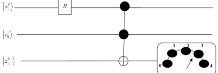
We attempt to test our theory by means of the NMR technique. As with the current technique, the coherent operation using the spatial average approach is only available with three quantum bits, we have to restrict ourselves in the simplest case of the clique problem for a graph G = {V, E}, where V is {v1} and E is {(v1, v1)}. Because the number of vertices in {v1} is one, the number of edges in {(v1, v1)} is also one, and there is no edge in its complementary graph, the value of n is equal to one, the value of  is also equal to one, and the value of m is zero. This is to say that the maximum clique is in fact equal to {v1}. Therefore, Figure 6-1 is the corresponding quantum circuit for the reduced version of Algorithm 4-3 that is to find the answer of the simplest clique problem to the graph

Figure 6-1: The corresponding quantum circuit of the example above

G with {v1} (its vertex) and {(v1, v1)} (its edge). In Figure 6-1, the initial state of solving the simplest case is set to 0 1 , 1

z

1 0

c

x

₁0

.

From Figure 6-1, the Hadamard gate is applied to encode two possible cliques (choices):  and {v1}. In Figure 6-1, the CCNOT gate is employed to check whether  and {v1} are legal cliques or not and to figure out the number of vertices for each legal choice. Since in Figure 6-1, it consists of one quantum bit and two auxiliary quantum bits, it does not need Grover’s operator to increase the amplitude of the answer, and those reversible quantum operations are also unnecessary.

Our experiment is completed on a Varian INOVA 600 NMR spectrometer. The sample is 13

C



labelled

alanine with formula

13 13 13

1

CH

3



2

CH NH

(

2

)



3

COOH

_{, where the three carbons} 13 13

1

C

,

C

,

C

  





_{correspond to the qubits}

I I

1

,



2

,



I

3_, respectively. The J-coupling constants are

J

12



34.79

Hz J

,



23



54.01

Hz J

,



13



1.20

Hz

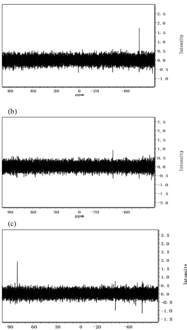
_{. Soft pulses are used to achieve the} selective excitation. The experiment has three main steps as follows. Then the first qubit could be read out by a single



/ 2

pulse along the x-axis, as shown in Figure 6-2(a). Similar steps for the second and the third quantum bits, respectively, result in the spectra in Figure 6-2(b) and Figure 6-2(c). It’s evident that the experimental results are in good agreement with our theoretical prediction.

(b)

(c)

Figure 6-2: Experimental spectra (a)-(c) of a three-qubit solution to the clique problem after the readout is made on the first, second and third qubits, respectively. The single lines in the spectra promise good agreement between our theory and the experiment.

ACKNOWLEDGEMENTS

This work is partly supported by the National Natural Science Foundation of China under Grants No. 10774163, partly by the National Fundamental Research Program of China under Grants No. 2006CB921203, and also partly supported by the National Science Foundation of Republic of China under Grants No. 96-2221-E-151-008-, 96-2218-E-151-004- ,97-2221-E-151-035-, 98-2622-E-151-021-CC3 , and 98-2221-E-151-027-.

Quantum Algorithms and Mathematical

Representation of Bio-molecular Solutions for the

Hitting-set Problem on a Quantum Computer

Weng-Long Chang1, Ting-Ting Ren2, Mang Feng3 and Jun Luo4, Kawuu Weicheng Lin5, Minyi Guo6, Lai Chin Lu7, Gwo-Jia Jong8, and Chih-Chiang Wang9

Abstract—In this paper, it is demonstrated that quantum implementation of bio-molecular solutions to compute the

number of elements in each hitting-set in an instance of the hitting-set problem could be considered as the oracle work in Grover’s algorithm, i.e., the target state labeling, preceding Grover’s searching steps. Finally, for testing our theory, a three-qubit nuclear magnetic resonance (NMR) experiment of solving the simplest hitting-set problem is performed. 2

III. QUANTUM ALGORITHMS OF BIO-MOLECUAR OF THE HITTING-SET PROBLEM

In this section, we will first introduce the definition of the hitting-set problem and the DNA-based algorithm for solving an instance of the hitting-set problem [8]. Then based on bio-molecular solutions for solving an instance of the hitting-set problem [8], its corresponding quantum algorithm is presented.

D. DEFINITION OF THE HITTING-SET PROBLEM

Assume that a finite set S is {un, , u1}, where ui is the ith element in S with 1  i  n. |S| is denoted as the number of elements

in S and |S| is equal to n. Suppose that a collection C is a set of subsets of the finite set S, denoted by {C1, , Cm}, where Cj is the

jth element in C with 1  j  m. |C| is denoted as the number of subsets in C and |C| is equal to m. Mathematically, a hitting-set is to find whether there is a subset S1  S such that S1 contains at least one element from each subset in C. Definition 4-1 cited in [9] is applied to denote the hitting-set problem, which is an NP-complete problem [9].

Definition 4-1: The hitting-set problem with an n-element finite set S and an m-element collection C of subsets for S means finding a minimum-sized hitting-set.

As an example, we consider a simple case in Figure 4-1, where the finite set S is {2, 1} and the collection C is {{1}}. The two sets define a hitting-set problem. In Figure 4-1, there are two hitting sets that are, respectively, {1} and {1, 2}. From Definition 4-1, the answer (a minimum-sized hitting-set) of the hitting-set problem for S and C in Figure 4-1 is {1}.

S = {2, 1} and C = {{1}}

Figure 4-1: A finite set S and a collection C of subsets for S.

E. QUANTUM ALGORITHMS FOR CALCULATING THE NUMBER OF ONES TO LEGAL HITTING SETS

The following quantum algorithm is proposed to work on the physical quantum computer proposed by Deutsch [6] and is applied to figure out the number of ones to legal hitting sets in the hitting-set problem with an n-element finite set S and an

m-subset collection C. For convenience of presentation, it is supposed that

u

1q

,

,

1 ,q k

r

c

1k

,

,

1 , , aj i

h

f

i1, j,0

,

,

1 0 , , j i

g

1,5, 7, 8,9_{National Kaohsiung University of Applied Sciences, Kaohsiung City, Taiwan 807-78, Republic of China, E-mail: {}1_{[email protected],} 5