Genetic Association Studies of Adult-Onset Diseases Using the Case-Spouse and Case-Offspring Designs

(1)

Volume 158

Number 11

December 1, 2003

EPIDEMIOLOGY

Sponsored by the Society for Epidemiologic Research Published by Oxford University Press

SPECIAL ARTICLES AND COMMENTARY

Genetic Association Studies of Adult-Onset Diseases Using the Case-Spouse and

Case-Offspring Designs

Wen-Chung Lee

From the Graduate Institute of Epidemiology, College of Public Health, National Taiwan University, Taipei, Taiwan, Republic of China.

Received for publication August 7, 2002; accepted for publication June 10, 2003.

Genetic studies of complex human diseases rely heavily on the family-based association paradigm. However, recruiting parents or siblings can be a difficult task in practice. The author proposes two alternatives, the case-spouse and the case-offspring designs, that are to be analyzed by the mating disequilibrium test. Two assumptions are required: 1) the marker genotype frequencies at conception should be the same for both sexes; and 2) there is no selective attrition of marker allele(s) through gestation and over time. Within this setting, the case-spouse and the case-offspring studies are valid designs, even if only one sex can get the disease, even if cases/spouses/offspring all have different risk factor profiles, and even under assortative mating. If the population is stratified and there is intermarriage between strata, one can type additional null markers across the genome for an admixture correction. The number of families required in a case-spouse design is almost identical to that in a case-parents design. For the case-offspring study with one offspring per family, the number of families should be doubled. Because of the ease in recruiting control subjects, the case-spouse and the case-offspring designs are viable alternatives for genetic association studies of adult-onset diseases.

epidemiologic methods; genetics; polymorphism, single nucleotide

Abbreviations: df, degree of freedom; MDT, mating disequilibrium test; PDT, pedigree disequilibrium test; TDT, transmission/ disequilibrium test.

Editor’s note: An invited commentary on this article

appears on page 1033, and the author’s response appears on page 1036.

It has been argued that the genetic analysis of complex human diseases will rely more and more on the epidemio-logic association paradigm (1, 2). In particular, the applica-tion of the transmission/disequilibrium test (TDT) in a

case-parents study has received much attention (3, 4). For a marker with two alleles, the TDT compares the number of heterozygous parents who transmit one allele with the number of heterozygous parents who transmit the other allele to the affected offspring. Because the comparison is within family, it is not affected by population stratification, which can produce an excess of false positive results in a conventional case-control study (4).

Reprint requests to Dr. Wen-Chung Lee, Graduate Institute of Epidemiology, National Taiwan University, No. 1, Jen-Ai Road, 1st Section, Taipei 100, Taiwan, Republic of China (e-mail: wenchung@ha.mc.ntu.edu.tw).

(2)

Although it successfully removes the population stratifica-tion bias, using parents as the control group can create a problem of its own. Parents may have died already, making it impossible to genotype them. This is particularly true when the disease under study has an age at onset in adult-hood or older, such as non-insulin-dependent diabetes, cardiovascular diseases, Alzheimer’s disease, many forms of cancers, and so on. Without parental genotypes, one cannot trace the transmission of the alleles from parents down to their offspring. Assuming noninformative missingness, several authors (5–7) have proposed methods to tackle this missing-parent problem. However, the assumption can be violated in several ways (5–8).

A case-sibling study using siblings as the control group is an alternative design option (9–11). It is true that siblings were still alive more often than parents were when cases were recruited. However, siblings of an adult case normally do not live together with the case, making it difficult to recruit them for study. Furthermore, it is possible that some of the cases in the study do not have siblings at all.

In this paper, I will propose two alternatives, the case-spouse and the case-offspring designs, that recruit the spouses and the offspring, respectively, as the control group. These designs are particularly useful for genetic study of adult-onset diseases, because of the ease in recruiting the control subjects; an adult normally will get married and live together with his/her mate and, if any, with their child(ren). A new test will be proposed, the mating disequilibrium test (MDT), to analyze the case-spouse and case-offspring data. The conditions for a MDT to be a valid test for genetic asso-ciation with a disease-susceptibility gene will be discussed and be examined through computer simulation. (In this paper, a disease-susceptibility gene refers to a gene that will by itself influence the risk of disease, or that will predispose a subject to risk factor(s) of the disease and thereby indi-rectly influence the disease risk.) Finally, a power formula for a genome-wide scan using spouse and case-offspring designs will be given, and the number of families required will be compared with that required using the case-parents design.

THE CASE-SPOUSE AND THE CASE-OFFSPRING DESIGNS

Suppose that a sample of n (i = 1, …, n) cases has been recruited. Genotyping has been done at a particular marker locus with two alleles, M and m. (Note that this paper does not consider markers in the sex chromosome.) For the ith case, the M-allele count is denoted as Ci. The spouse of the

ith case, if available for study, is also genotyped with an

M-allele count of Si. If the spouse of the ith case is missing but his/her offspring is/are available for genotyping, one calcu-lates the Oi, the average M-allele count of the offspring of the

ith case, and then imputes the M-allele count of the missing

spouse by . (The imputation is based on the obvious fact that

Note that defined in this way can become negative some-times and should not be reset to zero should that happen). The difference of the M-allele count between the ith case and his/her spouse (or the imputed spouse) is denoted as . The Dis are the basic data to be analyzed.

The following two assumptions are invoked in the case-spouse and the case-offspring studies. 1) The marker geno-type frequencies at conception should be the same for both sexes. This assumption is likely to be met in practice because of random segregation of sex chromosomes and autosomes. 2) There is no selective attrition of marker allele(s) through gestation and over time. In other words, the marker studied should not be in linkage disequilibrium with a gene, or be a gene itself, that affects survival through gestation or over time. This is the same assumption invoked in the case-parents and the case-sibling studies (12).

If the validity of the assumptions is a concern, one should check the genotypes of the unaffected individuals recruited in a study (the sibling in the case-sibling study, the spouse in the case-spouse study, and the offspring in the case-offspring study) to see if the frequencies vary over sex or age.

Under the null hypothesis that the marker is not genetically associated with the disease in question (by genetic associa-tion, we mean that the marker is in linkage disequilibrium with a disease-susceptibility gene or that the marker is a disease-susceptibility gene itself), the expected value of Di will be zero if both assumptions are met and if the study population is a homogeneous population or a stratified popu-lation but mating is restricted to subjects in the same stratum. Note that the above assumptions suffice to ensure that the spouse and the offspring of a case are his/her legitimate controls. The expected value of Di will be zero, even if only one sex can get the disease, even if cases/spouses/offspring all have different risk factor profiles, and even under assorta-tive mating.

THE MATING DISEQUILIBRIUM TEST

With the assumptions stated above, the following X2

statistic is a valid test for genetic association with a disease-susceptibility gene:

Under the null hypothesis, X2_{is asymptotically a chi-square}

distribution with 1 degree of freedom (df). The MDT is based on this statistic.

The data of a case-spouse study have the same structure as the data of a pair-matched case-control study, and they can alternatively be analyzed using a logistic regression based on

Dis (13). It can be shown that the above X2_{is the efficient}

score statistic of such a logistic model. If the data consist

Sî = 2Oi–Ci E Ci+Si 2 ---    _{E O} i ( ). = Sî Di = Ci–Si(or Di=Ci–Sî) X2 Di⁄n i=1 n

∑

–E D( )i 2 Var D( ) ni ⁄ ( ) ⁄ = Di⁄n i=1 n

∑

–0 2 Di 2 i=1 n

∑

⁄n2     ⁄ = Di i=1 n

∑

   2 Di 2 i=1 n

∑

⁄ . =

(3)

exclusively of pairs of cases and their single offspring, it can also be shown that the above X2_{is algebraically the same as}

the 1-TDT statistic proposed by Sun et al. (5), except that the 1-offspring now plays the role of the 1-parent in the 1-TDT. Monte-Carlo simulation was performed to study the empirical type I error rates of the MDT. The study popula-tion was assumed to be composed of two strata (the first stratum constitutes 40 percent, and the second, 60 percent). The two strata do not intermix. Disease prevalences were assumed to be different between the sexes. In the first stratum, the prevalences were 3 × 10–5 for males and 2 × 10–6

for females. In the second stratum, the prevalences were 3 × 10–5 · r for males and 2 × 10–6_{· r for females, where r is the}

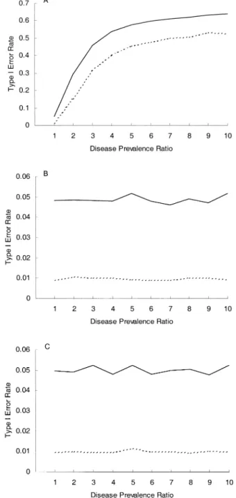
disease prevalence ratio between the second and the first strata. The effect of varying the extent of population stratifi-cation was examined for r = 1, …, 10. In each round of simu-lation, the M-allele frequencies for the first and the second strata were generated by taking two numbers at random from the interval (0.05, 0.95). (This represents an average of 0.3, in the absolute allele-frequency differences between these two strata.) Both random mating and assortative mating within the stratum were considered. For the assortative mating, 90 percent of the subjects in a given stratum performed random mating, and the remaining 10 percent performed mating strictly within the same genotype. (To make sense of this contrived scenario, one can think of a genetic marker that is associated with, e.g., body height. In the population, 90 percent of the subjects are not choosy about the physique of their potential mates. Yet, the remaining 10 percent won’t mate unless they find someone with similar height.) A total of 200 cases were recruited from the population at large. Because the disease prevalence is very low, it was assumed that these cases were from different families. Control subjects were recruited according to the conventional case-control design (200 control subjects), the case-spouse design, and the case-offspring design (three offspring per family), respectively. The Armitage trend test (14) was applied for the case-control design. (Sasieni (15) has pointed out that the usual Pearson chi-square statistic comparing allele frequencies between cases and controls is inappropriate when Hardy-Weinberg equilibrium does not hold.) The MDT was applied for the case-spouse and the case-offspring designs. The nominal α levels were set in turns at 0.05 and 0.01. Ten thousand simulations were performed for each scenario created.

Figure 1 presents the results of random mating within the stratum. It can be seen that the case-control study produces grossly inflated type I error rates for the disease prevalence ratio of >1 (figure 1, part A), whereas the case-spouse (figure 1, part B) and case-offspring (figure 1, part C) designs main-tain the nominal α levels in the range of disease prevalence ratios that were studied. The same conclusion can be drawn when there is assortative mating within the stratum (results not shown).

CORRECTION FOR POPULATION ADMIXTURE

In the above, we have seen that the MDT can be a valid test for genetic association, when the study population is a homo-geneous one or when it is stratified but mating is restricted to

subjects of the same stratum. In real practice, however, a nonnegligible fraction of marriages may occur between subjects belonging to different strata. Under such a model of “population admixture,” the spouse is no longer a “perfect match” for the case. There is no guarantee that the expected value of Di under the null will be zero, because we are now comparing two subjects belonging to different strata with possibly different marker allele frequencies. Therefore, the FIGURE 1. Type I error rates (nominal error rate: solid line, 0.05; dashed line, 0.01) in a stratified population with random mating within the stratum, for a case-control study (A), a case-spouse study (B), and a case-offspring study (three offspring per family) (C).

(4)

MDT is expected to produce an excess of false positive results.

I suggest using a principle of multiplicative scaling of chi-square distribution proposed by Reich and Goldstein (16) for a correction of the MDT statistic. (Their method was proposed originally to correct the allelic chi-square statistic of a case-control design, under the model of “population stratification.”) To be precise, a number of markers unlinked to (or in linkage equilibrium with) the foregoing candidate marker were also genotyped in the same set of cases and spouses (offspring). (These “null markers” are to be chosen at random throughout the whole genome, so that it is unlikely that any one is tightly linked to a disease-suscepti-bility gene.) The average of the MDT statistics across the null markers provides a measure of the amount of admixture. By dividing the candidate MDT by this average (the prin-ciple of multiplicative scaling of chi-square distribution (16)), one can obtain a p value that corrects for admixture.

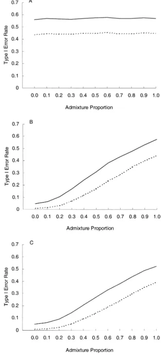
Monte-Carlo simulation was performed to study the effec-tiveness of such an admixture correction. The two-strata population in the previous section was considered again (with a disease prevalence ratio of 5). This time, however, varying degrees of admixing between strata were allowed (admixture proportions of 0.0, 0.1, …, 1.0 were studied). An admixture proportion of 0.0 implies random mating within the stratum but no intermarriage between strata. At the other extreme of an admixture proportion of 1.0, there is random mating in the population at large. In the middle, for example, an admixture proportion of 0.3, 30 percent of the population mate randomly without regard to population stratification, and the remaining 70 percent mate only within the stratum. In addition to the candidate marker, a total of 50 null markers were typed. The allele frequencies for the candidate marker as well as for the null markers in the first and the second strata were generated by taking random numbers from (0.05, 0.95) in each round of simulation (one pair of numbers for the candidate marker plus 50 pairs of numbers for the 50 null markers within each simulation). For the case-control study, the Armitage trend statistic of the candidate marker was divided by the average of the same statistics of the 50 null markers. For the case-spouse and the case-offspring studies, the candidate-marker MDT was divided by the average MDT of the 50 null markers. All the other simulation settings are the same as in the previous section.

Figure 2 presents the results without admixture correction (candidate-marker Armitage trend test and MDT, without being divided by the corresponding statistics of the null markers). It can be seen that the case-control study (figure 2, part A) produces grossly inflated type I error rates, irrespec-tively of the admixture proportion in the population. Without admixture correction, the case-spouse (figure 2, part B) and the case-offspring (figure 2, part C) studies also produce inflated type I error rates. The inflation becomes more intol-erable as the admixture proportion becomes larger.

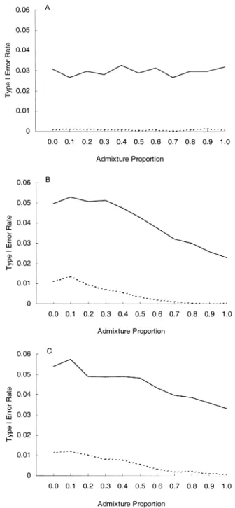
Figure 3, part A, presents the simulation results for the conventional case-control study, corrected for population admixture. It can be seen that, by typing null markers and applying the principle of multiplicative scaling of chi-square distribution, one can indeed correct the inflation of type I error rates (compare part A of figure 3 with part A of figure

2). However, the correction leads to an extremely conserva-tive test (empirical type I error rate = ~0.03 at α = 0.05 and ~0.0008 at α = 0.01). By contrast, the corrections in the case-spouse (figure 3, part B) and the case-offspring (figure 3, part C) studies lead to type I error rates that are very close to the respective nominal α level, at least for the mild-to-moderate amount of intermarriage between strata (admixture proportion < ~0.3).

FIGURE 2. Effects of not performing admixture correction (nominal error rate: solid line, 0.05; dashed line, 0.01), for a case-control study (A), a case-spouse study (B), and a case-offspring study (three off-spring per family) (C).

(5)

POWER FORMULA AND NUMBER OF FAMILIES REQUIRED

I derive the power formula for the case-spouse (case-offspring) study under the assumption of a homogeneous random-mating population with Hardy-Weinberg equilib-rium. The derivation follows closely the approaches of Knapp (17) and of Chen and Deng (18) in their derivations of

the power of TDT. The first step is the enumeration of “family type” or “family class.” The specific marker geno-type of the case, together with that of his/her spouse (or offspring), constitutes a specific family type. Assume that there are a total of K (j = 1, …, K) different types of families. Let Qj denote the probability that a family is of type j, and let

Dj denote the difference of M-allele counts between the case and his/her (imputed) spouse for a family of type j. (To derive the power formula, family types with the same Dj can be pooled together as one family class, with the class proba-bility being the sum of the probabilities of the contributing family types. Chen and Deng (18) described an efficient algorithm to calculate the class probabilities.) Further, let

Let us consider

The distribution of X (under either H₀ or H₁) can be approxi-mated by a normal distribution. Using the multivariate delta method (19), one can show that, for large n, such a distribu-tion has a mean of

and a variance of

Let zw denote the w quantile of a standard normal distribu-tion. Then,

To compare the powers of the MDT in the case-spouse (case-offspring) design and the TDT in the case-parents design, one assumes that the marker is a disease-susceptibility gene per se (two alleles, D and d) and that the same modes of inheritance as used by Knapp (17) were considered (ψ1:

geno-type relative risk of Dd over dd; ψ2: DD over dd): 1) the

multi-plicative model (ψ1 = γ and ψ2 = γ2), 2) the additive model

(ψ1 = γ and ψ2 = 2γ according to Camp’s definition (20) of

additive mode of inheritance for the sake of comparability), 3) the recessive model (ψ1 = 1 and ψ2 = γ), and 4) the dominant

model (ψ1 = ψ2 = γ). The test was two sided with the α level

set at 10–7. This corresponds to α = 5 × 10–8_{for the}

genome-wide one-sided TDTs used by Risch and Merikangas (1). (If allele D is positively associated with the disease and α is FIGURE 3. Effects of performing admixture correction (nominal

error rate: solid line, 0.05; dashed line, 0.01), for a case-control study (A), a case-spouse study (B), and a case-offspring study (three off-spring per family) (C).

e₁ Q_jD_j j=1 K

∑

= e₂ Q_jD_j2, j=1 K

∑

= , e₃ QjDj 3 j=1 K

∑

= and e₄ QjDj 4 . j=1 K

∑

= , X _i Di 1 = n

∑

Di 2 i=1 n

∑

⁄ . = µ n e⋅ 1 e₂ ---≈ σ2 1 e3 e₂2 ----      e₁ 1 4 --- e4 e2 2 – e₂3 ---      e₁2. ⋅ + ⋅ – ≈ Power of the MDT Pr Z –z1–α 2⁄ –µ σ ---<     _{Pr Z} z₁_–_{α 2}_⁄ –µ σ --->    _. + ≈

(6)

small, the power of one-sided TDT for allele D with a type I error rate of α is very near the power of two-sided TDT with a type I error rate of 2α.) For each combination of mode of inheritance, risk parameter γ (γ = 1.5, 2, 4), and allele frequency P of D in the source population (P = 0.01, 0.1, 0.5, 0.8), the numbers of families required to achieve 80 percent power for the MDT in a spouse design and a case-offspring (number of case-offspring: 1, …, 5) design were calcu-lated by solving the above power formula using a bisection method (a root-finding method (21)). To check the precision of power approximation, 100,000 simulated data sets at the above-calculated sample sizes were generated. For each round of simulation, the MDT was calculated, and the true power was estimated as the proportion of simulations rejecting the null hypothesis at α = 10–7_{. (The sample size for the}

case-spouse design can be calculated alternatively using the method of Julious and Campbell (22) for matched ordinal data. However, simulation shows that the method will lead to a gross underestimation of sample size sometimes (results not shown)).

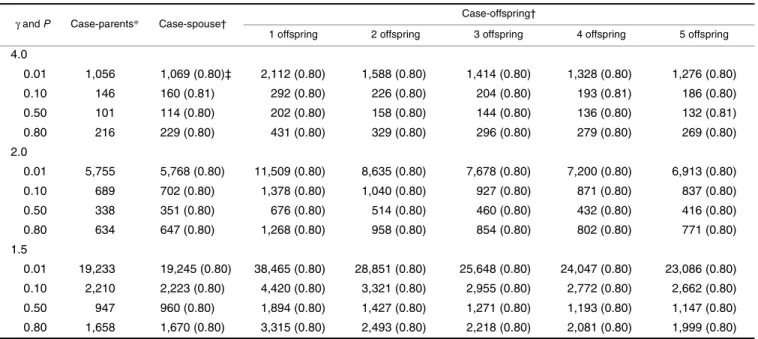
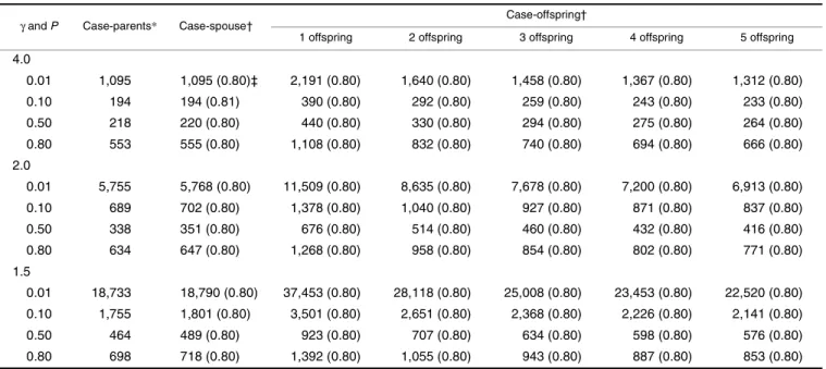
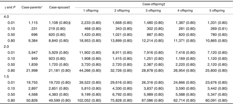
Tables 1, 2, 3, and 4 present the number of families required to achieve 80 percent power by the MDT under various conditions. The empirical powers based on simula-tions (in parenthesis) match very well with the expected value of 0.80, indicating that the power formula presented in this paper is quite accurate. For the purpose of comparison, these tables also present the numbers of families required by a genomewide TDT scan, which numbers were taken from table 3 of Knapp (17). It can be seen that the differences in numbers of families required between the case-spouse and

the case-parents designs are inconsequential (slightly higher in the multiplicative, additive, and recessive modes of inher-itance and slightly lower in the dominant mode of inherit-ance for the spouse design compared with the case-parents design), whereas the number of families required is higher for the offspring design compared with the case-spouse design. As the number of offspring increases, the number of families required for a case-offspring design decreases. These findings are as expected, because imputed data were used for calculating the MDT in a case-offspring design, and the more offspring a case has, the more precise the imputation of his/her missing spouse can be. Tables 1, 2, 3, and 4 suggest that the number of families should be doubled with single-offspring families. If five offspring in a family are available for study, a case-offspring study is comparable with a case-spouse study in terms of the number of families required.

TWO-DEGREE-OF-FREEDOM LIKELIHOOD RATIO TESTS

The above MDT for case-spouse data and the TDT for case-parents data are both based on a 1-df chi-square distri-bution. However, Weinberg et al. (23) and Schaid (24) had shown that a 2-df likelihood ratio test can deliver better power under either a recessive or a dominant mode of inher-itance for case-parents data. A 2-df likelihood ratio test for case-spouse data can also be performed as follows. Let C_1i = 1 if the ith case has genotype Mm, and C_1i = 0 if otherwise. Furthermore, let C_2i = 1 if the ith case has genotype MM, and TABLE 1. Number of families required to achieve 80% power at α = 10–7_{for the various designs under the multiplicative mode of}

inheritance

* The number of families required for the case-parents design (using the transmission/disequilibrium test) was taken from table 3 of Knapp (17).

† Using the mating disequilibrium test.

‡ Numbers in parentheses, empirical powers based on 100,000 simulations.

γ and P Case-parents* Case-spouse† Case-offspring†

1 offspring 2 offspring 3 offspring 4 offspring 5 offspring

4.0 0.01 1,056 1,069 (0.80)‡ 2,112 (0.80) 1,588 (0.80) 1,414 (0.80) 1,328 (0.80) 1,276 (0.80) 0.10 146 160 (0.81) 292 (0.80) 226 (0.80) 204 (0.80) 193 (0.81) 186 (0.80) 0.50 101 114 (0.80) 202 (0.80) 158 (0.80) 144 (0.80) 136 (0.80) 132 (0.81) 0.80 216 229 (0.80) 431 (0.80) 329 (0.80) 296 (0.80) 279 (0.80) 269 (0.80) 2.0 0.01 5,755 5,768 (0.80) 11,509 (0.80) 8,635 (0.80) 7,678 (0.80) 7,200 (0.80) 6,913 (0.80) 0.10 689 702 (0.80) 1,378 (0.80) 1,040 (0.80) 927 (0.80) 871 (0.80) 837 (0.80) 0.50 338 351 (0.80) 676 (0.80) 514 (0.80) 460 (0.80) 432 (0.80) 416 (0.80) 0.80 634 647 (0.80) 1,268 (0.80) 958 (0.80) 854 (0.80) 802 (0.80) 771 (0.80) 1.5 0.01 19,233 19,245 (0.80) 38,465 (0.80) 28,851 (0.80) 25,648 (0.80) 24,047 (0.80) 23,086 (0.80) 0.10 2,210 2,223 (0.80) 4,420 (0.80) 3,321 (0.80) 2,955 (0.80) 2,772 (0.80) 2,662 (0.80) 0.50 947 960 (0.80) 1,894 (0.80) 1,427 (0.80) 1,271 (0.80) 1,193 (0.80) 1,147 (0.80) 0.80 1,658 1,670 (0.80) 3,315 (0.80) 2,493 (0.80) 2,218 (0.80) 2,081 (0.80) 1,999 (0.80)

(7)

TABLE 2. Number of families required to achieve 80% power at α = 10–7_{for the various designs under the additive mode of}

inheritance

4.0 0.01 1,095 1,095 (0.80)‡ 2,191 (0.80) 1,640 (0.80) 1,458 (0.80) 1,367 (0.80) 1,312 (0.80) 0.10 194 194 (0.81) 390 (0.80) 292 (0.80) 259 (0.80) 243 (0.80) 233 (0.80) 0.50 218 220 (0.80) 440 (0.80) 330 (0.80) 294 (0.80) 275 (0.80) 264 (0.80) 0.80 553 555 (0.80) 1,108 (0.80) 832 (0.80) 740 (0.80) 694 (0.80) 666 (0.80) 2.0 0.01 5,755 5,768 (0.80) 11,509 (0.80) 8,635 (0.80) 7,678 (0.80) 7,200 (0.80) 6,913 (0.80) 0.10 689 702 (0.80) 1,378 (0.80) 1,040 (0.80) 927 (0.80) 871 (0.80) 837 (0.80) 0.50 338 351 (0.80) 676 (0.80) 514 (0.80) 460 (0.80) 432 (0.80) 416 (0.80) 0.80 634 647 (0.80) 1,268 (0.80) 958 (0.80) 854 (0.80) 802 (0.80) 771 (0.80) 1.5 0.01 18,733 18,790 (0.80) 37,453 (0.80) 28,118 (0.80) 25,008 (0.80) 23,453 (0.80) 22,520 (0.80) 0.10 1,755 1,801 (0.80) 3,501 (0.80) 2,651 (0.80) 2,368 (0.80) 2,226 (0.80) 2,141 (0.80) 0.50 464 489 (0.80) 923 (0.80) 707 (0.80) 634 (0.80) 598 (0.80) 576 (0.80) 0.80 698 718 (0.80) 1,392 (0.80) 1,055 (0.80) 943 (0.80) 887 (0.80) 853 (0.80)

TABLE 3. Number of families required to achieve 80% power at α = 10–7_{for the various designs under the recessive mode of}

inheritance

γ and P _parents*Case- Case-spouse†

Case-offspring†

1 offspring 2 offspring 3 offspring 4 offspring 5 offspring 4.0 0.01 4,344,070 4,398,630 (0.80)‡ 8,671,140 (0.80) 6,534,940 (0.80) 5,822,855 (0.80) 5,466,807 (0.80) 5,253,176 (0.80) 0.10 5,631 6,179 (0.80) 11,108 (0.80) 8,646 (0.80) 7,825 (0.80) 7,414 (0.80) 7,167 (0.80) 0.50 207 242 (0.80) 405 (0.80) 324 (0.80) 297 (0.80) 283 (0.80) 275 (0.80) 0.80 259 282 (0.80) 512 (0.80) 397 (0.80) 358 (0.80) 339 (0.80) 327 (0.80) 2.0 0.01 38,654,522 38,818,617 (0.80) 77,257,476 (0.80) 58,038,104 (0.80) 51,631,627 (0.80) 48,428,383 (0.80) 46,506,434 (0.80) 0.10 45,071 46,711 (0.80) 89,646 (0.80) 68,183 (0.80) 61,027 (0.80) 57,448 (0.80) 55,301 (0.80) 0.50 957 1,037 (0.80) 1,894 (0.80) 1,465 (0.80) 1,322 (0.80) 1,251 (0.80) 1,208 (0.80) 0.80 851 891 (0.80) 1,691 (0.80) 1,291 (0.80) 1,157 (0.80) 1,091 (0.80) 1,051 (0.80) 1.5 0.01 154,174,890 154,503,292 (0.80) 308,246,348 (0.80) 231,374,878 (0.80) 205,751,035 (0.80) 192,939,108 (0.80) 185,251,950 (0.80) 0.10 174,694 177,976 (0.80) 348,375 (0.80) 263,180 (0.80) 234,780 (0.80) 220,580 (0.80) 212,060 (0.80) 0.50 3,099 3,243 (0.80) 6,155 (0.80) 4,699 (0.80) 4,214 (0.80) 3,971 (0.80) 3,826 (0.80) 0.80 2,356 2,422 (0.80) 4,694 (0.80) 3,558 (0.80) 3,179 (0.80) 2,990 (0.80) 2,876 (0.80)

(8)

C_2i = 0 if otherwise. S_1i and S_2i are defined similarly for the

ith spouse. Assuming a logistic model, one finds that the

conditional likelihood of the data is

where D_1i = C_1i – S_1i and D_2i = C_2i – S_2i are the differences in genotype counts for case versus spouse in the ith pair (13). A standard logistic regression program can be used to obtain the maximum likelihood estimates, and . The deviance statistic for this model is

and the deviance statistic for the null model is G0 = 2n × log

2. Consequently, the 2-df likelihood ratio test for testing H₀ (β1 = β2 = 0) is based on G0 – G1.

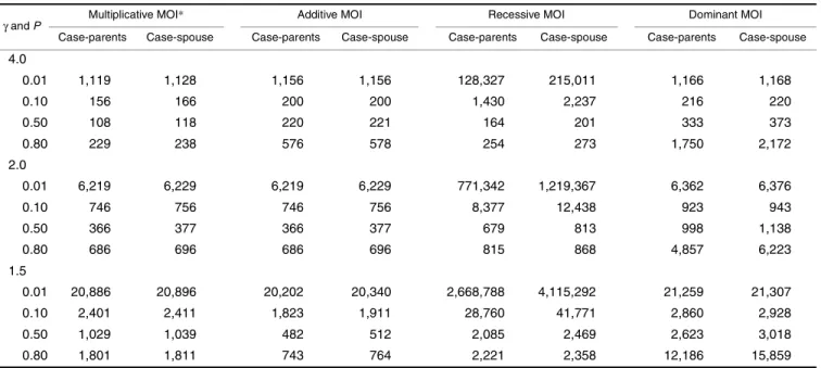
Using the method of Longmate (25), I calculate the number of families required by the 2-df likelihood ratio test to achieve 80 percent power at α = 10–7 _{for the case-parents}

and the case-spouse studies under various modes of inherit-ance (table 5). It can be seen that the number of families required by the case-spouse study is larger than that needed by the case-parents study, but the difference is

inconspic-uous. Compared with the 1-df tests (tables 1, 2, 3, and 4), we see as expected that the 2-df likelihood ratio tests can indeed reduce the number of families required to achieve the same power in both the case-parents and the case-spouse studies, under the recessive mode of inheritance and several occa-sions of dominant mode of inheritance.

DISCUSSION

It is of interest to compare the MDT with the pedigree disequilibrium test (PDT) proposed by Martin et al. (26, 27). The PDT considers the previous (parents) and the same (sibings) generations from the perspective of a case, whereas the MDT traces family trees horizontally and/or downward to the same generation (spouses) and/or to the next one (offspring). Like the PDT, the MDT is also a valid test for genetic association (linkage and association). It will main-tain the nominal α level for markers linked to but not associ-ated with a putative disease-susceptibility gene.

In practice, we usually have various configurations of families in a study, with the following hierarchy: 1) geno-type available for both parents; 2) genogeno-type available for unaffected sibling(s) but not for both parents; 3) genotype available for the spouse but not for the unaffected sibling and not for both parents; and 4) genotype available for offspring but not for spouse, not for unaffected sibling, and not for both parents. The method described in this paper can easily be extended to deal with all these families, by redefining Di, respectively, as: 1) the number of transmitted

M alleles minus the number of nontransmitted M alleles;

TABLE 4. Number of families required to achieve 80% power at α = 10–7_{for the various designs under the dominant mode of}

inheritance

4.0 0.01 1,115 1,108 (0.80)‡ 2,233 (0.80) 1,668 (0.80) 1,480 (0.80) 1,387 (0.80) 1,331 (0.80) 0.10 231 219 (0.80) 468 (0.80) 343 (0.80) 302 (0.80) 281 (0.80) 269 (0.81) 0.50 696 620 (0.80) 1,420 (0.80) 1,021 (0.80) 887 (0.80) 820 (0.80) 780 (0.80) 0.80 9,384 8,840 (0.80) 18,953 (0.80) 13,899 (0.80) 12,214 (0.80) 11,371 (0.80) 10,865 (0.80) 2.0 0.01 5,947 5,929 (0.80) 11,902 (0.80) 8,911 (0.80) 7,916 (0.80) 7,418 (0.80) 7,120 (0.80) 0.10 949 923 (0.80) 1,908 (0.80) 1,415 (0.80) 1,251 (0.80) 1,169 (0.80) 1,120 (0.80) 0.50 1,839 1,720 (0.80) 3,720 (0.80) 2,720 (0.80) 2,387 (0.80) 2,220 (0.80) 2,120 (0.80) 0.80 21,998 21,181 (0.80) 44,266 (0.80) 32,726 (0.80) 28,878 (0.80) 26,954 (0.80) 25,800 (0.80) 1.5 0.01 19,755 19,720 (0.80) 39,522 (0.80) 29,616 (0.80) 26,316 (0.80) 24,666 (0.80) 23,676 (0.80) 0.10 2,897 2,851 (0.80) 5,810 (0.80) 4,330 (0.80) 3,837 (0.80) 3,590 (0.80) 3,442 (0.80) 0.50 4,568 4,383 (0.80) 9,199 (0.80) 6,792 (0.80) 5,989 (0.80) 5,588 (0.80) 5,347 (0.80) 0.80 50,826 49,599 (0.80) 102,052 (0.80) 75,828 (0.80) 67,086 (0.80) 62,714 (0.80) 60,091 (0.80) 1 1+exp(β₁D_1i+β₂D_2i) ---, i=1 n

∏

βˆ1 βˆ2 G₁ 2 log 1[ +exp(βˆ1D1i+βˆ2D2i)], i=1 n

∑

⋅ =

(9)

2) the allele count of the case minus the (average) M-allele count of his/her unaffected sibling(s); 3) the M-M-allele count of the case minus the M-allele count of his/her spouse; and 4) the allele count of the case minus the M-allele count of his/her imputed spouse. Each Di defined in this way has the expectation of zero under the null hypoth-esis, irrespective of family configurations. One can then proceed to use the same X2_{statistic to combine D}

i values across all these families.

In this paper, the correction for population admixture by typing null markers is based on the principle of multiplica-tive scaling of a chi-square distribution (16). The approach is simple and convenient compared with the computer-inten-sive “latent class method,” where the number of strata in a population and each subject’s probability of membership in each of these strata have to be estimated before a formal genetic association test can be done (28–30). Furthermore, it is noted that the breakdown of the multiplicative principle for extremes of stratification in a conventional case-control study, as noted by Reich and Goldstein (16), is not neces-sarily a serious concern here. Provided that interstrata marriages are not too common, the expected value of the Di under the null of the case-spouse (case-offspring) design should not deviate too far from zero even if the population at large is an extremely stratified one. This explains why the type I error rates can be more effectively controlled in a spouse (offspring) study than in the conventional case-control study (figure 3). If, however, a case-spouse (case-offspring) study is to be conducted in a population with

frequent interstrata marriages, one can reduce the amount of admixture in the sample by excluding those mating couples with clearly different ethnic backgrounds (couples with non-zero expected Di under the null) before applying the correc-tion method.

The present paper assumed the markers to be biallelic. This is not a major restriction, because a dense map of bial-lelic single nucleotide polymorphisms will be ready for use in the very near future (31, 32). With the cost of genotyping single nucleotide polymorphisms dropping and the cost of recruiting subjects rising, genotyping additional null markers for an admixture correction in a candidate-gene study will not constitute too much of a burden. Furthermore, one could be interested in performing a genomewide scan at the outset. In that case, a multitude of markers across the genome is to be typed anyway.

Epidemiologists, practicing and theoretical alike, have long been troubled by the issue of control selection in a case-control study (33–35). In the recent decade, a better under-standing of counterfactual definitions of causation has led to the inventions of a series of new designs (36–40). The present paper expands the list of legitimate counterfactual controls to include such members as the spouse and the offspring of a case. With the ease of recruiting subjects, effective control of the type I error rate, and satisfactory powers, the case-spouse and the case-offspring designs represent viable alternatives for genetic association studies of adult-onset diseases. It will be of interest to test whether the MDT lives up to expectations, when applied to real data. TABLE 5. Number of families required by the 2-df* likelihood ratio test to achieve 80% power at α = 10–7 _{for the case-parents and the}

case-spouse designs under the various modes of inheritance

* df, degree of freedom; MOI, mode of inheritance.

γ and P Multiplicative MOI* Additive MOI Recessive MOI Dominant MOI Case-parents Case-spouse Case-parents Case-spouse Case-parents Case-spouse Case-parents Case-spouse

4.0 0.01 1,119 1,128 1,156 1,156 128,327 215,011 1,166 1,168 0.10 156 166 200 200 1,430 2,237 216 220 0.50 108 118 220 221 164 201 333 373 0.80 229 238 576 578 254 273 1,750 2,172 2.0 0.01 6,219 6,229 6,219 6,229 771,342 1,219,367 6,362 6,376 0.10 746 756 746 756 8,377 12,438 923 943 0.50 366 377 366 377 679 813 998 1,138 0.80 686 696 686 696 815 868 4,857 6,223 1.5 0.01 20,886 20,896 20,202 20,340 2,668,788 4,115,292 21,259 21,307 0.10 2,401 2,411 1,823 1,911 28,760 41,771 2,860 2,928 0.50 1,029 1,039 482 512 2,085 2,469 2,623 3,018 0.80 1,801 1,811 743 764 2,221 2,358 12,186 15,859

(10)

ACKNOWLEDGMENTS

This study was partly supported by a grant from the National Science Council, Republic of China.

REFERENCES

1. Risch N, Merikangas K. The future of genetic studies of com-plex human diseases. Science 1996;273:1516–17.

2. Khoury MJ, Yang Q. The future of genetic studies of complex human diseases: an epidemiologic perspective. Epidemiology 1998;9:350–4.

3. Spielman RS, McGinnis RE, Ewens WJ. Transmission test for linkage disequilibrium: the insulin gene region and insulin-dependent diabetes mellitus (IDDM). Am J Hum Genet 1993; 52:506–16.

4. Ewens WJ, Spielman RS. The transmission/disequilibrium test: history, subdivision and admixture. Am J Hum Genet 1995;57: 455–64.

5. Sun F, Flanders WD, Yang Q, et al. Transmission disequilib-rium test (TDT) when only one parent is available: the 1-TDT. Am J Epidemiol 1999;150:97–104.

6. Weinberg CR. Allowing for missing parents in genetic studies of case-parent triads. Am J Hum Genet 1999;64:1186–93. 7. Lee WC. Transmission/disequilibrium test when neither parent

is available in some families: a non-iterative approach. J Epide-miol Biostat 2002;7:97–103.

8. Allen AS, Rathouz PJ, Satten GA. Informative missingness in genetic association studies: case-parent designs. Am J Hum Genet 2003;72:671–80.

9. Curtis D. Use of siblings as controls in case-control association studies. Ann Hum Genet 1997;61:319–33.

10. Spielman RS, Ewens WJ. A sibship test for linkage in the pres-ence of association: the sib transmission/disequilibrium test. Am J Hum Genet 1998;62:450–8.

11. Boehnke M, Langefeld CD. Genetic association mapping based on discordant sib pairs: the discordant-alleles test. Am J Hum Genet 1998;62:950–61.

12. Weinberg CR, Umbach DM. Choosing a retrospective design to assess joint genetic and environmental contributions to risk. Am J Epidemiol 2000;152:197–203.

13. Breslow NE, Day NE. Statistical methods in cancer research. Vol I. The analysis of case-control studies. Lyon, France: Inter-national Agency for Research on Cancer, 1980:153. (IARC sci-entific publication no. 32).

14. Armitage P. Tests for linear trends in proportions and frequen-cies. Biometrics 1955;11:375–86.

15. Sasieni PD. From genotypes to genes: doubling the sample size. Biometrics 1997;53:1253–61.

16. Reich DE, Goldstein DB. Detecting association in a case-con-trol study while correcting for population stratification. Genet Epidemiol 2001;20:4–16.

17. Knapp M. A note on power approximation for the transmission/ disequilibrium test. Am J Hum Genet 1999;64:1177–85. 18. Chen WM, Deng HW. A general and accurate approach for

computing the statistical power of the transmission disequilib-rium test for complex disease genes. Genet Epidemiol 2001;21: 53–67.

19. Agresti A. Categorical data analysis. New York, NY: John Wiley & Sons, Inc, 1990:422–3.

20. Camp NJ. Genomewide transmission/disequilibrium testing—

consideration of the genotypic relative risks at disease loci. Am J Hum Genet 1997;61:1424–30.

21. Press WH, Flannery BP, Teukolsky SA, et al. Numerical reci-pes in C: the art of scientific computing. New York, NY: Cam-bridge University Press, 1988:261–3.

22. Julious SA, Campbell MJ. Sample size calculations for paired or matched ordinal data. Stat Med 1998;17:1635–42.

23. Weinberg CR, Wilcox AJ, Lie RT. A log-linear approach to case-parent-triad data: assessing effects of disease genes that act either directly or through maternal effects and that may be subject to parental imprinting. Am J Hum Genet 1998;62:969– 78.

24. Schaid DJ. Likelihoods and TDT for the case-parents design. Genet Epidemiol 1999;16:250–60.

25. Longmate JA. Complexity and power in case-control associa-tion studies. Am J Hum Genet 2001;68:1229–37.

26. Martin ER, Monks SA, Warren LA, et al. A test for linkage and association in general pedigrees: the pedigree disequilibrium test. Am J Hum Genet 2000;67:146–54.

27. Martin ER, Bass MP, Kaplan NL. Correcting for a potential bias in the pedigree disequilibrium test. Am J Hum Genet 2001; 68:1065–7.

28. Pritchard JK, Stephens M, Rosenberg NA, et al. Association mapping in structured populations. Am J Hum Genet 2000;67: 170–81.

29. Pritchard JK, Stephens M, Donnelly P. Inference of population structure using multilocus genotype data. Genetics 2000;155: 945–59.

30. Satten GA, Flanders WD, Yang Q. Account for unmeasured population substructure in case-control studies of genetic asso-ciation using a novel latent-class model. Am J Hum Genet 2001;68:466–77.

31. Wang DG, Fan JB, Siao CJ, et al. Large-scale identification, mapping, and genotyping of single-nucleotide polymorphisms in the human genome. Science 1998;280:1077–82.

32. Sachidanandam R, Weissman D, Schmidt SC, et al. A map of human genome sequence variation containing 1.42 million sin-gle nucleotide polymorphisms. Nature 2001;409:928–33. 33. Wacholder S, McLaughlin JK, Silverman DT, et al. Selection

of controls in case-control studies. I. Principles. Am J Epide-miol 1992;135:1019–28.

34. Wacholder S, Silverman DT, McLaughlin JK, et al. Selection of controls in case-control studies. II. Types of controls. Am J Epidemiol 1992;135:1029–41.

35. Wacholder S, Silverman DT, McLaughlin JK, et al. Selection of controls in case-control studies. III. Design options. Am J Epidemiol 1992;135:1042–50.

36. Maclure M. The case-crossover design: a method for studying transient effects on the risk of acute events. Am J Epidemiol 1991;133:144–53.

37. Farrington CP, Nash J, Miller E. Case series analysis of adverse reactions to vaccines: a comparative evaluation. Am J Epide-miol 1996;143:1165–73.

38. Khoury MJ, Flanders WD. Nontraditional epidemiologic approaches in the analysis of gene-environment interaction: case-control studies with no controls! Am J Epidemiol 1996; 144:207–13.

39. Zaffanella LE, Savitz DA, Greenland S, et al. The residential case-specular method to study wire codes, magnetic fields, and disease. Epidemiology 1998;9:16–20.

40. Maclure M. The case-specular study design and counterfactual controls. Epidemiology 1998;9:6–7.