Real time cascade adaptive notch filter scheme for sinusoidal parameter estimation

(1)

ELSEVIER Signal Processing 39 (1994) 117-130

SIGNAL

PROCESSING

Real time cascade adaptive notch filter scheme for

sinusoidal parameter estimation

Soo-Chang Pei*, Chien-Cheng Tseng

Department of Electrical Engineering, National Taiwan University, Taipei, Taiwan, ROC Received 7 March 1991; revised 25 May 1992 and 2 March 1994

Abstract

In this paper, a real-time cascade adaptive notch filter scheme for sinusoidal parameter estimation is proposed. The second order recursive maximum likelihood algorithm is used to estimate the sinusoidal frequencies. It is suitable for real-time operations because only 13 multiplications, 14 additions and 1 division are required in each iteration. After adaptive notch filters have converged, the simplified recursive least square algorithm is then used to compute the amplitudes and phases of sinusoids quickly. The error surface analysis indicates that our scheme is unimodal and results in guaranteed convergence. Extensive computer simulations are also included to demonstrate its performance.

Zusammenfassung

In dieser Arbeit wird ein Echtzeitsystem einer adaptiven Kaskade yon Kerbfiltern zur Sch/itzung yon Sinus-Para- metern vorgeschlagen. Der Maximum Likelihood Algorithmus zweiter Ordnung wird zur Sch/itzung yon Sinusfrequen- zen benutzt. Er ist zur Echtzeit-Operation geeignet, da nur 13 Multiplikationen, 14 Additionen und 1 Division in jeder Iteration erforderlich sind. Nachdem die adaptiven Kerbfilter eingelaufen sind, wird der vereinfachte Recursive-least- squares-Algorithmus zur schnelleren Berechnung der Amplituden und Phasen yon Sinussignalen benutzt. Die Feh- leranalyse zeigt, dab unser System unimodal ist und Konvergenz garantiert. Ausfiihrliche Computer Simulationen werden zur Demonstration der Eigenschaften angef/ihrt.

R~sum~

Dans cet article, un schema temps-r6el bas~ sur des filtres 'notchs' adaptatifs en cascade pour l'estimation de param&res sinusoidaux est propos6. L'algorithme de maximum de vraisemblance r6cursif du second ordre est utilis6 pour restimation des fr6quences sinusoidales. I1 est adapt6 pour les op6rations temps-r6els car seulement 13 multiplications, 14 additions et 1 division sont requise fi chaque it6ration. Une fois que les filtres adaptatifs 'notch' ont converg6s, ralgorithme r6cursif simplifi6 d'estimation aux moindres carr6s est alors utilis6 pour calculer rapidement les amplitudes et les phases des sinusoides. L'analyse de la surface d'erreur indique que notre sch6ma est unimodal et que la convergence est guarantie. De nombreuses simulations sur ordinateurs sont 6galement incluses pour d6montrer les performances du sch6ma.

Key words: Adaptive notch filter; Sinusoidal parameter estimation

*Corresponding author.

(2)

1 1 8 S.-C. Pei, C.-C. Tseng / Signal Processing 39 (1994) 117-130 1. Introduction

Adaptive notch filters are very useful in many signal processing applications such as the retrieval of sinusoids in noise, eliminating sinusoidal power line disturbance in a measurement signal. Examples are in the areas of radar, communications, control, biomedical engineering and others. In early work, most adaptive notch filters are implemented as direct form high order IIR filters [1, 8-10]. This form suffers from two drawbacks. One is that stab- ility monitoring is difficult, the other is, the frequencies of the sinusoids need to be determined from the filter coefficients by using root finding. Thus, the cascade form adaptive notch filters are developed in the literature I-3-6].

Recently Martin and M'sirdi both have used cascade adaptive notch filter schemes to estimate sinusoidal parameters in real time independently. In this paper, we propose another scheme to solve the same problem. There are three main differences between our scheme and theirs. First, Martin and M'sirdi used the original signal as reference to update amplitude and phase, but we used the enhanced signal as reference. As a result, our scheme is more accurate in amplitude and phase estimation than theirs. Second, M'sirdi used conventional recursive least square (RLS) algorithm to estimate amplitude and phase, but we will show that the RLS algorithm can be simplified. Third, error surface analysis indicates that Martin's scheme is multimodal, but ours is unimodal. Thus, Martin's scheme may converge to local minima.

This paper is organized as follows. First, the real-time cascade adaptive notch filter scheme is developed in Section 2. Next, error surface analysis is presented in Section 3. Finally, some computer simulations are demonstrated in Section 4.

2. Cascade adaptive notch filter scheme

Consider the following noisy sinusoidal signals.

p p

y(t) = ~ ,4/cos(ogit + c~i) + v(t) = ~ si(t) a t- v(t)

i = 1 i = 1

(1)

where ~oi is the unknown angular frequency, Ai is sinusoidal amplitude, q~i is an initial phase, and v(t)

is zero-mean white noise with variance tr 2. Assume that the number of the sinusoids p is known in advance. The problem considered in this paper is as follows. Given the noisy samples y(t), using the

cascade adaptive notch filter scheme, estimate tn~,

Ai,

and q~i in real time.

2.1. Adaptive notch filter scheme

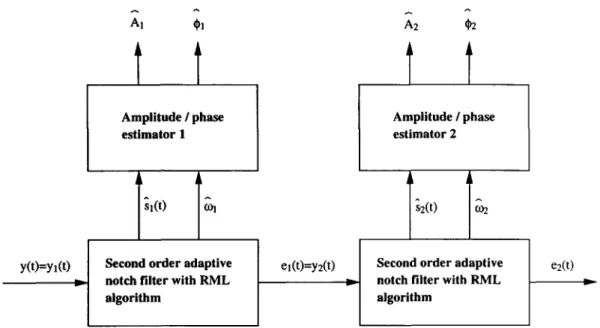
The proposed adaptive notch filter scheme is shown in Fig. 1 for p = 2 case. The major building blocks of the scheme are several second-order adaptive notch filters and amplitude/phase es- timators. The estimation procedures of this scheme can be divided into the following two steps. First, use cascade adaptive notch filters with recursive maximum likelihood (RML) algorithm to extract every sinusoidal signal ~i(t) from input signal y(t)

and to estimate sinusoidal frequencies tbi. Second, each estimated frequencies 03~ and enhanced sine wave gi(t) are sent to the amplitude/phase estimator in order to obtain estimate values of amplitude and phase. Now, let us describe every building block in the following.

2.2. Second-order adaptive notch filter with R M L algorithm

The ith second order notch filter in Fig. 1 is realized by

1 "-~ ai Z - 1 Jr- z - 2

Hi(z) = 1 + raiz-1 + rZz - 2 (2)

which is also used by Nehorai [8] and M'sirdi [5, 6]. Its notch frequency to~ and 3 dB rejection bandwidth B W are given by

o)~ = arccos , (3)

B W = 7t(1 - r). (4)

Let the input and output signals of notch filter Hi(z)

(3)

S.-C. Pei, C.-C. Tseng/Signal Processing 39 (1994) 117 130 119 Amplitude / phase estimator 1 Amplitude / phase estimator 2 y(t)=yl(t)

_I

-I

Til(t) l~

Second order adaptive notch filter with RML algorithm

el(O=y2(t)

l s2(t) T ~

Second order adaptive notch filter with RML algorithm

Fig. 1. Proposed adaptive notch filter scheme for sinusoidal parameter estimation.

e2(t)

parameter a~ is updated by minimizing the cost function

J ( a i , t) = ~ 2 ' - " e i ( n ) . (5)

n = l

Because only second-order notch filter is used here, conventional high order R M L algorithm can be simplified as follows [8].

T h e s e c o n d - o r d e r a d a p t i v e n o t c h f i l t e r w i t h R M L a l g o r i t h m

l n p u t signal: y~(t)

O u t p u t signal: gi(t), el(t)

100 I n i t i a l i z a t i o n : ai(0) = 0, pi(0) = E ( y 2 ( t ) ) q,,( - l ) = ~ , ( o ) = o, y ~ ( - 1) = yi(O) = 0 el( - 1) = el(O) = O, 2 0 ) = 0.9, 2o = 0.99, ro = 0.99, r(1) = 0.8, r~ = 0.99 M a i n loop: (1) ~ i ( t ) = r ( t ) e i ( t - l) -- y i ( t - l) (2) ~hi(t) = ~pi(t) - a,(t - 1 ) r ( t ) ~ i ( t - 1)

- r 2 ( t ) O i ( t - 2)

(3) ~,(t) = y,(t) + y , ( t - 2)

- rZ(t)ei(t - 2) - ai(t - 1)~bi(t)

p i ( t - 1) (4) p,(t) = 2(t) + pi(t - 1)q;~(t) (5) ai(t) = a~(t - 1) + p,(t)~b,(t)~,(t) (6) e~(t) = yi(t) + y , ( t - 2) - r 2 ( t ) e i ( t - 2) - a i ( t ) ~ i ( t ) (7) g,(t) = y ~ ( t ) - e,(t) (8) 2(t + 1) = 2o2(0 + (1 - 20) (9) r(t + 1) = ror(t) + (1 - r o ) r ~ E n d loop.

Note that the frequency estimate tbl can be evalu- ated from Eq. (3). This algorithm takes only 13 multiplications, 14 additions, and 1 division in each iteration, so it is suitable for real time operations. Also, the R M L algorithm is an asymptotically efficient parameter estimation algorithm, so its accuracy is high.

2.3. A m p l i t u d e ~ p h a s e e s t i m a t o r

Assume that the estimated frequency and enhanced sine wave received from adaptive notch

(4)

120 S.-C. Pei, C.-C. Tseng / Signal Processing 39 (1994) 117-130 filter are o5~ and ~(t), respectively. Using both sig-

nals, the following vector equation may be written.

X,O, = C,, ( 6 )

where

Vcos(lrb0 cos(2o31)... Cos(to3i)IT ' X~ = Lsin(lo3i) sin(2cbi) sin(to3i) ] 0 , = [a(t) b(t)] T,

C, = [g,(1) ~,(2) ... ~,(t)] T.

Notice that M'sirdi and Martin use input signal y(t) to construct vector C, [4, 6], i.e.,

C, = [y,(1) y,(2) ... y,(t)] T.

This is a difference between our scheme and theirs. Then the well-known least square solution is given by O, ~--- ( X T X t ) - 1 x T c t = R ( t ) - 1D(t), where R ( t ) = ~ x T x t , D(t) = ~ x T C t .

Moreover, D(t) obeys the following recursive formula:

2

D(t) = t -- 1 D(t -- 1) + ~i(t)[cos(tblt ) sin(cblt)] T.

t 7

(9)

Finally, we propose a simplified RLS algorithm to estimate amplitude and phase as follows:

Simplified R L S Algorithm Input: &i and gi(t) Output: Ai(t) and dpi(t) Initialization: Oi(O)= [0 0] T Main Loop:

(1) O(t) = a,O(t - 1) + 2(1 - at) x gi(t)[cos(o3it) sin(e3it)] T (2) Ai(t) = x/a2(t) + bE(t)

( - b ( t ) ~ (3) ~bi(t)= arctan \ a(t) J End Loop.

Note that at = (t - 1)/t. However, in order to pro- duce a forgetting effect, at may be fixed to be a constant. In the following simulation we choose a, = 0.99.

Thus, the desired amplitude and phase estimates are given by

-4i = ~/a2(t) + b2(t),

. I / -- b(t)'~

q~, = arctan ~ a - ~ j - ) .

Because cosine and sine are orthogonal, it is easy to show that

lim R(t) = I, (7)

t ---~ a 9

where I is the identity matrix. This expression means that when t increases R(t) converges to identity matrix. Thus, computing R(t) is redundant when t is large. It can be omitted. Therefore, the least square solution can be reduced to

Ot = D ( t ) . ( 8 )

2.4. A Comparison to other schemes

(A) Accuracy: In amplitude and phase estimation, we use enhanced signal gi(t) as reference signal, but M'sirdi and Martin use original signal y(t) as reference. Also, signal to noise ratio (SNR) im- provement factor 1-8] is

SNR(g,(t)) 1

- - - ( 1 0 )

SNR(y(t)) 1 - r'

so SNR of ~i(t) is much higher than SNR of y(t) when r approaches unity. As a result, our scheme has better accuracy than M'sirdi's scheme in amplitude and phase estimation.

(B) Complexity: Because M'sirdi uses conventional RLS algorithm to update amplitude and phase, its complexity is proportional to p2. But we

(5)

S.-C. Pei, C.-C. Tseng / Signal Processing 39 (1994) 117-130 121

use simplified RLS algorithm to estimate amplitude and phase, so complexity is only linear with p. Thus, M'sirdi's scheme is less efficient than ours in complexity.

(C) A simple example: In order to compare our

scheme with M'sirdi's scheme more clearly, a Monte Carlo simulation is tested under input data length 1000 and different SNR on the VAX computer. The input signal is

y(t) = A cos 0.2rtt + + A cos 0.3~t + + v(t)

(11) where A is determined in term of SNR. Table 1 and Table 2 summarize the bias and standard deviation

of sinusoidal parameters calculated from 40 inde- pendent trials. F r o m these results it is easy to see that our scheme has better statistical accuracy than M'sirdi's scheme. Moreover, the C P U time of each trial in our scheme is 1.18 s, but the C P U time in M'sirdi's scheme is 1.48 s. Thus, our scheme is su- perior to M'sirdi's scheme in both accuracy and complexity.

3. Error surface analysis of cascade adaptive notch filters

Error surface analysis is very useful for under- standing the convergence of adaptive recursive filters and provides valuable insight [7, 11]. There are

T a b l e 1 Statistical results of M ' s i r d i ' s s c h e m e S N R N /ix A ~1 /i2 L ~2 (dB) Bias × 10 * 3 157.1 0.0846 6 142.4 0.0806 9 1000 114.8 0.0605 12 91.28 0.0425 Standard deviation × 10 4 3 900.8 0.5384 6 897.6 0.3752 9 1000 887.4 0.2672 12 882.1 0.2132 - 230.8 - 205.8 - 194.8 - 189.4 689.8 0.305 245.5 455.7 0.258 174.5 385.8 0.209 - 144.3 335.6 0.201 - 108.1 491.1 1091 0.5612 446.9 349.7 1061 0.3992 336.9 248.8 1053 0.3024 274.8 185.3 1026 0.2063 193.8 T a b l e 2 Statistical results of o u r s c h e m e S N R N / i , f l ~ , /i2 f2 ~2 (dB) Bias × 1 O- 4 3 115.8 0.0846 -- 212.1 -- 517.2 0.305 6 84.99 0.0806 -- 195.3 -- 352.3 0.258 9 1000 -- 82.63 0.0605 -- 179.4 -- 296.1 0.209 12 45.76 0.0425 -- 174.7 - 253.2 0.201 Standard deviation × 1 O- 4 3 797.8 0.5384 429.6 726.4 0.5612 6 777.2 0.3752 303.5 712.7 0.3992 9 1000 768.1 0.2672 213.9 706.9 0.3024 12 750.8 0.2132 164.5 679.9 0.2063 - 161.7 - 133.6 -- 109.8 - 104.9 395.8 299.6 245.5 174.5

(6)

122 S.-C. Pei, C.-C. Tseng/ Signal Processing 39 (1994) 117-130

(a} Input signal y(t)

Output error e(t)

y Adaptive Algorithm

I-

Fig. 2(a). Simultaneous adaption scheme: the cascade second-order adaptive notch filters are updated simultaneously.

0.0 95

1.95 0.05

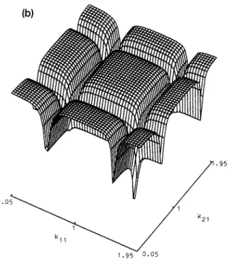
Fig. 2(b). Three-dimensional plot of the mean square error

E(e2(t)) versus the notch filter parameters k~l and k21 for two

sinusoids inputs (p = 2).

two different ways to adjust cascade adaptive notch filter's parameters. O n e is that the filter coefficients are u p d a t e d simultaneously for all stages such as Martin's scheme. The other is that the filter coefficients are u p d a t e d individually in each stage, for

example in M'sirdi's and o u r schemes. Until now, c o m p a r i s o n between these two a d a p t i o n s has n o t been very clear and has n o t a p p e a r e d in the o p e n literature. In this section, we will use the error surface analysis to discuss their difference. T h e results tell us the error surface of simultaneous adaption scheme is multi-dimensional and has local minima. A n d the error surface of individual a d a p t a t i o n is strictly one-dimensional, u n i m o d a l and has g u a r a n t e e d convergence. The one- dimensional solution search space in individual a d a p t i o n is m u c h smaller a n d easier to handle t h a n the multi-dimensional one in simultaneous adaption.

3.1. S i m u l t a n e o u s adaptive s c h e m e

Fig. 2(a) shows the system that the cascade adaptive notch filters are u p d a t e d simultaneously. The input signal consists of p sinusoids in addition to white noise, as expressed in Eq. (1). M a r t i n has chosen a low coefficient sensitivity b i q u a d as desired s e c o n d - o r d e r n o t c h filter, i.e.

2 - ki2 1 - - 2(2-kiz-k21)Z2-ki2 1 ql- Z - z

Hi(z) - 2 1 - (2 - ki2 - k'Z,1)z -1 + (1 - klz)z -2

(12)

where k i 2 = 1 - r 2 a n d kil = 2 x / l - ( k 1 2 / 2 ) sin(~o~/2) if r is pole radius a n d ~o~ is n o t c h

(7)

S.-C. Pei, C.-C. Tseng / Signal Processing 39 (1994) 117-130 123

to}

_.95

J

,,.,.J 16 r

f

1 k21 --.._~ 16

I

/ ,

\

I IIII

t

!

I

o-°~

I 1.95 0.0 kl I

Fig. 2(c). Error surface contour plot and the trajectories of three simulations initialized at the points (k 11, k21 ) = (a) ( 1.2, 1.2), (b) (1.0, 1.0) and (c) (1.8, 0.8) respectively.

frequency. The objective of the simultaneous ad- aptation algorithm is to adjust the k~l's such that the output mean square error

E(e2(t))

is minimized. During adaption, 3 dB rejection bandwidth is kept constant by choosing a fixed value for kg2's. It is easy to show that the mean square error is

E(eZ(t)) = ~ A~

~-IH(eJ~")l 2 +

a2 ~

In(z)l 2dz,

I13)

where c is a counterclockwise unit circle contour, and

H(z) = I]f= xHi(z).

The first term of Eq. (13) is closed-form formula, we can calculate it exactly by computer. However, the second term is difficult to simplify by the Cauchy's residue theorem, so we use numerical integration, such as Trapezoid rule, to compute its approximate value through the following equation:

(8)

124 S.-C. Pei, C.-C. Tseng / Signal Processing 39 (1994) 117-130

Now, we consider an example with the input signal

a s

y(t)

= x/26cos(0.2rct) + x / ~ c o s

.6r:t + ~ + v(t).

(15)

M'sirdi's scheme and ours is

Hi(z)

which is expressed in Eq. (2). In each stage, the objective of the adaptive algorithm is to adjust al such that the mean square error

E(e{(t))

at each stage is minimized. F o r the first stage, it is easy to show that

A 3D plot of the mean square error

E(e2(t))

versus the two notch parameters k~l, k2~ is depicted in Fig. 2(b) for r = 0.95. F r o m the plot, we observe that the local minima are at four ditches kll = 0.603, kll = 1.579, k 2 1 = 0.603, and k 2 1 ~- 1.579. When the notch parameters are up-

dated and converge to one of these four ditches, the cascade adaptive notch filter can only eliminate one sinusoid, while the other will still exist. Further- more, we observe that there are two minima at deep troughs (kll,k21) = (0.603, 1.579) and (1.579, 0.603). When the notch parameters are adjusted and converge to one of two troughs, the cascade adaptive notch filter can eliminate two sinusoids successfully. In order to understand the convergence behavior of Martin's algorithm, we use his algorithm to adjust the parameters of notch filter. These examples are illustrated in Fig. 2(c). Initial points of the three examples are (kll, k12)= (1.2, 1.2), (1.0, 1.0), and (1.8, 0.8). In each example, the parameters are adjusted by 1000 iterations. As a result, we find that the trajectory initialized at (1.0, 1.0) converges to (0.603, 0.603). Even though it is updated 4000 iterations, it still stays there. This situation means that the two notch stages both converge to the same sinusoid's frequency which is not the desired minimum solution. F r o m the above description, we know that there are two local mini- mums at (0.603, 0.603) and (1.579, 1.579). Therefore, mean square error surface of cascade adaptive notch filter which is updated simultaneously is multimodal, so a judicious choice of the initial parameters is important.

3.2. Individual adaptive scheme

Fig. 3(a) shows the system that cascade adaptive notch filters are updated individually. The input signal is still p sinusoids in an additive white noise as above. The second-order notch filter used in

E(e~(t)) = ~ A{

_{i=1 2 - [ H 1 (eJ°'i)12}

(16)

Fig. 3(a) shows the error surface of

E(eZ(t))

versus al when the input signal is

(17)

It is interesting to see that the error surface is one-dimensional and has two distinct minima asso- ciated with each frequencies, so the first stage will converge to one of the two sinusoid's frequencies. Because the second order notch filter's frequency response is unity gain and zero phase everywhere except near the notch frequency, the other sinusoid signal and noise pass through the filter

Ha(z)

almost undistortedly. Thus the mean square output error of the second stage is

E(eZ(t)) =

v _A~2 _{(r E} _dz

i=l.i+-k

2 [H2(eJ°i)12 + ~ j [H2(z)12z

(18)

where k is the sinusoid removed by the first stage. The whole situation of the second stage is the same as the first stage, and one of the other sinusoids will be eliminated by the second stage. Repeat this process until all of the sinusoids are eliminated individually in each stage. Fig. 3(c) shows the learning curves of the parameters ai, i - - 1, 2 in the two stages when the input

y(t)

is expressed in Eq. (17). This figure reveals that two sinusoidal frequencies can be estimated correctly and quickly by cascading notch filters. Therefore, the error surface of second order notch filter which is updated individually is unimodal and has no local minima.

(9)

S.-C. Pei, C.-C. Tseng/Signal Processing 39 (1994) 117 130 125 (a) Input signal y(t) ~ [

I

HI(Z)

Adaptive F

Algorithm

el(t)

li

H2(z)

Adaptive

Algorithm

e2(t)

Adaptive

Algorithm

Output error ep(t)=e(t)

J-

° I

~

) 2 4 £3 I , - 2 . 0 - 1 . 2

V

, I , , , , I , , , , 0 . 4 1 . 2 2 . 0 F oh k |.. 1- - 2 ( 2 ) I "L/ ...

Z

its!!! ( 1 ) , ~ , I , , , , , ~ [ , ~ , L I i i I i I , , , L I , ~ , , - 0 • 4 2 0 0 4 0 0 6 0 0 8 0 0 1 0 0 0 a, i t e r a t i o n

Fig. 3. (a) Individual adaption scheme: the cascade second order adaptive notch filters are updated individually. (b) The error surface plot of the mean square error E(e2(t)) versus the notch filter parameter al for two sinusoidal inputs. (c) The learning curves of the two

stage notch filter parameters al and a2 for two input sinusoids. [(1) solid line: first stage, (2) dot line: second stage]

4. Computer simulations

S o m e e x p e r i m e n t s are run on the VAX 11/780 c o m p u t e r to test the p r o p o s e d scheme for sinusoidal p a r a m e t e r e s t i m a t i o n a n d the t r a c k i n g p e r f o r m a n c e with R M L algorithm.

Example

1. (Tracking stationary input). In the

example, the input signal is

(19)

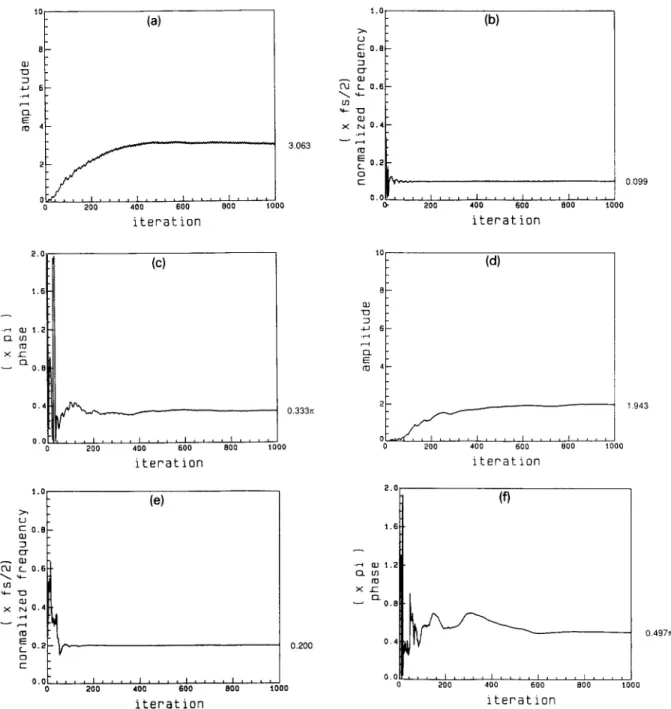
Fig. 4 shows the learning curves of each sinusoidal p a r a m e t e r s of p r o p o s e d scheme respectively. As

a result, b o t h stages converge to the correct solution as expected.

Example

2. (Tracking non-stationary input). In the

example, we will study the tracking b e h a v i o r of p r o p o s e d scheme for the n o n - s t a t i o n a r y input. We m a k e s o m e c o m p a r i s o n s with M a r t i n ' s simultaneous a d a p t i o n scheme in a various condition. T h e scenario of the e x p e r i m e n t is similar to the E x a m - ples 1 - 4 in Ref. [3]. F o u r different cases are inw.st- igated as follows:

(A) Two sinusoids are not close to each other in frequency. Let the input signal be

y(t) =

{

x / ~ c o s ( 0 . 3 n t ) + x/~cos(0.27zt) + v(t) if t ~< 400,

(10)

126 S.-C. Pei, C.-C. Tseng/ Signal Processing 39 (1994) 117 130 QJ 4-J (D_ E

(a)

, , , I . . . . 1 , , , , I i i , , I , , , , 2 0 0 4 0 0 E 0 O B O O t 0 0 0 iteration 3.063 cu u~ × t.(] rJ ¢ - 0 . ~ 0J ET 0J L 0 . E 0J N 0 . t nJ Q t- o.( 0-

(b)

2 0 0 4 0 0 6 0 0 8 0 0 t O O 0 i t e r a t i o n 0.099 n

×~

rn 2 . 0

(c)

t . 6 1 . 2 0 . B

i:

....

. . . 0 2 0 0 4 0 0 6 0 0 8 0 0 i t e r a t i o n 0.333= t 0 0 0 t 0 B

~ 6

O. E (~ 4 ¸

(d)

1 9 4 3 , , S ~ I , , , , I . . . . I . . . . I , , , , 2 0 0 4 0 0 6 0 0 8 0 0 t 0 0 0 i t e r a t i o n u c 0J ZI O" 03 CM c_. (/3 v,_ "t~ oJ x N r0 0 C t . o o . e 0 , 6 0 . 4 0 . 2

o,%

(e)

i t i , I . . . . I . . . . I , , , , I , , , , 2 0 0 4 0 0 6 0 0 8 0 0 t O 0 0 i t e r a t i o n 0 . 2 0 0

2"~'

I,.6

(f)

• ~ 0A t.2 x r- , , , , , i i , , I i , , i r i , , r 0 2 0 0 4 0 0 6 0 0 8 0 0 1000 iteration

Fig. 4. (a) T h e l e a r n i n g c u r v e of the a m p l i t u d e in the first stage. (b) T h e l e a r n i n g c u r v e of the frequency in the first stage. (c) T h e l e a r n i n g c u r v e of the p h a s e in the first stage. (d) T h e l e a r n i n g c u r v e of the a m p l i t u d e in the s e c o n d stage. (e) T h e l e a r n i n g c u r v e of the frequency in the s e c o n d stage. (f) T h e l e a r n i n g c u r v e of the p h a s e in the s e c o n d stage.

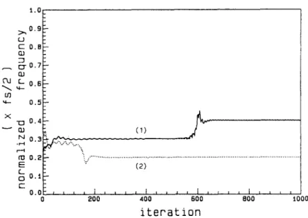
After 400 samples, one sinusoid's normalized fre- quency is changed from 0.3 to 0.4 suddenly. Fig. 5 shows the learning curve of frequencies of 2 stage second-order system. The first stage converges to the

sinusoid with frequency 0.3 in the beginning and then tracks the sinusoid at 0.4 quickly. The second stage always deletes the sinusoid at 0.2 without change.

(11)

S.-C. Pei, C.-C. Tseng/Signal Processing 39 (1994) 117 130 127 1.0 > O . g u

~

O.B g O . 7 O3 CU f - - o . f i U'J ,4- 0 . 5 X S - r - ' l ro E c'- 0 . 4 0 . 3 0 . 2 0 . t 0 . 0 ~ ~ ~ ~ i 0 2 0 0 (1) _ ~ ' ~ (2) , , I , , , , 1 , , , , I , , , , 4 0 0 6 0 0 8 0 0 t000 iteration

Fig. 5. The learning curves of frequencies of 2 stage second-order systems for two input step changed sinusoids which are separated in frequencies. [(1) solid line: first stage, (2) dot line: second stage]

(B) (Two sinusoids are close to each other in fre-

quency.) The input signal is

y(t) =

{

x/~cos(0.3nt) + x~6cos(0.Z5r~t) + v(t) if t <<. 400 x/26cos(0.4rtt) + x~cos(0.25rtt) + v(t) if t >400. Two sinusoids in this example are closely spaced at normalized frequencies of 0.25 and 0.3. Refering to Fig. 6(a), the first stage converges to 0.3 and the second stage converges to 0.25 in the beginning. Also, a 'ripple' effect occurs in the first stage because of the influence of nearby sinusoid at 0.25. When the input frequency at 0.3 is step changed to 0.4 after 400 samples, the first stage starts tracking and switches converged frequency from 0.3 to 0.25. This is because the frequency at 0.3 is much closer to 0.25 than the frequency at 0.4. It will force the second stage to change converged frequency from 0.25 to 0.4. This means that the first stage has higher priority than the second one during the adaption process. In addition, the same situation is tested for Martin's simultaneous adaption scheme. Refering to Fig. 6(b), the result is interesting and quite different from Fig. 6(a). The first stage changes converged frequency from 0.3 to the dis-

tant frequency at 0.4 instead of the close one at 0.25, and the second stage always converge at 0.25 without change. This is because the simultaneous adaption algorithm minimizes the final output mean square error. The advantages of Martin's scheme are that it has no 'ripple' effect and it has global tracking mechanism. However, large complexity and heavy computation are required for Martin's scheme. Simplicity and comparable performance can be obtained by our individual adaption scheme.

(C) (Two sinusoids are close in frequency with

large power difference.) The input signal is

y(t)

= 2w/~0 cos(0.24rtt) + x~cos(0.28rtt)+

v(t).

(20)

The input consists of two closely spaced sinusoids with SNR of 20 and 0 dB at frequencies 0.24 and 0.28 respectively. Refering to Fig. 7, after the first stage converges to the large power sinusoid at 0.24, the second stage quickly tracks the sinusoid with the smaller power. No ripple effect is seen in this case due to the very little effect with the smaller power sinusoid has.

(12)

128 S.-C. Pei, C.-C. Tseng/Signal Processing 39 (1994) 117 130 1 . 0 0.9 :>,, r..J c - 0 . 8 Z3 C T 0 . 7 ('%1 f'-- 0 . 6 0.5 x ~ o.4i a 0 . 3 ° r-'-¢ r - - i ro 0.2 E ~oo.'1 c" 0.11 t . 0 :>.O.9 rJ r- 0 . 8 ~1~" 0 . 7 Ill t"kl L O . 6 0.5 X -Ej 0.4 N 0.3 - r ~ . r " ' ( t o o . 2 E ~ 0 . ~ . r- 0.0

(a)

(I) i (2) | I I I I I i 200 400 600 800 t000 iteration

(b)

(2) 2 0 0 400 600 800 1 0 0 0 iteration

Fig. 6. (a) The learning curves of frequencies of 2 stage second-order systems for two input step changed sinusoids which are closely spaced in frequencies. [Individual adaption scheme: (1) solid line: first stage, (2) dot line: second stage.] (b) The learning curves of frequencies of 2 stage second-order systems for two input step changed sinusoids which are closely spaced in frequencies. [Simultaneous adaption scheme: (1) solid line: first stage, (2) dot line: second stage.]

(D)

(Sixth-order adaptive notch filter system.)

The input signal is

Refering to Fig. 8, the first stage tracks the time- varying sinusoid switched from 0.3 to 0.25 instead

)'x/~cos(0.257tt) + x / ~ c o s ( 0 . 3 n t ) + x / ~ c o s ( 0 . 5 n t ) +

v(t)

if t ~< 400

(13)

S.-C. Pei, C.-C. Tseng / Signal Processing 39 (1994) 117-130 129 t . 0 0 . 9 r...J E Z O . 8 0..) 23 0"0.7 (33 OJ L O . 6 CO 0 . 5 X - E D 0 . 4 N 0 . 3 - e,.-s r-t m 0 . 2

E

O 0 . 1 c" 0.0 '--. ( 2 ) i ..~ ... i ... (1) , , , I , , , , I , , , I , , , , I , , , , 2 0 0 4 0 0 6 0 0 8 0 0 ~ . 0 0 0 i t e r a t i o n

Fig. 7. The learning curves of frequencies of 2 stage second-order systems for two input sinusoids which are closely spaced in frequencies with large power difference.

1.0 2 > 0 . 9 _ u c- 0.8 O - 0 . 7 £ ' - 0 . 6 0"] ,4-- 0 . 5 X ] 2 ] 0 . 4 ~ a3 N 0 . 3 .r--I r ~ rO 0 . 2 E L O 0.1 C 0 . 0 0

(~

t (I) -

L.j-.

. . .

~'/

200 400 600 800 ~000 iteration

Fig. 8. The learning curves of frequencies of 3 stage second-order systems for three input step changed sinusoids which are separated in frequencies, [(1) solid line: first stage, (2) dot line: second stage, (3) dash line: third stage.]

of 0.4. This is because the frequency at 0.3 is much- closer to 0.25 than the frequency 0.4. This forces the third stage to j u m p from 0.25 to 0.4. A similar situation happened also in case (B) as above. The second stage always stays at the distant sinusoid at 0.5 without change.

5. Conclusion

In this paper, we have proposed a cascade adap- tive notch filter scheme for sinusoidal parameter estimation and tracking. Our scheme uses en- hanced signal as reference of amplitude/phase

(14)

130 S.-C. Pei, C.-C. Tseng/ Signal Processing 39 (1994) 117-130

estimator. This improves the accuracy of amplitude and phase estimation. Also, the RLS algorithm is simplified to adjust the amplitude and phase. Error surface analysis indicates that our scheme is unimodal and results in guaranted convergence.

References

[1] B. Friedlander and J.O. Smith, "Analysis and performance evaluations of an adaptive notch filter", IEEE Trans. In-

form. Theory, Vol. IT-30, March 1984, pp. 280-295.

1-2] D.R. Hush, N. Ahmed, R. David and S.D. Sterns, "An adaptive IIR structure for sinusoidal enhancement, fre- quency estimation and detection", IEEE Trans. Acoust.

Speech Signal Process., Vol. ASSP-34, December 1986, pp.

1380-1390.

[3] T. Kwan and K. Martin, "Adaptive detection and enhancement of multiple sinusoids using a cascade IIR fil- ter", IEEE Trans. Circuits and Systems, Vol. CAS-36, July 1989, pp. 937-947.

[4] K. Martin, "The isolation of undistorted sinusoids in real time", IEEE Internat. Syrup. on Circuit and Systems, Port- land, USA, May 1989, pp. 2112 2115.

[5] N.K. M'sirdi and H.A. Tjokronegoro, "Cascade adaptive notch filters: an RML estimation algorithm", European

Signal Process. Conf., Grenoble, France, September 1988,

pp. 1408-1412.

1-6] N.K. M'sirdi, H.A. Tjokronegoro and I.D. Landau, "An RML algorithm for retrieval of sinusoids with cascaded notch filter", 1988 lnternat. Conf. Acoust. Speech Signal

Process., New York, USA, April 1988, pp. 2484-2487.

[7] M. Nayeri and W.K. Jenkins, "Alternate realizations to adaptive IIR filters and properties of their performance surfaces", IEEE Trans. on Circuits and Systems, Vol. CAS- 36, April 1989, pp. 485-496.

[8] A. Nehorai, "A minimal parameter adaptive notch filter with constrained poles and zeros", IEEE Trans. Acoust.

Speech Signal Process., Vol. ASSP-33, August 1985, pp.

983 996.

1-9] T.S. Ng, "Some aspects of an adaptive digital notch filter with constrained poles and zeros", 1EEE Trans. Acoust.

Speech Signal Process., Vol. ASSP-35, February 1987, pp.

158 161.

[10] D.V.B. Rag and S.Y. Kung, "Adaptive notch filtering for the retrieval of sinusoids in noise", IEEE Trans. Acoust.

Speech Signal Process., Vol. ASSP-32, August 1984, pp.

791-802.

1-11] S.D. Sterns, "Error surface of recursive adaptive filters",

IEEE Trans. on Acoust. Speech Signal Process., Vol.