ADAPTIVE-CONTROL OF A CLASS OF NONLINEAR DISCRETE-TIME-SYSTEMS USING NEURAL NETWORKS

JEE TRANSACTIONS ON AUTOMATIC CONTROL, VOL. 40, NO. 5, MAY 1995 791

Adaptive Control

of

a Class

of Nonlinear

Discrete-Time Systems

Using

Neural Networks

Fu-Chuang Chen, Member, ZEEE,

and

Hassan

K.

K h a , Fellow, ZEEE,

Abstracr-Layered neural networks are used in a nonlinear

self-toning adaptive control problem. The plant is an unknown feedback-hearimble discrete-time system, q ” t e d by an input-ut model. To derive the linearizing-stabilizing feedback control, a @ossiMy n o “ a l ) state-space model of the plant

is obtriwd. This model is used to define the zero dynamics, whieb am rrarsnaaed to be stabk, i.e., the sptm is 81wllllbd to

be phase. A I k a r M n g feedback contdisderived in

terms of some unknown nonlinear fimctions. A layered neural network is used to model the unknown system and generate the feedback control. Based on the error between the plant output and the modd output, the weights of the neural network are updated. A local convergeace result is given. The result says that, for any bounded initial conditions of the plant, if the neural network model conta€ns enough number of nonlinear bidden neurons and if the initial guess of the network weights

is sufficiently close to the correct weights, then the tracking error between the plant output and the reference command will

converge to a b o d e d ball, whose size is determined by a dead- zone nonlinearity. Computer simulations verify the theoretical mdt.

I. INTRODUCTION

DAPTIVE control of linear systems has been an active

A

research area in the past two decades. It is only recently that issues related to adaptive control of feedback-linearkable nonlinear systems are addressed, e.g., [ll, [31, and 141. An important assumption in previous work on nonlinear adaptive control is the h e a r dependence on the unknown parameters, i.e., the unknown nonlinear functions in the plant have the form

n

f(.)

= O i f i ( . ) (1) i=l

where fi’s are known functions. The linear parameterization

(1) is also used in the recent work [2] on applying Gaussian networks to an adaptive control problem.

Multilayer neural networks can be considered as general tools for modeling nonlinear functions. The network comprises fixed (sigmoid-type) nonlinearities and adjustable weights which appear nonlinearly. Learning algorithms are used to Manuscript received October 8, 1991; revised May 7, 1993. Recommended by Past Associate Editor, A. Arapstathis. This work was supported in part by National Science Foundation Grants ECS-8912827 and ECS-9121501 and National Science Council of the Republic of China Grant NSC-81-0404-E-

009-005.

F.-C. Chen is with the Department of Control Engineering, National Chiao l h g University, Hsinchu, Taiwan R.O.C.

H. K. Khalil is with the Department of Electrical Engineering, Michigan State University, East Lansing, MI 48824 USA.

EEE Log Number 9409416.

adjust the weights so as to reduce the modeling error. With the introduction of the back-propagation learning algorithm by Rumelhart et al. [5] in 1986, the multilayer neural network has become a popular architecture for practical applications in many areas, including system identi6don and control, signal processing, and pattern classification. some of the actihties in identikation and control problems have been reported in [6].

The idea of applying multilayer neural networks to adap- tive control of feedback-linearizable discrete-time systems appeared in [7] and [8]. In [13] we presented a convergence result for adaptive regulation using multilayer neural networks. Many restrictive assumptions, however, were made in [13]. As we worked on relaxing these assumptions, it became clear that the updating rule used in [ 131 would not be adequate.

To

cope with this problem, we incorporate a dead-zone nonlinearity in the weight updating rule, adapted from Kreissehneier and Anderson [14]. The control algorithm, the modified updating rule, and a convergence theorem are given in Section III.

The control scheme and the convergence result presented in this paper are applicable to nonlinear discrete-time systems with a general relative degree. For a system with a relative degree higher than one, the cancellation control cannot be dehed explicitly because of a causality problem, i.e., current controls depend on future outputs. A similar problem appears in the linear case and has been discussed in [15] and [16]. In Section II, we generalize the results of [15] and [16] to the nonlinear case. We also define the zero dynamics and the minimum phase property of a nonlinear system. Minimum phase is one of the conditions of our convergence theorem. Finally, simulation results are given in Section IV.

n.

LINEARJZING FEEDBACK CONTROL

We are interested in the single-inpdsingle-output nonlinear discrete-time system

where fo and go are smooth (i.e., infinitely differentiable) functions of

m

5

n, y is the output, U is the input, d is the relative degree of

the system, and go is bounded away from zero. The arguments of fo and go are real variables.

792 IEEE TRANSACTIONS ON AUTOMATIC CONTROL, VOt. 40, NO. 5, MAY 1995

There are two difficulties when we try to linearize system (2) via feedback. First, the control law cannot simply be

with r(k) being the reference command, because this control is noncausal when d

>

1. Second, since fo and go depend on past inputs, the system may become internally unstable after the feedback control, if it exists, cancels the plant dynamics. These two issues are weIl known for linear discrete-time systems

[15], [16]. The purpose of this section is to resolve these difficulties for the nonlinear system (2).

To define the zero dynamics and to facilitate developing the conve ence proof, the inpudoutput form (2) of the system is as the current output and all past inputs and outputs up to the

most delayed input or output on the right-hand side of (2), i.e., conve

f

ed into a state-space form. We select the state variables

Zi(k) = Yk-n+i, for i = 1,2, * * ' ,TI,

Zn+i(k)=Uk-m-d+i, for i = 1 , 2 , * * * , m + d - l . Let x(k) be the state vector. A state-space model of (2) is constructed accordingly as zi(k+l)=zi+l(k), for i = 1 , 2 , - . . , n - l zn(k

+

1) = fO[X(k)]

+

90[X(k>lZn+m+l(k) Zn+i(k

+

1) = Zn+i+l(k), for i = l , 2 , . . . , m + d - 2 zn+m+d-l(k

+

1) =uk Y(k) =zn(k). (3)

When d = 1, the second equation of (3) is

zn(k

+

1) = fO[X(k)l+ 90[X(k)I%

Hence, the input-output map of the system can be linearized by a causal state feedback control that cancels the nonlinearity. When d

>

1, we need to do more work to be able to cancel the nonlinearity by a causal state feedback control. The trick is to represent future plant outputs in terms of elements of x(k). Notice that zn(k

+

1) = 2/k+l. Then

zn(k+2) = fo[x(k+ I)] +go[x(~+l)]z,+m+1(~+1). (4) Replacing x(k

+

1) in (4) by the right-hand side of (3), we have'

zn(k

+

2) = fl[X(k)]

+

91[X(k)]zn+m+2(k). By applying the same technique recursively, one gets

zn(k

+

3) = f2[x(k)l

+

g2[x(k)Izn+m+3(k),

Zn(k

+

d - 1)

'Notice that fo and go depend only on 21 to .,+%, Therefore, substitution the argument of fo and go. The fd_Z[X(k)]

+

gd-2[x(k)]sn+m+d-l(k). of x ( k

+

1) from (3) does not bring U k

new functions f i and g1 depend on 11 to 1,+,+1.

Consider the state transformation

z(k) =

It can be shown that the inverse of

(3,

i.e., x = T-l(z), exists provided go(x), gl(x),

,

gd-z(x) are bounded away from a m over the domain of interest. After application of the transformation (S), (3) becomes Zli(k

+

1) = Zl,i+l(k), Zl,m+d-l(k

+

1) =fd-l[x(k)J for i = 1,2,... , n + d - 2

+

gd-l[X(k)]Zn+m+d-l(k

+

1) = fd-1(T-1[Z(41)

+

Qd-1 {T-l [Z(k)]}U& = F [ z ( k ) ]

+

G[z(k)l~k z24k

+

1) = ZZ,i+l(k), for i = 1 , 2 , . . - , m - 1 Y(k) = Zln(k). (6)

when d = 1, the state vector z does not contain the compo- nents zli for i

>

n, and the state equation in the z coordinates takes the form (6) except that zzm(k

+

1) = Uk. To deal with

the cases d = 1 and d

>

1 simultaneously we rewrite (6) as ZlZ(k

+

1) =Zl,i+l(k), for i = 1 , 2 , - . . , n + d - 2 Zl,n+d-l(k

+

1) = F [ z ( k ) ]

+

G[z(k)]u& Z 2 i ( k

+

1) = ZZ,i+l(k), for i = 1,2,..- , m - 1 (7) where Uk-d+l = Uk when d = 1, while for d

>

1 we have

The feedback control

(9)

linearizes the input-output map of the system and r(k) appears as desired output d steps later. This transformation procedure is illustrated by the following example.

793

CHEN AND MAL& ADAPTIVE CONTROL OF DISCRETE-TIME SYSlI34S

I Eranrple: For n = m = d = 2, the system takes the form

Replace the Yk+l term in (11) by the right-hand side of (10)

to obtain

Yk+2 = fO[Yk 7 fO(Yk-1, Y k , Uk-3, uk-2)

The two functions f1 and g 1 depend on past inputs and outputs;

thus, the control Uk can be defined in terms of

f~

and 9 1 . U

Following Monaco and Norman-Cyrot [ 171, the zero , dy-

namics are defined as the unobservable dynamics when the control (9) is used, namely

Since the dynamics associated with z l i , for i

=

1,

-

.

,

n

-

1 ,

~ t e always stable, we define the system to be mini” phase if

(13) has an asymptotically stable equilibrium point C = [c,c, ,cl’. Equation (12) defines the internal dynamics of the system when the reference command r(k) and the plant output yk are constrained to be identically zero. Since zli, for i = 1 , 2 , . . . ,n

+

d

-

1 are either forward or backward shifts of ark, constraining gk to be identically zero implies that zli =

0, for i = 1,2,

,

n

+

d - 1 and the closed-loop equation reduces to (13). Note that (13) is the same equation that is obtained from (2) by constraining gk to be identically zero.

m.

ADAPTIVE CONTROL USING NEURAL NETWORKS Consider now the case when n, m, and d are known, but the nonlinear functions F ( 0 ) and G ( o ) in (7) are unknown. We use multilayer neural networks to model the unknown nonlin- earities. It has been shown by Funahashi [lo], Cybenko [ll], Hornik et al. [12], and Hecht-Nielson [9], using different tech- niques, that multilayer neural networks can approximate any “well-behaved” nonlinear function to any desired accuracy. The statement of Funahashi’s theorem [lo] is quoted here.

Theorem: Let +(z) be a nonconstant, bounded, and mono- tonically increasing continuous function. Let

S

be a compact subset of Rn and f ( z l , + . - ,z,,) be a real valued continu- ous function on S. Then for any E

>

0, there exists an

integer N and real constants c+ei(i = l , . . . ,N),wij(i =

1 , e - s , N , j = 1 , e . e ,n) Such that

N / n \

satisfies max,Es-lf(zl,.-. ,zn) - f ( z : , , . . - ,zn)l

<

E . The network f in (14) contains one nonlinear hidden layer. Similar results for neural networks with more than one hidden layer can be derived from the theorem above or be shown from scratch [lo]. Funahashi’s theorem, however, provides only an “existence” result. The network size N and the network parameters 48, W;~S, 0:s are not determined by the theorem.

To proceed with our development, we state our assumptions on the plant.

Assumption I: go(x), e

,

g d - l ( x ) are bounded away from

zero over S, a compact subset of P+m+d-l, that is

(15)

vx E

s.

Assumption 2 (The Minimum Phase Assumption): The

19i(X)l

1

b

>

0,

change of variables e2; = z2i - c transforms (13) into

e z i ( k - t l ) = e z , i + l ( k ) , for i = l , 2 , - . . , m - 1

in some ball BPa C Rm. The existence of a Lyapunov function satisfying these condition is guaranteed by a converse Lyapunov theorem [ 131.

Rewrite the plant in an input-output form as

Yk+d = f d - l [ x ( k ) l + gd-l[x@)IUk. (18)

Recall from (6) that f d - l ( x ) = F(z) and g d - l ( x ) = G(a).

Plant (18) is modeled by the neural network

(19) The functions fd- 1 (-

,

.) and J d - 1 (

-

,

-) depend on the structure of +e neural network and the number of neurons. For example, if fd-1 ( e , .) and j d - ~ ( . , a ) are three-layer neural networks

with p and q hidden neurons, respectively, then they can be expressed as

&+d = j d - l [ X ( k ) , w]

+

4 d - l [ X ( k ) , VI%

P

f d - l [ x ( k ) , w 1 = wiH i=l

I94 IEEE TRANSACTIONS ON AUTOMATIC CONTROL, VOL. 40, NO. 5, MAY 1995

and

m+n+d-1

i=l

According to Funahashi's theorem, the function H in (20) and (21) has to be continuous, bounded, nonconstant, and monotonically increasing. We require, in addition, that H be differentiable. The differentiability of H is needed in our updating rule and convergence analysis. Throughout this research, we have used the hyperbolic tangent function

in computer simulations, but other functions having the fore- going properties couId be used.

Assumption 3: Given a positive constant E and a compact

set S C Rn+m+d-l, there exist coefficients w and v such that

fd- 1 anti j d - 1 approximate the continuous functions fd- 1 and gd-1, with accuracy E over S, that is

3 w, v s.t. max l f d - l ( x ,

w)

-

f d - l ( x ) I

5

E and

m m I 6 d - l ( x , v ) - g d - l ( x ) (

5

€ 7

vx E

s.

(22)

This assumption is justified by the approximation results of 191-[12]. In our work we assume that the structure of the net- work and the number of neurons have been already specified, and (22) holds for the plant under consideration, but we do not assume that we know the weights w and v for which (22) is satisfied. Let w(k) and v(k) denote the estimates of w and v at time

k.

Then the control uk can be defined as the following.

Control Law:

where r ( k ) is the reference command.

The control U & is applied to both the plant and the neural

network model. The network weights are updated according to the error between the plant and model outputs. To better define the error, rewrite (18) and (19) as

Y&+l = fd-1 [x(k

-

d

+

I)]

+

gd-1 [x(k

-

d

+

l)]U&-d+l (24)

and

$&+l = fd-l[X(k - d

+

I), wl

+

j d - l [ x ( k - d

+

1)1V]u&-d+l. (25) The estimated plant output is

Yi+1 = f d - I [ x ( k

-

d + 1),w(k)]

+

6d--l[X(k - d

+

11, v ( k ) ] u & - d + l - ₍₂₆₎

The error e;+1 is defined as

.;+I = Y;+1 - Y k + l (27)

which will be used in the weight updating rule to be described next.

Let 8 =

[TI.

The problem of adjusting the estimate

8 ( k ) on-line is a typical problem in adaptive conFo1. The new element here is the fact that the functions fd-1 and j d - 1 depend nonlinearly on the parameter 8. In the adaptive

control of linear systems, or even linearizable continuous-time systems [3], the corresponding functions depend linearly on the unknown parameter 8. This nonlinear dependence on 8 is the main challenge in the current problem. In a previous work [13], we studied an updating rule of the form

where

and

~k = 1

+

J i - d + l J k - d + l .

The variable is the output of a multilayer neural network. Hence, the Jacobian matrix Jk-d+l can be calculated using the

routines of the backpropagation algorithm [5]. We were able to prove an asymptotic regulation result, under some restrictive assumptions, like assuming that the nonlinearty fd-1 vanishes

at the origin and that fd-1 and gd-1 can be modeled perfectly by neural networks, that is, 6 = 0 in (22). As we tried to

relax these restrictions and work on the tracking problem, it became clear that the learning rule (28) would be inadequate. The source of the problem is partly from model uncertainties in the stability analysis. Related problems have been extensively studied in the literature on robust adaptive control [ 181, where a number of modifications of the simple gradient algorithm have been proposed to cope with robustness problems. We are going to employ a dead-zone algorithm for updating the weights which has been adapted from [14]. At each time step, if the error between the plant output and the model output is larger than a certain threshold, the weights are updated. Otherwise, the weights are not changed. To implement this, the error e;+, defined in (27) is applied as input to a dead-zone function D(e), defined by

if

1.1

5

do

D(e) =

("

e - do if e

>

6

(29) e + d o if e < - & .

The output of the dead-zone function is used in the updating rule.

Updating Rule:

CHEN AND MALIL: ADAPTIVE CONTROL OF DISCRETE-TIME SYSTEMS 795

7"heoremI: Suppose Ir(k)l

5

dl for all k

2

0. Given any constant p

>

0 and any s m a l l constant do

>

0, there exist positive constants p 1 = p 1 ( p , dl), p 2 = p2(p, dl), E* =

~ * ( p , do, dl), and 6* = S*(p,

do,

dl) such that if Assumptions 1 and 3 are satisfied on 5'II B,, with E

<

E * , Assumption 2

is satisfied on Bpa, I ~ ( 0 ) l

5

p, and le(0)I

I

6

<

6*, then will be monotonically nonincreasing, and

IQ

(k

+

will converge to zero.

2) The tracking error between the plant output and the reference command will converge to a ball of radius do centered at the origin.

Pro08

Step I : The dynamics associated with zl [see (7)] are

z ~ ; ( k + l ) = z l , i + ~ ( k ) , for i = l , 2 , . . . , n + d - 2 z l , n + d - l ( k ) = F [ z ( k ) ]

+

G[z(k)]uk. (32)

The last equation can be rewritten as

~ l , n + d - l ( k

+

1) =J'[z(k)]

+

G[z(k)]~k = P [ z ( k ) , w]

+

G[Z(k),V]Uk

+

(J'[z(k)l

-

@Iz(Js), WI

+

{G[z(k)l - G [ z ( k ) , VI)Uk)l =fi[2@),wl+ G[z(k),V].k

+

{.}1 (33) where @[z(k), w] = fd-l{T-'[z(k)], w } and G[z(k),v] = & ~ 1 { T - ' [ z ( k ) ] , v } . Plugging Uk into (331, we have

ZlpI+d-l(k

+

1) = P [ z ( k ) , w]

+

G[z(k),v] = @ ( I C ) , w]

+

G [ z ( k ) , VI - f i [ z ( k ) , w]

+

r ( k )

+

G [ z ( k ) , VI Define eli(k) = w ( k ) - r ( k - n - d

+

i). (35)

Then (32) can be represented in new state variables el as

With the transformation

the dynamics associated with 2 2 are transformed into

Thus, (36) and (38) together is the new state-space represen- tation of the closed-loop system.

Let

Step 2: Consider the set

where the positive constants p 1 and p2 will be chosen as we go along. To start with, we choose them to ensure that, for all

Ix(0)I

5

p, the initial vector e(0) will be in the interior of

1,. Since z(k) = e(k)

+

[D(k)

q'

and x(k) = T-'[z(k)], it is clear that for all e in I,, the vector x belongs to a ball B,, , where p1 depends on p l , p2, dl and )Cl. We assume that Assumptions 1 and 3 hold on a compact set S containing B P I . Consider also the set

Our goal in this step is to show that as long as e(k) remains in Ie, the set Ie will be a positively invariant set, provided

<and 6 are sufficiently small. Toward that end, suppose that

O ( k ) belongs to 10. The input-output form of the system is Y ~ + I = f d - i [ ~ ( k - d + I)] +gd-i[x(k-d+ l ) ] ~ - d + i . (41)

7% E F E TRANSACTIONS ON AUTOMATIC CONTROL, VOL. 40, NO. 5, MAY 1995

The error between the neural network output and the plant output is

4 + 1 =9;+1 - Yk+l

=fd-l[x(k-d+l),W(k)] -f^d-l[X(k-d+l),W]

+

@-1[x(k

-

d

+

I), ~ ( k ) ]

-

4 d - l W

- d

+

l ) , V])Uk-d+1

+

O(E)

Since x(k) is bounded, there exist c3 and q (depending on 1-11 and 112) such that

Assume that 6 and E are small enough such that

lrl(k)l

I

M

<

do

‘ (45)

(do defined in (29)). Using the definition of the dead-zone function (29), we can easily verify the following claims:

If le;+l( I do, then D(e;+l) = 0.

If

e;+l

>

do, i.e., Q(k)’Jk-d+l

+

~ ( k )

>

do, then @(k)’Jk-d+l

>

0, since

/v(k)(

<

4

w;+,>

= Q@)’Jk-d+l+ rl(k)

- do

<

Q(k)’Jk-d+l

+

do

-

do

*

D(eE+l)

<

6(k)’Jk--d+l.

where 0 5 a ( k )

<

1. Substituting (46) into the updating rule (30), we obtain

Subtracting 0 from both sides of (47), it becomes

* (48)

Q ( k

+

1) = Q ( k ) - a(k) [Q(~)’Jk-d+lIJk-d+l 1

+

JJ-d+l Jk-d+l

Then

0 ( k

+

1)’0(k

+

1) - Q(k)’Q(k)

which shows that Ie is positively invariant.

Step 3: Rewrite the dynamics associated with el as

where

0 1

...

...

A =

1

...

...

.!.

0

!],

1 , B = i ] ,

. .

.

. . . . . .

1.1,

={.)1+{.)2.

For all e E I, there exist constants c5 and CG (depending on pi and p2) Such that

The matrix A is a stability matrix since all its eigenvalues are at the origin. Hence, given any symmetric Q

>

0,3 a symmetric P

>

0 such that A‘PA - P = -Q. Consider the quadratic function Vl(el(k)) = ei(k)Pel(k). Then

The R.H.S. will be negative

CHEN AND KHALIL A D mCONTROL, OF DISCRETE-TTME SYSTEMS

The conclusion from (53) is that, given any p3

>

0, if

S

and

E are small enough such that

(54)

then CVl(e1)

5

113) will be a positively invariant set. By

choosing ,US large enough so that lel(0)l

5

&/x-(P)], C9

x

- (c56

+

<

P3

I

p3). Moreover, by can make {Vl(el)

5

113) c {le11

I

Pl).

Step 4: The dynamics associated with e 2 are

e2i(k+ 1) =e2,;+1(k), for i = 1,2,... , m - 1 e2m(k

+

1) = U k - d + l

-

c

where

Uk-d+l = {-k[el(k

-

d

+

1)

+

n(k

-

d

+

I),

e2(k - d

+

1)

+

C, w(k - d

+

l)]

+

r(k

-

d

+

l)}/{G[eI(k

-

d

+

1)

+

II(k

-

d +'l), e2(k

-

d

+

1)

+

C,

~ ( k - d

+

l)]}.

After some manipulation similar to previous steps, we can show that as long as e(k) belongs to I,

+

Wl)

+

O(P1)

+

O(6)

+

O(E)]2.

Let

and rewrite the equation for e2 as

Thus, if pa is chosen large enough, there will be a positively invariant set {Vz[e2(k)]

I

p4)

c

{le21

I

p2). By choosing

p4 large enough we can be sure that e2(O) E {Vz(ez)

5

~44).

Step5: We combine the results of Steps 2, 3, and 4 to conclude that as long as e(k) remains in le, the sets Ie =

{Q

5

6},{Vl(el)

I

~ 3 1 ,

and (VZ(e2)

I

~ 4 are positively )

invariant sets for sufficiently s m a l l E and 6. Since

4 0 ) E {Vl(el)

5

~ 3 } x (h(e2)

I P ~ )

c re

We ~ e e that e(k) remains in le for all

k

2 0. Hence, our concfusions so far are indeed valid for all k 2 0.

'197

Step 6: Since (50) is valid for all k 2 0, we conclude that

&(k)'&(k) +C1

k

+ CO (56)

6 ( k ) ' 6 ( k )

is monotanidy nonincreasing and

where C1 is a constant. Moreover, (56) implies that 6(k)'Jk-d+1 _{-0 as k 4 00. (57)}

Using (57) in (47) shows that

Another related point to be shown is that, since

IGW),

v(k)l

-

Gb(k)lI

I

IG[z(k),v(k)l

- Gd-l[Z(k),VIl

+

13d-l{T-1[Z(k)l, v}

- 9d-1{T-1[Z(k)l)l 5i?13(k)l+ e 5 E6

+

E (59)

the function G[z(k),v(k)] will be bounded away from zero and will have the same sign as G [ z ( k ) ] , V k 2 0, provided 6 and E are s m a l l enough to satisfy 35

+

E

5

b/2. A direct

implication of this result is that the uniform boundedness of e(k) will ensure uniform boundedness of u k .

Step 7: Finally, we show that the plant output will even- tually track the reference command with an error less than

do.

Since x(k) and U k are bounded for all

k,

it can be verified that J k - d + l is bounded. Hence, (57) implies that

a(k)6(k)J&d+i 0 aS

k

--t 00

*D(ei+l)

-

0 as k

-

00

-lei+ll < d o as k

-

00

-

IY,t.+l - Yk+lI

<

do as k

-

00.

Recall that

198 IEEE TRANSACTIONS ON AUTOMAmC CONTROL, VOL. 40, NO. 5, MAY 1995

Iv.

SIMULNION

The simulation is divided into three parts. Part I shows how the dead-zone size do is related to the modeling error E and the initial parameter error 6(0). Part II emphasizes that our result is nonlocal in the initial state of the plant. In Part

III,

the neural network is used to control a relative-degree-two system. The simulation programs are written in Microsoft C and run

on an IBM PC compatible machine.

Part I: The result of Theorem 1 is local in the sense that if the initial parameter error

6

(0) and the modeling error E

are small enough (both depending on the size of

do),

then the tracking error will converge to a ball of radius do. Here we want to demonstrate through simulation that this local convergence theorem is not a conservative result.

The system is modeled by

$+1 = .f['&c, Yk-1, w(k)]

+

Gk'% (60) where

f

is the output of a neural network and g is a scalar. Our goal is to control the plant

to track a reference command. The network

.f

contains two nonhear hidden layers, with four nonlinear neurons in each hidden layer. In practice, the modeling error E is determined

network is determined. To find out the model- ing error, we have the neural network model (60) undergo an off-line training. During the training, the control Uk is selected randomly from [-2.2, 2.21 and applied to the plant and the model. Then, based on the error between the plant output y ~ + ~ and the model output Y:+~, the network parameters standard backpropagation algorithm [5]. The average output error (averaged over 10oO iterations) drops to 0.05 after 10000 iterations. It is observed that training for more than 100oO iterations would do little for reducing the error.

The simulation proceeds as follows: The neural network model is pretrained for 20000 iterations, and the network parameters at the end of the training (denoted as 8(20k)) are perturbed as follows: all the elements in w(20k) are increased by the amount A, and ij(20k) is decreased by the amount A. The perturbed network model is used to control the plant, which initially rests at -2.0, to track a sinusoidal reference command r(k) = 1.5 sin (.lrk/50), using the control law and the updating rule described in the previous section. The closed-loop control system is run for 6OOO time steps and then checked for convergence of the tracking error. It is clear from the updating rule (30) that if le1

5

do, then Q ( k

+

1) = 8 ( k ) . To check the convergence of the tracking error, the system is run for another 8000 time steps. If no network parameter changes are observed during this period, the tracking error is said to have converged to the dead zone. The network parameters are checked 14 digits below the decimal point under MATLAB.

W(k) and j k are Updated t0 W(k

+

1) and &+I Using the

The simulation result is described next.

When A = 0, i.e., when the pretrained network is not perturbed, the error would not converge to the dead zone

unless

4

is incxeased to 0.075. Obviously, = 0.075 is needed to compensate for the modeling error.

Continuing with do = 0.075 but gradually increasing A, we found that the tracking error converges if A

5

0.088. When A is larger than 0.088,h has to increase such that the tracking error converges. The upper bounds imposed on A are A 10.088, when

4

= 0.075 A

5

0.100, when do = 0.090 A 50.136, when do = 0.130 A

5

0.198, when d~, = 0.200 A 5 0.249, when do = 0.320. (62) This shows that convergence in this example is local, with the allowable size of A clearly depending on the size of the dead zone (i.e.,

4).

Although the convergence is checked only 6O00 time steps after the control is implemented, this does not affect the accuracy of (62). Once it was tested with A = 0.136 and do a little less than 0.130 (for example do = 0.129), we found the error did not converge even when the control system is run up to 1OOOOO time steps.

Equations (44) and (45) in the proof of Theorem 1 say that the following condition has to be satisfied

c31e(o)12

+

C4E

5

do.

(63)

For this example, we want to see (63) hold and to determine a possible value of q. Substituting the values of (62) into (63) and assuming the equality holds, one has

~ ( 0 . 0 8 8 ) ~

+

C ~ E = 0.075 ~ ~ ( 0 . 1 0 0 ) ~

+

C ~ E = 0.090 ~ ( 0 . 1 3 6 ) ~

+

C ~ E = 0.130 ~ ( 0 . 1 9 8 ) ~

+

C ~ E =0.200

c3(0.249)2

+

C ~ E = 0.320. (64) Computing q from the four pairs of neighboMg equa- tions developed from (U), one obtains the four values for q

6.649, 4.708, 3.863, 4.825.

They are of the same order and are indeed close. This shows that there is a quadratic relationship between do

and the maximum allowable Q(0).

Purr ZZ: In this part of the simulation, we want to emphasize that the result of Theorem 1 is nonlocal in the initial state of the plant. With A = 0.195 and

4

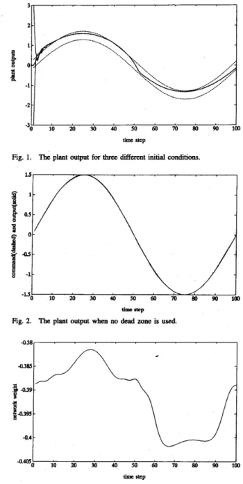
= 0.21, three initial conditions of the plant are tried: 3.0, 0.0, and -3.0. Fig. 1 shows the plant outputs for the first 100 time steps. For all of the three

initial conditions, the tracking errors are observed to converge to the dead zone after 6OOO time steps.

There are two remarks concerning the results of Part I and Part II.

Remark 1: Although a suitable dead-zone size is needed to guarantee the convergence of the tracking error to the dead zone, without using dead zone we may achieve better results in terms of how close the plant output is to the reference

CHEN AND KHALIL: ADAPTIVE CONTROL OF DISCRETE-TIME SYSTEMS

B

I

B

tl

Fig. 1. The plant output for three different initial conditions.

799 - d,=O 1.50

,

1 0.90

$

030 c 3 -0.30 -0.90

-.

m I - 8.V” 0 300 600 900 1200 1500 time step

Fig. 4. The plant output for the regulation problem when no dead zone is Used.

tim N p Fig. 2. The plant output when no dead zone is used.

command. To illustrate this point, set A = 0.30 and

4

= 0 and rerun the simulation in Part I. Fig. 2 shows that, after 6OOO time steps, only small error exists between the reference command and the plant output. The parameters, however, do not convergt. Fig. 3 shows the behavior of the typical weight w11 in f . Taking into consideration that in Part I the network weights are checked 14 digits below the decimal point for convergence, the weight fluct~atio~ in Fig. 3 should be considered very large.

Remark 2: Although Part I and Part II pertinently address o w main theoretical results in this paper, they do not illustrate the d a l role af dead-zone nonlinearity in accommodating

-1.50

I

0 140 280 420 560 700

time Step

Fig. 5. The plant output for the regulation problem when do = 0.09.

modeling errors. To emphasize this point, let us consider another example. Here neural network (60) is used to regulate the output of plant (65) to zero

We artificially construct the following situation: the bias weights in the neural network are eliminated so that

f

becomes unable to model a nonlinear function which does not vanish at the origin. The plant contains a cos term; thus, it can not be properly modeled by the neural network around the origin. The neural network is pretrained for loo0 time steps. Fig. 4 shows the simulation result when no dead zone is used. The initial condition of the plant is (yo, y-1) = (-1.5, -1.5). After some initial transient, the plant output is brought toward zero. The plant output, however, bursts into wild oscillations every time it comes close to zero. This is because the neural network controller can not provide correct cancellation control around zero plant output.

To

cope with this situation, a dead zone of size do

>

0 is specified in the updating rule. Fig. 5 shows the result when do = 0.09. After some fast initial transient, the plant output is observed to gradually decay toward the origin and finally stay at 0.09. It is interesting to turn to Fig. 6

to look at the behavior of a randomly chosen weight in the ne& network model. When

4

= 0.09 is specified, the weight converges to a constant. Fig. 6 also shows that the same weight

IEEE TRANSACTIONS ON AUTOMATIC CONTROL, VOL. 40, NO. 5, MAY 1995

- d,=O do=0.09

0 400 800 1200 1600 2000

time step

Fig. 6. The effect of dead zone on the behavior of a randomly chosen weight.

*o.w

-

- - _

-

_ _ _ OM4 a M q y ht arngu - 120 I I 0.72 c

i

OZ4

$

-024 -0.72 -120 0 160 320 480 640 eo0 time step

Fig. 7. The pendulum output.

moves around without settling to any point when

6

= 0, i.e., when no dead zone is used.

PurtZZZ: In this part we are going to apply the neural network to control a pendulum, which is a relative-degree- two system. Suppose that the equation of motion of the pendulum is

(66) Let T denote the sampling period. Equation (66) is discretized (using Euler’s Rule) as

e ( t )

+

i ( t )

+

sin ( e ( t ) ) = u(t).

& + 1 = (2 -

q e k

+

(T

-

i)ek-l

- T 2 sin (6k-1)

+

T2uk-l. ₍₆₇₎ To define the control, the same transformation as described in Sation 11 is performed

ek+2

= (2 - T)ek+l

+

(T

- 1)& - T2sin(&)

+

T ~ U ~ = ( 2 - T ) [ ( 2 - T ) &

+

(T - 1 ) e k - l - T2sin(&-1)

+

T2tik-l]

+

(T

-

1)&

-

T28an(8k)

+

T2Uk

which is modeled by

&+2 = f [ 8 k t & - i , ~ k - i , ~ ( k ) ] +jhl~uk (68)

where

3

is a neural network that contains two hidden layers with only two newms in each hidden layer, while g is a scalar

that is updated directly. At each time step, tbe cofftml U k is

-OB1

t

-0.02 I

0 320 640 960 1200 1600

trine step

Fig. 8. After some initial transient, the weight converges.

generated from (68). The updating of the weights is based on the error between &+I and

=

j[ek-l,

w - ~ ,

~ ( l c ) ]

+

B ~ - ~ u ~ - ~ (69)

as was outlined in Section ID. Figs. 7 and 8 show the simula- tion results when T = 0.3 and a dead zone of size

6

= 0.09

is used. The plant output is supposed to track a sinusoidal reference command of magnitude 1. Before the network is used for controlling the pendulum, it is trained for 12 OOO time

steps. The initial condition of the pendulum is 80 = - 1 radian. The plant output, shown in Fig. 7, converges toward the dead zone quickly after the control process starts. The behavior of a randomly chosen weight in the neural network is shown in Fig. 8. The weight converges after some initial quick changes.

V.

CONCLUSIONS

The use of neuralnetworks in control has drawn much interest in the control community in the past few years. In this work we presented an analytical study of the use of multilayer neural networks in the control of a class of nonlinear discrete- time systems with relative degree possibly higher than one. The convergence result of this paper is local with respect to the initial paramem but nodocal with respect to the initial states of the plant. This feature of the result distinguishes it from a simple local result that could have been obtained

by Taylor linearization about an equilibrium point and a set

of nominal parameters. The fact that the initial states of the plant are allowed to belong to any compact set required a carem Lyapunov-type analysis of the closed-loop system. On

the other hand, having a local result with respect to the initial parameters is not the best that one would have hoped for. In the lack of analytical results in the ma, however, the result we

obtained here is definitely a welcome conceptual contribution. The result, actually, is a little bit more than a conceptual one. The need to start from initial parameters suflicienfly close to the exact ones can be addressed by pretraining. In all our simulations, the neural network used to model an unknown nonlinearity has gone through intensive &-line t*lining using the backpropagation algorithm. This off-line training provided a good starting point when the network was used in on- line adaptive control. The idea of performing off-line training

CHEN AND KHALIL: ADAPTIVE CONTROL OF DISCRETE-TIME SYSTEMS 801

performed on a prototype sample of the system. When the network is then U& in an on-be adaptive control system, it

may not provide an acceptable model of the actual nonlinearity of the system, but it could p v i & a m-1 that is good enough for the initial parameters to be within their domain of attraction.

Our analytical study has also pointed out ithe need to incorporate a &ad-zone nonlinearity to account for modeling errors between the actual nonlinearity and its neural network model. We have demonstrated via simulations the crucial role played by the dead-zone nonlinearity.

The convergence result we obtained in Theorem 1 is stated in

a

generic farm that could be applied to many nonhear pa”e$e&ation schemes, provided the stated assumptions are satisfied. In particular, any function approximator that would

satisfy Assumption 3 with arbitrarily small E would be a

scheme to which we could apply Theorem 1. The link between our work and multilayer neural networks comes at three points. First, we used the well-known results on the use of the multilayer neural network as a universal function approximator to justify Assumption 3. Second,

ow

updating d e requires the calculation of a Jacobian matrix which can be calculated using the routines of the backpropagation algorithm. This is particu- larly important because those routines have the advantage that when the number of neuron layers is fixed (in practice, less than four layers are used), the computation time of the. Jacobian is independent of the network complexity (that is, the number of neurons used in each layer which increases with the com- plexity of the approximated function), provided appropriate parallel computing hardware is available. Third, all our simu- lations have been for the case of multilayer neural networks.

The fact that Theorem 1 is stated in a generic form that i s not limited to multilayer neural networks is a good feature and a bad feature at the same time. It is good because our analysis could be useful in other situations. But, it is bad because the analysis does not take advantage of properties that might be unique to multilayer neural networks. It is not clear at this time what could be such properties or how could they be used to obtain sharper results.

mFERJ3NCES

[l] D. G. Taylor, P. V. Kokotovic, R. Marino, and I. Kanellakopoulos, “Adaptive regulation of nonlinear systems with unmodeled dydamics,” IEEE Trans. Automat. Contr., vol. 34, no. 4, pp. 405-412, A p r . 1989.

[2] R. M. Sanner and J.-J. E. Slotine, “Gaussian networks for direct adaptive control,” IEEE Trans. Neural Networks. vol. 3, no. 6, pp. 837-863, Nov.

1992.

[3] S. S. Sastry and A. Isidori, “Adaptive control of h&zable systems:’

IEEETrans. Automut. Contr., vol. 34, no. 11, pp. 1123-1131, Nov. 1989.

[41 I. Kanellakopoulos, P. V. Kokotovic, and A. S . Morse, “Adaptive output

feedback control of a systems with output wnlinearities,” IEEE Trans. Automat. Contr., vol. 37, no. 11, pp. 1666-1682, Nov. 1992.

[51 9. Rumelbart, G. E. Hinton, and R. J. Williams, “Learning internal rep-

resentations by e m r propagation,” in Parallel Diftributed Processing, vol. 1, Rumelhart and McClelland, Ed. Cambridge, MA: MIT Press,

1986.

161 IEEE Contr. Syst. Mag., special issues on neural network control systems, 1988-1990.

[71 K. S. Narendra and K. Parthasamthy, “Identification and control of dy- namical systems using neural networks,” IEEE Trans. Neural Networks, vol. 1, pp. 4-27, Mar. 1990.

[81 F.-C. Chen, “Back-propagation neural networks for nonlinear self-tuning

adaptive control,” IEEE Contr. Syst. Mag., Special Issue on Neural Nemorks f o r C o m l Systems, Apr. 1990.

[9] R. Hecht-Nielsen, “Theory of the back-propagation neural network,” in

Proc. Int. Joint Con$ Neural Networks. June 1989, pp. 1-593-605.

[ 101 K. Funahashi, “On the approximate realization of continuous mappings by neural networks,” Neural N e w r k s , vol. 2, pp. 183-192, !989.

[11] G. Cybenko, “Approximaton by superpssitiom of a sigmo1dd func-

tion,” Dept. Elec. Computer Eng., Univ. Illinois at Urbana-Champaign,

Tech. Rep. 856, 1988.

1121 K Horn&. M. Stinchcombe, and H. White, “Multilayer feedforward networks are universal approximatorS,” Neural Networks, vol. 2, pp.

359-366, 1989.

[13] F.-C. Chen and H. K. Khalil, “Adaptive control of nonlinear systems using neural networks,” Int. J. Contr., vol. 55. pp. 1299-1317, 1992. [14] G. Kreisselmeier and B. Anderson, “Robust model reference adaptive

control,” IEEE Trans. Automat. Contr., vol. AC-31, no. 2, pp. 127-133, Feb. 1986.

[15] G. C. Goodwin and K. S. Sin, AQqptiw Filtering, Pwdiction and

CoAtnoL Englewood Cliffs, NJ: Pm~tice-Hall, 1984.

[16] K J. Astrom and B. Wittenmark, Adaprive Contml. Reading, MA: Addison-Wesle , 1989.

[17] S . Monaco andb. Nonnand-Cyrot, W%”Minim-phase nonlinear discrete- time systems and feedback s t a b i i o n , ” in P m . 1987 IEEE Con$ Deck. Contr., 1987, pp. 979-986.

[lg] S. Sastry and M. Bodson, -live Control: Stability, Convergence, and Robudrness. Englewood Cliffs, NJ: Prentice-Hall, 1989.

hr-Chupn(~ Cben (S’88-M’W) was born in I- Lan, Taiwan, Republic of china on Dec. 30,2960.

He received the B S . degree in power mechanical

engineering fmn National Tsing Hua University,

Taiwan, ROC. in 1983. After the two-year military

&?rvice in Taiwan, he tben attended .the Michigan State University and received the M.S. degree in systems science and the Ph.D. degree in electrical engineering in 1986 and 1990, respectively.

Since 1990, Dr. Chen has been on the faculty

of control engineering, National Chiao-Thg Uni- versity, Taiwan, ROC. En the past few y-, he has worked on problems related to singular perturbation thmry, airplane auto pilot design, Ho0 thmry, neural networks and adaptive control. His current research interests include the experimental phase of learning control problems involving neural networks and image feedback.

HasSan K. Khalil (S’77-M’7&SM85-F’89) re- ceived the B.S. and the M.S. degrees from Cairo

Univdty, Cairo, Egypt, and the Ph.D. degree from

the University of Illinois, Urbana-Champaign, in

1973, 1975, and 1978, respectively, all in electrical engineeting.

Since 1978, he has been with Michigan state University. East Lansing, where he is currently Pro- fessor of Electrical Enghwring. He has consulted for G e n d Motors and Delco Roducts.

Dr. Khalil has published s e v d papers on sin-

gular ptwbatiion “Is, decentralized contml, robustness, and nonlinear control. He is author of the book Nonlinear Sysrem (New York Macmillan,

1992), coauthor with P. Kokotovit and J. O’Reilly, of the book Singular Perfurlmiiovr Methods in Conhvl: Analysis and Design (New York: Academic, 1986), and coeditor, with P. Kokotovit, of the book Singular Perfurbation in Systems and Conrr~l (New York: IEEE Press, 1986). He was the recipient of the 1983 Michigan State University Teacher Scholar Award, the 1989 George S. Axelby otltstanding Paper Award of the IEEE TRANSACIIONS ON A ~ M A T I C C o m ~ a , the 1994 Michigan State University Withrow Distinguished Scholar

AwaFd, and the 1995 Michigan State University Distinguished Faculty Award. He served as Associate. Editor of IEEE TRANSACTIONS ON A m - CONTROL, 1984-1985; Registration chairman of the IEEECDC Conferewe, CDC Conference, 1986; Finance chairman of the 1987 America Control Conference (ACC); Program Chainnan of the 1988 ACC; Pmgram Committee member, 1989 ACC; and General Chair of the 1994 ACC. He is now serving as Assocrate Editor of Automatka.