joumalof
statistical
planning
Journal of Statistical Planning and and inference
E L S E V I E R Inference 64 (1997) 205-229
Bayesian analysis of growth curves with AR(1) dependence 1
Jack C. Lee*, Y.L. H s uInstitute of Statistics, National Chiao Tung University, 1001 TA Hsueh Road, Hsinchu, Taiwan 30050, ROC Received 19 January 1996; received in revised form 23 December 1996
Abstract
In this p a p e r we c o n s i d e r Bayesian analysis of the generalized g r o w t h curve m o d e l w h e n the c o v a r i a n c e m a t r i x ,~ = tr2C where C = (pli Jl), a2 > 0 a n d - 1 < p < 1 are u n k n o w n . W e c o n s i d e r b o t h p a r a m e t e r e s t i m a t i o n a n d p r e d i c t i o n of future values. Results are illustrated w i t h real a n d s i m u l a t e d data. © 1997 Elsevier Science B.V.
Keywords: Predictions; N o n i n f o r m a t i v e priors; T r a c e T d i s t r i b u t i o n
1. Introduction
We consider a generalized multivariate analysis of variance model useful especially for many types of growth curve problems. The model was first proposed by Potthoff and Roy (1964) and subsequently considered by many authors, including Rao (1965, 1966, 1967, 1977, 1984, 1987), Khatri (1966, 1973), Grizzle and Allen (1969), Geisser (1970, 1980, 1981), Lee and Geisser (1972, 1975, 1996), Fearn (1975), Lee (1982, 1988c, 1991), Jennrich and Schluchter (1986), among others.
The generalized growth curve model is defined as
Y = X z A + ~ (1.1)
pxN p x m m x r r × N pxN
where z is unknown and X and A are known design matrices of ranks m < p and r < N, respectively. The columns of ~ are independent p-variate normal, with mean vector 0
Research Supported in Part by NSC grant 84-2121-M009-008. The authors thank A. Chao, a referee and an associate editor for some helpful comments on an earlier version of the paper, K.C. Liu and W.F. Niu for programming support.
* Corresponding author, e-mail: [email protected]
0378-3758/97/$17.00 © 1997 Elsevier Science B.V. All rights reserved PII S 0 3 7 8 - 3 7 5 8 ( 9 6 ) 0 0 1 4 4 - 9
206 J.C Lee, Y.L. Hsu/Journal of Statistical Planning and Inference 64 (1997) 205-229
and c o m m o n covariance matrix X. In general, p is the number of time (or spatial) points observed on each of the N cases, m and r, which usually specify the degree of polynomial in time (or space) and the number of distinct groups, respectively, are assumed known• The design matrices X and A will therefore characterize the degree of the growth function and the distinct grouping out of the N independent vector observations• Potthoff and Roy (1964) gave many examples of growth curve applica- tions for the model (1.1). Grizzle and Allen (1969), Lee and Geisser (1975), Rao (1977, 1987) and Lee (1988c), Chi and Reinsel (1989), among others, applied the model to some biological data. Lee (1988a) and Keramidas and Lee (1990) applied the model to the forecast of technology substitutions•
In Lee (1988c, 1991) and Keramidas and Lee (1990, 1995) the importance of the AR(1) dependence, or serial covariance structure, was demonstrated repeatedly for the covariance matrix X for the model (1.1). When the AR(1) dependence holds for X, we have 2; = o - 2 C , where C = (pli-sl), for i , j = 1, ..., p, 0 .2 > 0 and -- 1 < p < 1 are
unknown. The estimation of the parameters and prediction of future values for this model have been so far based on the method of maximum likelihood (ML), which is optimum in large sample. The purpose of the paper is to consider this model from a Bayesian point of view hoping that a more practical solution can be furnished when the sample size is relatively small. Indeed, several published data sets are relatively small in their sizes. We will compare our results with those based on the M L method via real and simulated data sets.
The serial covariance structure is defined as
X = o ' 2 C , (1.2)
where C = (pli sl), i , j = 1 . . . p, i.e.,
C = ~ ! .... p - 2 (1.3)
p i l p ; - 2 ...
and a 2 > 0 and - 1 < p < 1 are unknown. It is conceivably one of the most impor- tant covariance structures for the generalized growth curve model.
In addition to the inferences on the parameters z, a 2 and p, we will also consider several types of prediction problem for the growth curve model as specified by (1.1)-(1.3). Let V be a set of p x K future observations drawn from the generalized growth curve model, i.e. the set of future observations are such that given the parameters z and I;,
E ( V ) = X z F , (1.4)
where E() denotes expected value, F is a known r x K matrix, and the columns of V are independent and multivariate normal with a c o m m o n covariance matrix X.
J.C. Lee, EL. Hsu/dournal of Statistical Planning and Inference 64 (1997) 205-229 207 Geisser (1970, 1980) and Lee (1982) considered prediction of V, given Y as the sample, from a Bayesian viewpoint. Lee and Geisser (1972, 1975), Fearn (1975), Rao (1975), and Lee (1988c, 1991) considered the problem of predicting ~2), given i1(1) and Y, if Vis partitioned as V = (V (1)', V(2)') ,, where V (i) is pi x K (i = 1, 2) and p~ + P2 = P. If p is interpreted as the number of points in time being observed, then the problem is mainly concerned with predicting the generalized growth curve for future cases for the same set of p time points, or a subset of size P2. When P2 < p and K = 1, it is also called the
conditional prediction
of the unobserved portion of a partially observed vector.The third prediction problem is somewhat different. It is concerned with predicting the future values of the observed cases. Let y, of dimension q x n, be a set of n ( ~< N) future q-dimensional observations whose previous p-dimensional observations are a subset of E We are interested in predictingy given E This is a time series prediction and thus is important in practice. This type of prediction is called the
extended
prediction
of y, because the prediction is made beyond the observed time range of the sample E The extended prediction o f y was considered by Lee (1988c) and Keramidas and Lee (1990, 1995).In Section 2, Bayesian estimation of the parameters is considered. Section 3 is concerned with three types of prediction problem. The results developed in the paper are illustrated in Section 4 with real and simulated data. Finally, some concluding remarks are given in Section 5.
2. Bayesian estimation of parameters
F o r the sake of convenience we shall deal with the pseudo-augmented model
e ( r ) : \ w (2.1)
The likelihood function of ~, a 2 and p given Y is
L(z, rr 2, PlY) oc a-Pn(1 --
p2)-(p-1)N/2x e x p { - - 2 ~ t r C - I [ Y - ( X , Z ) ( o ) A I [ Y - ( X , Z ) ( ; ) A I '
}.
(2.2) F o r the prior of ,, a 2 and p, we will use the following noninformative prior
1
g('L', 0 "2, p) OC ~-'~. (2.3)
In (2.3), we have assumed that ~, a 2 and p have independent prior distributions and no information is available for each of the parameters. This is in the same spirit as Zellner and Tiao (1964).
208 J.C Lee, Y.L. Hsu/Journal of Statistical Planning and Inference 64 (1997) 205-229 Hence, the posterior density of ~, tr 2 and p given Y is
P(~, a 2, plY) oc
a-tvN+ 2)(1 --p2)-(v-1)N/2
x e x p { - - 2 ~ t r C - I [ Y - - ( X , Z ) ( o ) A I [ Y - ( X , Z ) ( o ) A I } .
(2.4) Integrating out a 2 and using Lemma A.1 and the application of some algebraic identities yield P(x,
PlY) oc
(1 - p2)-(p-,)N/2 SIPN/2,
(2.5) where $1 = tr(X'C- 1X)(~ - ÷)AA'(~ -- ÷)' + b,÷ = (X'C- ' X ) - 'X'C- 1YA'(AA')- 1,
(2.6) b = tr(X'C1X)- 1X'C- 1SC- 1X + tr(Z'CZ)- 1Z'YY'Z,
s = YES - A ' ( A A ' ) - 1A] r ' .By Theorem A. 1, it is clear that conditional on p,
[p ,-, Tr(÷,
AA', b, X'C- 1X, pN).
(2.7)m × r
Moreover, integrating out • from (2.5) we have
P(p[Y) oc b-~pN- mr)/2 IX'C-
1X[ r/2(1 -- p2)-~p-1)N/2.
(2.8)Since
P(~, p l Y ) = P(~[p, Y)P(pIY)
and P(xIY)=~P(~, plY)dp,
the integral can be approximated byP(TI
Y) -- P(~ld, Y),
(2.9)where ¢3 is the mode of
P(plY),
ifP(plY)
is concentrated and nearly symmetric, as pointed out by Ljung and Box (1980). Of course, the integration can be performed numerically as the one-dimensional integral can be done rather accurately.Hence, we have the following posterior distribution of ~:
P(~IY)- Tr(÷*,
AA', b, X'C- 1X, pN),
(2.10)where
~* = (X'C- I x ) - l x t c , - I y A t ( A A t ) - 1,
b = tr(X'~'- 1X)- 1X'C- I S C - 1X + tr(Z'CZ)
1Z'YY'Z,
(2.11)= ( ~ , ' - J , ) ,
/3 maximizes
P(plY),
as given in (2.8).J.C. Lee, Y.L. Hsu/Journal of Statistical Planning and Inference 64 (1997) 205 229 209
Integrating w.r.t, z in (2.4) and using arguments similar to (2.9), we obtain the following approximation for the posterior distribution of tr 2,
P ( a 2 I y ) - I G ( P N - m r ~ ) 2 , , (2.12)
where b is given in (2.11) and IG(va, v2) is the inverse gamma distribution with parameters vl and v2.
By Theorem A.3 and the fact that if V ~ Beta(½v2, ½vl) and F ~ F ( v l , v2), then V = v2/(v2 + v~F), 1 - ~ posterior region for z can be obtained from the following inequality:
- l t r ( X ' ~ ' - ~ X ) ( z - ÷*)A,4'(z - ÷*)' <<. m r F1 ~(mr, p N - mr) (2.13) p N - mr
where F~_~(v~, v2) is the upper 100e percent point of the F-distribution.
F o r the special case in which r = 1, we have the following 1 - ~ posterior region for z:
m
N b - ~(z - ~ * ) ' ( X ' C - I X ) ( z - ~*) <~ F~ _~(m, p U - m), (2.14) p N - m
and ÷* are given in (2.11).
3. Prediction
Three types of prediction for the model specified by (1.1)-(1.3) will be considered in this section.
3.1. P r e d i c t i o n o f the w h o l e f u t u r e m a t r i x V
The prediction of the future matrix V, p × K, given the sample, Y, p × N, is considered here. Schematically, the matrices Y and V are shown below.
N K
The density function of V given z, o 2 and p is
[1
]
f ( V I z , ~r e, p ) oc a vx(1 - p2)-(v- l~K/Zex p -- }--~2 tr C - I(V -- X r F ) ( V - X z F ) ' .
2 1 0 J.C. Lee, EL. Hsu/Journal of Statistical Planning and Inference 64 (1997) 205-229
U p o n combining with the posterior density of ~, a z and p as given in (2.4), and integrating out a2, we have
P(V, "c, p l Y ) oc (1 - p 2 ) ( p - 1 ) ( N + K)/Z s 2 P ( N + K)/2 ' (3.2)
where
$2 = t r C - ~ ( Y - - X ~ A ) ( Y - - X x A ) ' + t r C I ( V - - X x F ) ( V - X x F ) ' , = tr C l(Yo - XZAo)(Yo - X~Ao)',
Yo = (Y V), (3.3)
Ao = (A V).
By L e m m a A.1, we obtain
$2 = bo + trAoA~(~ -- ÷o)'(X'C- 1X)(~ - ~o), (3.4) where
bo = tr(X' C - aX) ~X' C - lSoC- 1X -~- t r ( Z ' C Z ) - tZ'Yo Y~Z,
So = Yo[I -- Ao(AoA'o)- ~Ao] Yo', (3.5)
÷o = ( X ' C - 1X)- I X ' C - I roA'o(AoA'o)- 1. Integrating out ~, we have
P(V, PlY) oc bo(P(N+K)-mr)/2~¥'C XXl-r/2(1 - p Z ) - ( p 1)(N+K)/2. (3.6) By (4.12) of Geisser (1970),
So = S + ( V - Y A ' ( A A ' ) - a F ) M ( V - Y A ' ( A A ' ) - I F ) ' , (3.7) where M = I - F'(AoAo)-XF, and it can be shown that
bo = b + tr M ( V -- X ÷ F ) ' C - 1X(X'C- ~X)- ~X'C- a(V - X ~ F )
+ tr(V - X ~ F ) ' Z ( Z ' C Z ) - ~Z'(V - X ÷ F ), (3.8) where ~ is given in (2.6).
We will consider the special situation in which r = 1. In this situation F = 1 and M is a constant. Integration w.r.t. V yields
P v ( p l r ) ~ b -tpN m,~/2161-K/2 IX'C-1xI-r/2(1 - - p2)-tp-1)tN+K)/2 (3.9) where
,LC Lee, EL. Hsu/Journal of Statistical Planning and Inference 64 (1997) 205-229 211
With arguments similar to (2.9), we obtain the following approximation for the predictive distribution of V: P ( V I Y ) - Tr(X÷vF, 1, by, C,v, p(N + K) - mr), (3.11) where ~V ~- ( X ' ~-*v l x ) - 1 X ' e v 1 Y A ' ( A A ' ) - 1, bv = tr(X'Cv 1X)- 1X'Cv 1S~'v 1X + tr(Z' CvZ)- IZ' Y Y ' Z ,
Gv = M~; lX(X' ~ 'X)- ix' ~ ' + Z(Z'~vZ) ~Z',
(3.12)
j3v maximizes Pv(PFY) as given in (3.9).
It is noted that Zv and ~ are different because (3.9) is different from (2.8). Thus, the future matrix V has a trace T distribution.
3.2. Conditional prediction o f V t2) given V ¢1) and Y
We next consider the conditional prediction of V tz) given V tl) and Y, if V is partitioned as V = (V ¢a)', V¢2)') '. Schematically, we have the following:
V(~)
Y
V(2)
where Y, p x N, is the complete sample; V (~), pa × K, is the partially observed matrix and V (2), P2 × K, is the unobserved portion to be predicted. Of course, Pl + P: = P. From Eq. (3.6), it can be shown that
P ( V (2), p [ V (1), Y ) cxl (1 - p Z ) - ( p i)(N+K)/21XtC-1X[-r/2 x [bl + (V (2) - IT"(2))'G22(V (2)- I7'(2))] (p(N+K)-m~)/2,
(3.13)
where G = M C - 1 X ( X ' C - 1 X ) - 1 X ' C - 1 ~_ Z ( Z t C Z ) - 1Zt ' bl = b + ( V (1) - X(1)÷F)'G11.2(V (1) -- X(1)'~F), ~,~-(2) -- X(2),~F __ -- G~-I G 2 1 ( V ---(1) - - X ( 1 ) ~ F ) , X = (X (l)', x(E)') ' , (3.14) ( G l l G21"~ G = \ G 1 2 G22 j , Gij is Pi × P j , G l l . 2 ~ G i l --G12G2~G21.
212 J.C. Lee, Y.L. Hsu/Journal of Statistical Planning and Inference 64 (1997) 205-229 Integrating over V (2), we have
P(pIV (1), Y ) oc (1 - p 2 ) - ( p - 1)(N + r)/21X,C-1XI ,/2 b~(pN + plK-mr)/ZlG221- P212" (3.15)
With arguments similar to (2.9), we obtain the following approximation for the conditional distribution of V TM given V (1) and Y:
p(V(2)IV(1), y ) - T r ( l ? ( 2 ) * , 1, bl, (722, p(N + K ) - mr), (3.16) where I~(2) * = x ( z ) , ~ I F __ (~221 G Z l ( V (1) - X ( 1 ) , ~ I F ) , t)1 = ~ + (VO) - X ( 1 ) ' ~ I F ) ' G 1 1 . 2 ( V O ) - X ( I ) ' r l F ) , ~1 = (X'C*-IX) - 1X' C* I Y A ' ( A A ' ) - i , C, = M C * IX(X' C* I X ) - 1X'C*-' + Z ( Z ' C * Z ) - 1Z', (3.17)
Gij is defined as Gij,
and/31 maximizes P ( p l V (1), Y ) as given in (3.15).
Thus, the predictive inference on V (2) given V (1) and Y can be based on the trace
T distribution. Alternatively, P(V(2)IV(1), Y ) can be obtained from (3.13) by integrat- ing over p numerically, i.e., P(v(E) I V m, Y ) = 5P(V (2), p l V (1), Y ) d p .
3.3. Extended prediction of y
We now consider the extended prediction of y, given Y. This is a time-series prediction which is of practical interest for many types of growth curve data. In order to make this type of prediction the covariance structure generally has to be extendable to the future values of the individuals observed.
Let x, q x m , be a design matrix corresponding to y, Y = ( Y I , ..., YN),
A = (/11 .. . . ,AN),y = (Yl . . . . ,y,), and assume that for i ~< n,
and
J.C Lee, Y.L. Hsu /Journal of Statistical Planning and Inference 64 (1997) 205 229 213
where
(c1, c,2"
C2~ C 2 2 / = ( P l " - b l ) '
a, b = 1 . . . ( p --[- q), C,1 is p × p, C12 is p x q, C22 is q x q, and C21 = C12. Schemati- cally, Y a n d y are s h o w n below:
N
q Y I
n
F o r the extended prediction of y, given Y, we will consider the special situation in which r = n = 1. This is g o o d enough, in practice, because conditional on the k n o w - ledge o f ~ a n d X, y l . . . . , y , are independent. W e will consider the situation in which Yi will be excluded f r o m the s a m p l e w h e n Yi is being predicted. Thus, in this s t u d y the s a m p l e is Y(i) which is Y ( i ) = ( Y 1 . . . Y i - l , Yi+l, . . . , Y u) a n d let Yi* : ( Y i ' , Y ' ) ' , X * = ( X ' , x ' ) ' and A , ) = (A1, . . . , A i 1,AI+1, -.-,AN).
C o m b i n i n g the density of Yi* with the p o s t e r i o r of z, a 2 and p given Y,) a n d integrating o u t a 2, we h a v e P(YI*, z, PlY(i)) ~: (1 - p2) ((p- 1)N+q)/2S3(PN+q)/2 ' (3.20) where S 3 --- 9 2 + ('r - - + ) ' Q ( z - +), b2 = (+1 - +2)'QIQ-1Q2(+l - +2) + t r ( Z * ' C Z * ) - ~ z * ' Y i * Y i * ' z * + t r ( Z ' C l l Z ) -1 z Y(i) Y(i)z + t r ( X ' c[~ ~ X ) - 1 x ' c [ t ~ s(1)c[11X, , , Q1 = ( N - 1 ) X ' C l l l X , Q2 = X * ' C - 1 X * , Q = Q1 + Q2, (3.21)
S<O -- Y<i)[I -- A~i)(A~oAII))-1A(i)] V<i), +1 = ( X t C l l 1 x ) - 1X t C l l 1 Yti)A(i)(A(1)Aii)) - i , +2 = ( x *' c - ' x * ) - l x * ' c - 1 Yi*A', ( A i A I ) - 1,
+ = Q - a ( Q I + 1 +
Q2+2),
214 J.C Lee, EL. Hsu/Journal of Statistical Planning and Inference 64 (1997) 205-229 Integrating over z yields
P(p, Yi*lr(i)) oc (1 -- p2)-(~p- 1)N+o)/2[Q[ 1/2b2ft, fN 1)+q-mr)/2, (3.22) where G* = C- i x * (X*'C- 1X*)- ' Q , Q - 1 O 2 ( X * ' C - 1 X * ) - ' X * ' C - 1 jr_ Z * ( Z * ' C Z *)- ' Z *',
6;, = (6;t,
6;t2
\6;7, 6;t2)'
6;*,.2 = 6;*, -- v12"~22 u 2 1 , e , ~ , - ' ,,z_, (3.23)b2 = b.) + (Yi -- X÷IAi)'G*,.2(YI - X ÷ l A i ) + (Yi - fii)'G*2(Yi --.Vi),
: t ] t t
bti ) t r ( X ' C ; I ' X ) - a X ' C ? a l s , ) c x , I X + tr(Z C l l Z ) Z Y.)Y.)Z,
fii = X'~lAi -- G22 G21(Yi-- X ~ l h i ) .
By arguments similar to (2.9), we have the following approximate predictive density of Yi given Y,
P(y, I Y ) - Tr~i*, 1, ~o + (Y~ - X ' ~ * ) ' 4 t , . z ( Y , - X ÷ * ) , 4*2, p ( N - 1) + q - mr),
(3.24) where ; * = x ' r * A i - - 6;22^* 1 ^ , 6 ; 2 1 ( Y i - - X + t A i ) , +1" = ( X t C l , 1 X ) ' X t C l l ' Y,)AIi)(A<i)A~o)-', G* = C - ' X * ( X * ' ~ ' - I x * ) - I O I O - I O 2 ( X * ' C - I X * ) ' X * ' C - ' + Z * ( Z * ' C : Z * ) xz*', ~.) = t r ( X ' C ; , ' X ) ' X ' C ; a ' S , ) C ? , ' X + tr(Z'~'l , Z ) - ' Z'Y.)Y(i)Z; (3.25) ~3r maximizes
Py(PIY) oc (1 - p2) u,- ,)~N- ,)/2[Cl- U2lG,2l-1/21Ql-1/2[b,) + (y~ _ X~lAi),
X G*I.2(Y i -- X.rlAi) ] -(p(N- 1)-mr)/2 (3.26)
4. Numerical results
This section is devoted to the illustration of the conditional prediction of V (2) given V tl) and K and the extended prediction o f y given Y. For the conditional prediction, we will follow Lee and Geisser (1975), Fearn (1975) and Lee (1988c) in setting K = 1,
J.C. Lee, Y.L. Hsu/Journal of Statistical Planning and Inference 64 (1997) 205 229 215
P2 = 1 and Pl = P - 1, that is, we will predict the last observation of the partially observed vector. F o r the extended prediction, we will set q = 1 and n = 1, that is, we will predict one future c o m p o n e n t at a time.
4.1. Simulations
In this subsection we will present some simulation results regarding the p a r a m e t e r estimation for ~ and p, the conditional prediction of V (2) given V (1) and Y, and the extended prediction o f y given Y for the special situation in which r = 1 and K = 1. The posterior region for ~ can be obtained from Eq. (2.14). Meanwhile, from Lee (1988c, 199l), we can also obtain an a p p r o x i m a t e confidence region for T. F r o m the asymptotic result of +, the M L E of ~, we have
COV(+)~" o ' 2 ( X ' C - l X ) -1 ( ~ ( A A ' ) 1, t r ( X @ 1X)(~ - ÷)AA'(~ -- ÷)' &2 -,~ Z2r as N ~ Go. (4.1) Hence, p r [ t r ( X @ - 1X)(~ - ÷)AA'(~ - ~)' ] L 62 ~ zE~(ct) = 1 - ~. (4.2)
Since AA' = N, we have the following 1 - ~ confidence region:
(~ - ÷ ) ' ( X @ 1 X ) ( ~ - ~) <~ c2,
(4.3)
where if2 2 0¢ c~ = ~ z m , ( ) , '~ = (X'C- IX)- 1XtC-1 Y A t ( A A ' ) - 1. ~2 = [ t r ( X @ - l x ) 1X, ~ 1S~ 1X + t r ( Z @ Z ) - I Z , y y , z ] / p N , (4.4)and fi maximizes the profile likelihood function
Lmax(P) = (¢~2(p)) pN/2(1 __ p2)-~'(p 1)/2
(4.5)
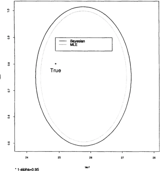
In order to c o m p a r e the regions for • obtained by the two different methods, the values for N, p, ~, ~, ~r 2 and p are given in Tables 1 and 2. F r o m the tables, it is clear that the percentage of the M L regions covering the true values is consistently smaller than 0.95. The corresponding Bayesian regions are much better, because the percent- age is closer to 0.95 for each of the 12 situations. This explains the p h e n o m e n o n in
216 J.C. Lee, EL. Hsu/Journal of Statistical Planning and Inference 64 (1997) 205 229 Table 1
Comparison of coverage probabilities between ap- proximate confidence region and Bayesian region for z ( m = 2 , r = l ) N p Coverage probability Bayesian ML 5 0.5 0.944 0.883 5 0.8 0.934 0.872 10 0.5 0.958 0.942 10 0.8 0.918 0.886 15 0.5 0.955 0.938 15 0.8 0.942 0.923 Note: p = 4, 1 -- c~ = 0.95, z = (25, 0.8)', cr z = 5 and no. of replications = 1000. Table 2
Comparison of coverage probabilities between approximate confidence region and Bayesian region for z (m = 3, r = 2) p Coverage probability Bayesian M L N1 = N2 = 5 0.5 0.936 0.842 NI = N2 = 5 0.8 0.919 0.823 Na = N2 = 10 0.5 0.940 0.905 N1 = N2 = 10 0.8 0.934 0.891 N1 = N2 = 15 0.5 0.954 0.932 N1 = Nz = 15 0.8 0.952 0.932 p = 4, 1 - ~ = 0.95, • = (22 3 0.27 0.26"]' Note: 2012 1.03 --0.01 ] ' \
cr 2 = 5 and no. of replications = 1000.
F i g . 1 i n w h i c h t h e c o n f i d e n c e r e g i o n f o r z is s m a l l e r t h a n t h e p o s t e r i o r r e g i o n . T h i s a l s o i n d i c a t e s t h a t t h e a s y m p t o t i c t e s t b a s e d o n t h e l i k e l i h o o d r a t i o c r i t e r i o n will b e b i a s e d t o w a r d r e j e c t i n g t h e n u l l h y p o t h e s i s . T h i s t y p e o f b i a s e d n e s s h a s b e e n o b s e r v e d i n o t h e r o c c a s i o n s a s well, s e e e.g. L a i t i n e n ( 1 9 7 8 ) a n d L e e ( 1 9 8 8 b ) . W e n e x t c o m p a r e t h e c o n d i t i o n a l p r e d i c t i o n o f V t2) g i v e n V (1) a n d Y a n d t h e e x t e n d e d p r e d i c t i o n o f y g i v e n E H e r e w e s e t p = 4, c~ = 0.05, z = (25, 0.8)', p = 0.8, a 2 = 5, N = 5, 10, 15 a n d t h e n u m b e r o f r e p l i c a t i o n s g = 50. F o r t h e c o n d i t i o n a l p r e d i c t i o n , w e will set K = 1, P l -- 3 a n d P2 = 1. F o r p r e d i c t i v e p u r p o s e s , w e w i t h h o l d o n e v e c t o r a n d u s e t h e r e s t a s t h e s a m p l e f o r p r e d i c t i n g t h e l a s t c o m p o n e n t o f t h a t v e c t o r a n d r e p e a t t h i s f o r e a c h o f t h e N o b s e r v a t i o n s . T h i s g i v e s N p r e d i c t e d v a l u e s f o r
J. C. Lee, EL. Hsu /Journal of Statistical Planning and Inference 64 (1997) 205-229 217 o , z ao ¢e e~
True
r - t5 t5 Lt) d i i i i i 2 4 2 5 2 6 2 7 2 8 * 1 - a l p h a = 0 . 9 5Fig. 1. Confidence and posterior regions for tau.
the last N observed values in each data set. Overall, there are 9 x N predicted values to be compared with 9 × N actual observations. The mean squared deviation (MSD), the m e a n absolute deviation ( M A D ) and the mean relative absolute deviation ( M A R D ) of the predicted values from the actual observations are used to assess the relative merits of the two methods. A comparison of prediction accuracy for V (2) given V (1) and
Y between Bayesian and M L methods is given in Table 3. It is noted that in the prediction process, V (1) is not used in deriving the parameter estimation although it is used as part of the conditional m e a n vector.
As for the extended prediction, we set the last row of the generated Y as y and the first three rows as the corresponding sample. Thus, we set p = 3 and q -- 1. Similar to
218 J.C. Lee, Y.L. Hsu/Journal of Statistical Planning and Inference 64 (1997) 205 229 Table 3
Comparison of prediction accuracy for V(2~ between Bayesian and M L methods Bayesian ML N = 5 N = 1 0 N = 1 5 N = 5 N = 1 0 N = 1 5 MSD 2.1504 1 . 9 9 8 1 1.8389 2.3752 2.0089 1.8768 MAD 1 . 1 5 0 5 1.1329 1 . 0 9 4 8 1.2304 1 . 1 4 2 3 1.1058 MARD 0.0428 0.0418 0.0402 0.0455 0.0422 0.0407
Note: p = 4, 1 -- c~ = 0.95, ~ = (25,0.8)', p = 0.8, cr 2 = 5 and no. of replications = 50.
Table 4
Comparison of prediction accuracy and coverage probability for y be- tween Bayesian and ML methods
Bayesian ML N = 5 N = 10 N = 15 N - 5 N = 10 N = 15 MSD 2.3008 1 . 9 3 7 1 1.9048 2.3585 1.9350 1.9066 MAD 1.2106 1 . 1 1 8 1 1.1009 1 . 2 3 4 1 1.1163 1.1019 MARD 0.0444 0.0412 0.0437 0.0454 0.0415 0.0404 Coverage 0.940 0.949 0.954 0.818 0.902 0.928
Note: p = 3, q = 1, 1 - c~ = 0.95, z = (25, 0.8)', p = 0.8, a 2 = 5 and no. of replications - 50. t h e c o n d i t i o n a l p r e d i c t i o n , t h e r e will b e g x N p r e d i c t e d v a l u e s t o b e c o m p a r e d w i t h 9 x N a c t u a l s . A c o m p a r i s o n o f p r e d i c t i o n a c c u r a c y f o r y g i v e n g b e t w e e n B a y e s i a n a n d M L m e t h o d s i n t e r m s o f M S D , M A D a n d M A R D is g i v e n i n T a b l e 4. I n a d d i t i o n t o t h e p o i n t p r e d i c t i o n w e will a l s o c o m p a r e t h e i n t e r v a l p r e d i c t i o n f o r y g i v e n E I n o r d e r t o c o m p a r e t h e i n t e r v a l p r e d i c t i o n f o r y , w e n o t e t h a t t h e B a y e s i a n m e t h o d is b a s e d o n a p r o p e r t y o f t h e trace T d i s t r i b u t i o n a s g i v e n i n (2.14). F o r t h e M L m e t h o d , w e will u s e t h e f o l l o w i n g a p p r o x i m a t e i n t e r v a l : "JC Zct/21~ f , (4.6) w h e r e z~/2 is t h e 1 0 0 . e / 2 p e r c e n t p o i n t o f t h e s t a n d a r d n o r m a l d i s t r i b u t i o n , ~r} = ~rZEC22 - CzlC?11C12 + H ( N X ' C ? l l X ) - I H ' + 2 C 2 ~ C [ ~ X ( N X ' C ; ~ X ) I H ' ] , (4.7) H = C 2 1 C l 1 1 X - - x .
(4.8)
J.C. Lee, EL. Hsu/Journal of Statistical Planning and Inference 64 (1997) 205-229 219
It is noted that tr] is the variance of the forecast error f o r y when the parameters are assumed known. F o r the variance of forecast error for V <2) we will use Sm~ as indicated in (3.11) of Lee (1988c):
Srn ~ =
C22
-~- (blB 2 + C 2 x ) C ( l l ( b l B z + C 2 ] ) ' - - ( b i b 2 + C 2 1 ) C l 1 1 C 1 2 ,-- C2~Ca~(bIB2 + C2~)', (4.9)
bx = F ' ( F F ' ) - F , (4.10)
n 2 = ( x - c2 ~ c ; / x ) ( x ' c ~ x ) - ~x'.
(4. ] 1)
F r o m the simulation study, we see that both methods produce similar prediction accuracy for V t2) a n d y in terms of MSD, M A D or MARD, as shown in Tables 3 and 4, respectively. The Bayesian method yields longer predictive intervals fory, as shown in Fig. 2 for N = 10, which is typical in each of the 50 replications for each N which was conducted in the simulation. Similar results are also true with the real data examined in Section 4.2, as shown in Fig. 4. However, the percentage of the Bayesian predictive intervals covering the values to be predicted are closer to 1 - ~ than the M L intervals, as seen in Table 4. This is consistent with the comparison of the regions for r. It is therefore clear that the Bayesian predictive intervals are superior to the M L intervals when the samples size N is relatively small.× X X 0 X 0 X • X 0 • 0 X X ,, X 0 X 0 0 0 0 • m, X 0 0 • • 0 X • X 0 X 0 0 0 X 0 X X X X 2 4 6 8 10 Observation
220 J.C. Lee, EL. Hsu/Journal of Statistical Planning and Inference 64 (1997) 205-229 4.2. Illustrative examples
S o m e of the results d e v e l o p e d in S e c t i o n s 2 a n d 3 a r e a p p l i e d to the d e n t a l m e a s u r e m e n t s of 11 girls a n d 16 b o y s a n d t h r e e o t h e r d a t a sets (ramus, m i c e a n d glucose data). T h e d e n t a l d a t a set, w h i c h is r e p r o d u c e d in T a b l e 5, was first c o n s i d e r e d b y P o t t h o f f a n d R o y (1964) a n d l a t e r a n a l y z e d b y Lee a n d G e i s s e r (1975), F e a r n (1975), R a o (1987), a n d Lee (1988c, 1991), a m o n g others. D e n t a l m e a s u r e m e n t s were m a d e o n 11 girls a n d 16 b o y s at ages 8, 10, 12, a n d 14 years. E a c h m e a s u r e m e n t is the d i s t a n c e , in m i l l i m e t e r s , f r o m the c e n t e r of the p i t u i t a r y to the p t e r y g o m a x i l l a r y fissure. F r o m T a b l e 5 it is clear t h a t the d i s t a n c e b e i n g m e a s u r e d can d e c r e a s e w i t h age, d u e to the fact t h a t the d i s t a n c e r e p r e s e n t s the relative p o s i t i o n of t w o p o i n t s . T h e r a m u s d a t a were o r i g i n a l l y given in E l s t o n a n d G r i z z l e (1962) a n d s u b s e q u e n t l y a n a l y z e d b y Lee a n d G e i s s e r (1975), F e a r n (1975), R a o (1987), Lee (1988c, 1991), a m o n g others. T h e m i c e d a t a were first r e p o r t e d b y W i l l i a m s a n d I z e n m a n (1981) a n d l a t e r a n a l y z e d b y R a o (1987), Lee (1988c, 1991), a m o n g others. T h e g l u c o s e d a t a were first r e p o r t e d b y Z e r b e (1979) a n d l a t e r a n a l y z e d b y C h i a n d Reinsel (1989) a n d K e r a m i d a s a n d Lee (1995). W e will p r i m a r i l y focus o n the d e n t a l d a t a , a l t h o u g h the p r e d i c t i o n results will be s u m m a r i z e d for the o t h e r three d a t a sets as well.
W e will n e x t d e a l w i t h the d e n t a l d a t a in m o r e details. Since the m e a s u r e m e n t s a r e o b t a i n e d at e q u a l t i m e intervals, the d e s i g n m a t r i x X is
X = - 3 - 1 1 '
Table 5
Dental measurements of 11 girls and 16 boys
IndividuaP Age IndividuaP Age
8 10 12 14 8 10 12 14 1 21 20 21.5 23 15 25.5 27.5 26.5 27 2 21 21.5 24 25.5 16 20 23.5 22.5 26 3 20.5 24 24.5 26 17 24.5 25.5 27 28.5 4 23.5 24.5 25 26.5 18 22 22 24.5 26.5 5 21.5 23 22.5 23.5 19 24 21.5 24.5 25.5 6 20 21 21 22.5 20 23 20.5 31 26 7 21.5 22.5 23 25 21 27.5 28 31 31.5 8 23 23 23.5 24 22 23 23 23.5 25 9 20 21 22 21.5 23 21.5 23.5 24 28 10 16.5 19 19 19.5 24 17 24.5 26 29.5 11 24.5 25 28 28 25 22.5 25.5 25.5 26 12 26 25 29 31 26 23 24.5 26 30 13 21.5 22.5 23 26.5 27 22 21.5 23.5 25 14 23 22.5 24 27.5
,I.C. Lee, Y.L. Hsu/Journal of Statistical Planning and Inference 64 (1997) 205-229 221
Also, from the findings in Lee and Geisser (1975) and Lee (1988c), the individual # 20, who is a boy, could be excluded because it is suspected to be an aberrant observation. Furthermore, from Lee (1988c, 1991) it is clear that the data should be treated as from two different populations with distinct mean functions and serial covariance ma- trices. However, for illustrative purposes, we will also include the situation in which a common serial covariance structure is assumed for measurements of both girls and boys.
Before dwelling on the prediction results we note that from Fig. 3, the posterior densities of p for different subsets of the data are all well concentrated and nearly
Den~d data Boys ~ m ( ~ n t ~ )
oi
: ~ : / i
o **
0.0 0.2 0.4 0.6 0.II o 1.0 0.0 0.2 0.4 0.II O.a 1.0
¢aO a ~
Girls date (Dental) Boys clma excluding 20~ inclividual
" - / i
"
i
i
f ,
0.0 0.2 0,4 0.6 0.8 1.0 0.0 0.2 0.4 0.6 0.4 1.0
222 ~ C. Lee, Y.L. Hsu/Journal o f Statistical Planning and Inference 64 (1997) 205 229 I • ~ MB~';InReel Orate [ x 8 o × × × o • 0 o x x • x o X • • O O X t~ O • >, O O • × O X O • O X • O X O o x o x ~ x X X • 0 X i ! i 2 4 6 8 10 Observation
Fig. 4. C o m p a r i s o n of p r e d i c t i v e i n t e r v a l s for y ( D e n t a l girl data).
symmetric. This means that the corresponding approximations for the posterior distributions of • should be quite adequate.
We begin by assuming that the girls and boys are from two different populations. The design matrixA is then a 1 x 11 vector for the girls and a 1 x 15 vector for the boys, both consisting of all l's. In case when the individual # 20 is not excluded, the design matrix A is a 1 x 16 vector of l's for the boys. When a common covariance structure is assumed for both populations, the design matrix A consists of 11 columns of (1, 0) followed by 15 columns of (0, 1) when the individual # 2 0 is excluded. In the situation in which the individual # 20 is included, then there are 16 columns of (0, 1) instead.
It is noted that when two distinct covariance structures are assumed for boys and girls, the predictions are performed separately and then the results are combined. Although the sample sizes will be smaller when compared with the c o m m o n covariance structure case, the prediction performance can be better if the two conva- riance matrices are quite different.
The comparison of predictive performance for conditional predictions of V (2) given V (1) and Y is summarized in Table6. The criteria used in the table are MSD, M A D and MARD. There are four different situations for this data set. Dental 1 is the dental data with girls and boys having identical covariance structure;
J.C Lee, EL. Hsu/Journal of Statistical Planning and Inference 64 (1997) 205-229 223 Table 6
Comparison of conditional predictions for four data sets
Bayesian ML MSD 3.0135 3.3575 Dental 1 MARD 0.0499 0.0527 MAD 1.0296 1.0741 MSD 1.8594 1.9583 Dental 2 MARD 0.0395 0.0414 MAD 1.2899 1.3596 MSD 2.1636 2.5070 Dental 3 MARD 0.0432 0.0451 MAD 1.1475 1.1969 MSD 1.2585 1.3683 Dental 4 MARD 0.0358 0.0376 MAD 0.9435 0.9929 MSD 0.4996 0.5092
Ramus data MARD 0.0106 0.0107
MAD 0.5562 0.5619
MSD 0.0036 0.0037
Mice data (rth) MARD 0.0606 0.0611
MAD 0.0464 0.0465
MSD 0.0019 0.0018
Mice data (7th) MARD 0.0040 0.0039
MAD 0.0362 0.0357
MSD 0.1047 0.1080
Glucose data (7th) MARD 0.0785 0.0803
MAD 0.2792 0.2843
MSD 0.0604 0.0590
Glucose data (8th) MARD 0.0498 0.0506
MAD 0.1924 0.1955
Note: Dental 1 is the dental data with girls and boys having identical covariance structure; Dental 2 is the same data with the individual #20 excluded; Dental 3 and Dental 4 are similar to Dental 1 and Dental 2, but with girls and boys having distinct covariance structures.
Dental 2 is the same data with the individual # 2 0 excluded; Dental 3 and Dental 4 are similar to Dental 1 and Dental 2, but with girls and boys having distinct covariance structures. It is clear that the best situation occurs when girls and boys are assumed to have two distinct covariance structures and with the individual # 2 0 excluded. Also, the proposed Bayesian methods are slightly better than the corres- ponding M L E results. As for extended predictions, the comparison is summarized in Table 7 and is expressed in terms of MAD. This table shows a similar pattern. The prediction results are best when girls and boys are assumed to have two distinct
224 J.C. Lee, EL. Hsu/Journal of Statistical Planning and Inference 64 (1997) 205-229
Table 7
Comparison of extended predictions (MAD) for four data sets
Bayesian ML Dental 1 1.2733 1.2903 Dental 2 1.0890 1.1059 Dental 3 1.0929 1.0989 Dental 4 0.9969 1.0117 Ramus data 0.5612 0.5655 Mice data (6th) 0.0692 0.0692 Mice data (7tb) 0.0364 0.0347 Glucose data (7th) 0.2933 0.3002 Glucose data (8th) 0.1831 0.1882
Note: Dental 1-Dental 4 correspond to the four situations explained in Table 6.
covariance structures and with the individual # 2 0 excluded. Also, the Bayesian approximations are slightly better than the M L E results for each of the situations considered.
With regard to the three other data sets, they will each be treated as from a single population. Hence, the design matrix ,4 for each data set is self-evident. For the design matrix X, it is trivial for the ramus data, while for the glucose data we will follow Chi and Reinsel (1989) and Keramidas and Lee (1995). For the mice data, following Rao (1987) and Keramidas and Lee (1995), we will use the most recent past three observations from each mouse, i.e., p = 3, for both conditional and extended predictions. For conditional predictions of V (2) given V °) and Y, they are done for the 6th and 7th observations for the mice data, the 7th and 8th observations for the glucose data and the 4th observations for the ramus data. The conditional prediction results are summarized in Table 6. It is clear that the proposed Bayesian methods are slightly better than the M L method for the ramus data, mice data (6th), glucose data (7th) and glucose data (8th), and are slightly worse for mice data (7th). As for extended predictions, the comparison is summarized in Table 7 and is expressed in terms of MAD. The table shows a similar pattern, i.e., the proposed Bayesian methods are slightly better than the M L method for the ramus data, mice data (6th), glucose data (7th) and glucose data (8th), and are slightly worse for mice data (7th). This perhaps means that some further modeling efforts are needed for the mice data.
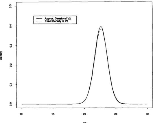
Thus, it is clear that the Bayesian results developed in this paper are reasonably useful for real data. All the conditional and extended predictions are somewhat comparable to those produced by the M L method. The adequacy of the approxima- tion for the conditional predictive density of V (2) given V (1) and Y is illustrated in Fig. 5 when the first column vector is treated as Vin the dental data set for girls alone.
J.C. Lee, EL. Hsu/Journal of Statistical Planning and Inference 64 (1997) 205-229 225 I ~ Approx. Ow~ly ot V2 Erect Domlty ol V2 I ei 0 | i 10 15 20 25 30 V2
* V is the dental measurement of the 1st gid.
Fig. 5. Comparison of exact and approximate density of V2 given VI and Y.
Finally, the computation involved is relatively simple and is conducted in the S-plus environment.
5. Concluding remarks
The Bayesian method presented in this paper provides an alternative way of dealing with the growth curve model when the serial covariance structure holds. The serial covariance structure is conceivably one of the most important dependence structures for this model. Although the results obtained so far are approximate in nature, they are at least comparable to those obtained by the ML method.
It is noted that the method presented in this paper provides an alternative way of constructing reliable regions for the parameters and the future values. Furthermore, the computations involved are relatively easy and should present no difficulty. It is therefore fair to say that the proposed method should be quite useful for practitioners in dealing with growth curve data.
226 J.C Lee, Y.L. Hsu/Journal of Statistical Planning and Inference 64 (1997) 205-229
Appendix
Theorem A.1. L e t X be distributed as xEv. I f Y IX = x ~ N (p, b E ® ( x A ) - 1 ) where
m x r
is m x m p.d., A is r x r p.d., b > O, then the distribution o f Y is given by
f ( Y ) = K(m, v,
r)lAIm/Ebm~/Zl~,l-r/zEb +
t r , ~ - l ( y _
t~)A(Y-
~u)']
mtv+r)/2,
(A.1)
where
~Fm(v[
2+ r) 1
K ( m , v, r) - I n-,~r/2. (A.2)
Proof. The joint distribution of Y and X is
(2~) ,~r/2
h-mr/2[yjl-r/2MIm/2 ym(v+r)/2 1f ( Y , X ) -- r ( m v / 2 ) 2 . ~ / 2 v ,_, ~., . .
+ g t r , ~ - ( Y - - p ) A ( Y - .
Next, integrating out X, we can obtain Eq. (A.1).
The density of Y as given in (A.1) is called the trace T distribution and will be denoted as
Y ~ T r ( p , A , b , ~ , - a , m ( v + r)). (A.4) It is noted that the distribution as given in (A.4) is one type of matrix generalization of the Students t-distribution and involves the trace of a matrix. When m or r is 1, then it will be reduced to the well-known multivariate T distribution. The first two moments of this distribution are given in the following theorem.
Theorem A.2. I f Y ,,~ Tr(~u,A, b, Z -1, m(v + r)), then
E ( Y ) = p (A.5a)
and
b
Cov(Y) - - - Z ® A - 1 (A.5b)
mv - 2
Proof. The p r o o f is completed by using the fact that
E ( Y ) = E x [ E ( Y I x ) ] and V a r ( Y ) = V a r x [ E ( Y I x ) ] + E x [ V a r ( Y ] x ) ] and X ,-~ ZZm~ implying E ( X - 1 ) = 1/(mv -- 2). []
J.C. Lee, Y.L. Hsu/Journal of Statistical Planning and Inference 64 (1997) 205-229 227
Theorem A.3. I f Y ~ T r ( p , A, b, X - 1, m(v + r)), then
b
U = b + t r , ~ - I(Y - p ) A ( Y - p)' "~ Beta(v1, v:), (A.6)
where vl = ½my and v2 = ½mr.
Proof. T h e mhth m o m e n t of U is EUmh = _f'(v 1 + v2)['(v 1 + mh)
F(Vl + v2 + mh)F(vO
which is the mhth m o m e n t of Beta(v1, v2). Since U is a b o u n d e d r a n d o m variable, its distribution is uniquely d e t e r m i n e d by its m o m e n t s .
T h e o r e m A.4. Let
{y(1)'] flit1)'] ( A l l A12~
Y = \ y ( 2 ) / ' fl = ~ ~ ( 2 ) J ' A = 2; -1 = \A21 A22/]
where yti),p(o are mi×r; Aij is mi×mj; ml + m z = m . I f Y . . ~ T r ( p , A , b , 2 -1, m(v + r)), then the marginal distribution of y ( 2 ) i s
y(2) ~ Tr(pt2),A, b, A22.1, m(v + r) - mlr) (A.7)
and the conditional distribution of y ( 1 ) [ y (2) is
Y(I)Iy(2) ~ Tr(/ta.z,A, c, All, m(v + r)), (A.8)
where
]~1.2 = ]~(1) + ,~12~221(I,r(2) - - ][/(2)),
c -= b + t r A 2 2 . 1 ( Y (2) - - ~ . / ( 2 ) ) A ( y ( 2 ) - - t / ( 2 ) ) , , (A.9)
A22.1 = A 2 2 - A z l A l 1 1 A 1 2 .
Proof. It can be s h o w n easily a n d hence is omitted. L e m m a A.1. For the generalized growth curve model,
t r C - 1(¥ _ X ~ A ) ( Y - X~A)'
= t r ( X ' C - 1X) [(X'C- 1X)- 1X'C- 1SC- ~X(X'C 1X)- 1 + (~ - ÷)AA'(~ -- ÷ ) ' ]
228 J.C. Lee, EL. Hsu/Journal of Statistical Planning and Inference 64 (1997) 205-229 w h e r e
S = Y [ ! - A ' ( A A ' ) - ' A ] Y ' ,
÷ = ( x ' c - l x ) lX'C-lVA'(AA') -1,
(A.11)
a n d Z is p x ( p - m) a n d o f r a n k p - m s u c h t h a t X ' Z = O.
It is noted that this is essentially (3.6) of Lee (1988c).
References
Chi, E.M., Reinsel, G.C, 1989. Models for longitudinal data with random effects and AR(1) errors. J. Amer. Statist. Assoc. 84, 452-459.
Elston, R.C., Grizzle, J.E., 1962. Estimation of time response curves and their confidence band. Biometrics 18, 148-159.
r e a m , T., 1975. A Bayesian approach to growth curves. Biometrika 62, 89-100. Geisser, S., 1970. Bayesian analysis of growth curves. Sankhya, Set. A 32, 53-64.
Geisser, S., 1980. Growth curve analysis. In: Krishnaiah, P.R., (Ed.), Handbook of Statistics, vol. 1. North- Holland, Amsterdam, pp. 89-115.
Geisser, S., 1981. Sample reuse procedures for prediction of the unobserved portion of a partially observed vector. Biometrika 68, 243-250.
Grizzle, J.E., Allen, D.M., 1969. Analysis of growth and dose response curves. Biometrics 25, 357-381. Jennrich, R.I., Schluchter, M.D., 1986. Unbalanced repeated measures models with structured covariance
matrices. Biometrics 42, 805 820.
Keramidas, E.M., Lee, J.C., 1990. Forecasting technological substitutions with concurrent short time series. J. Amer. Statist. Assoc. 85, 625-632.
Keramidas, E.M., Lee, J.C., 1995. Selection of a covariance structure for growth curves. Biometrical J. 37, 783-797.
Khatri, C.G., 1966. A note on a MANOVA model applied to problems in growth curves. Ann. Inst. Statist. Math. 18, 75 86.
Khatri, C.G., 1973. Testing some covariance structures under a growth curve model. J. Multivariate Anal. 3, 102 116.
Laitinen, K., 1978. Why is demand homogeneity so often rejected? Economics Lett. 1, 187 191. Lee, J.C., 1982. Classification of growth curves. In: Krishnaiah, P.R., Kanal, L.W. (Eds.), Handbook of
Statistics, vol. 2. North-Holland, Amsterdam, pp. 121-137.
Lee, J.C., 1988a. Growth curve model and technological forecasting. In: Matusita, K., (Ed.), Statistical Theory and Data Analysis, vol. 2. North-Holland, Amsterdam, pp. 369-378.
Lee, J.C., 1988b. Nested rotterdam model: applications to marketing research with special reference to telecommunications demand. Internat. J. Forecasting 4, 193-206.
Lee, J.C., 1988c. Prediction and estimation of growth curves with special covariance structures. J. Amer. Statist. Assoc. 83, 432-440.
Lee, J.C., 1991. Test and model selection for the general growth curve model. Biometrics 47, 147-159. Lee, J.C., Geisser, S., 1972. Growth curve prediction. Sankhya Set. A 34, 393-412.
Lee, J.C., Geisser, S., 1975. Applications of growth curve prediction. Sankhya Ser. A 37, 239-256. Lee, J.C., Geisser, S., 1996. On the prediction of growth curves In: Lee, J.C., Zellner, A., Johnson, W.O.
(Eds.), Modelling and Prediction Honoring Seymour Geisser. Springer, Berlin, 71 103.
Ljung, G.M., Box, G.E.P., 1980. Analysis of variance with autocorrelated observations. Scand. J. Statist. 7, 172-180.
Potthoff, R.F., Roy, S.N., 1964. A generalized multivariate analysis of variance model useful especially for growth curve problems. Biometrika 51,313-326.
J.C Lee, EL. Hsu/Journal of Statistical Planning and Inference 64 (1997) 205-229 229 Rao, C.R., 1965. The theory of least squares when the parameters are stochastic and its application to the
analysis of growth curves. Biometrika 52, 447-458.
Rao, C.R., 1966. Covariance adjustment and related problems in multivariate analysis. In: Krishnaiah, P.R., (Ed.), Multivariate Analysis, vol. 1. Academic Press, New York, pp. 87 103.
Rao, C.R., 1967. Least squares theory using an estimated dispersion matrix and its application to measurement of signals. In: LeCam, L.M., Neyman, J. (Eds.), Proc. 5th Berkeley Symp. Mathematical Statistics and Probability, vol. 1. University of California Press, Berkeley: pp. 355 372.
Rao, C.R., 1977. Prediction of future observations with special reference to linear models. In: Krishnaiah, P.R., (Ed.), Multivariate Analysis, vol. 4. Academic Press, New York, pp. 193-208.
Rao, C.R., 1984. Prediction of future observations in polynomial growth curve models. In: Proc. Indian Statistical Institute Golden Jubilee International Conference on Statistics: Applications and New Directions, Indian Statistical Institute, Calcutta, pp. 512-520.
Rao, C.R., 1987. Prediction of future observations in growth curve models. Statist. Sci. 2, 434-471. Williams, J.S., lzenman, A.J., 1981. A class of linear spectral models and analysis for the study of
longitudinal data. Technical Report, Dept. of Statistics, Colorado State University.
Zellner, A., Tiao, G.C., 1964. Bayesian analysis of the regression model with autocorrelated errors. J. Amer. Statist. Assoc. 59, 763 778.
Zerbe, G.O., 1979. Randomization analysis of the completely randomized design extended to growth and response curves. J. Amer. Statist. Assoc. 74, 215 221.