Proceedings of the 9th International Conference on Neural Information Processing (ICONIP'O2) , Vcll. 2 Lip0 Wang, Jagath C. Rajapakse, K u n h k o Fukushima, Soo-Young Lee, and Xin Yao (Editors)
RADIUS
MARGIN BOUNDS FOR
SUPPORT
VECTOR
MACHINES WITH THE RBF
KERNEL
Kai-Min Chung, Wei-Chun
Kao,
Tony Sun, Li-Lun Wang, and Chih-Jen Lin
National Taiwan University
.Department of Computer Science
Taipei 106, Taiwan
ABSTRACT Some early experiments on minimizing the right-hand side of (1.2)
An important approach for efficient support vector machine (SVM) model selection is to use differentiable bounds of the leave- one-out (loo) error. Past efforts focused on finding tight bounds of loo. However, their practical viability is still not very satisfactory.
In [5], it has been shown that radius margin bound gives good pre-
diction for LZSVM. In this paper, through the analyses why this bound performs well for LZSVM, we show that finding a bound whose minima are in a region with small loo values may be more important than its tightness. Based on this principle we propose modified radius margin bounds for L1-SVM where the original bound is only applicable to the hard-margin case. Our modifica- tion for L1-SVM achieves comparable performance to L:Z-SVM.
1. INTRODUCTION
Recently, support vector machines (SVM) [8] have been .a promis- ing tool for data classification. Its success depends on the tuning of several parameters which affect the generalization error. The error can be estimated by, for example, testing some data which are not used for training (e.g., cross validation) or by a bound from theo- retical derivation. The goal of this paper is to make one of these bounds, radius margin bound, a practical tool.
Given training vectors
xi
E E", i = 1,. . .
,
I , in two classes,and a vector y E R1 such that yi E (1, -l}, SVM solves:
(1.1)
1 T
min -w w
w,b 2
S.t. yi(wT+(zi)
+
b ) 2 1, i = 1,. .. ,
I ,where xi are mapped to a higher dimensional space by the func- tion
+.
Practically, we need only K ( z i , z j ) = + ( ~ , i ) ~ $ ( z j ) ,the kernel function. In this paper, we focus on the WBF kernel K ( z i , zj) = e-11"i--"J112/(2u2). The parameter (T is usually deter-
mined by an estimation of generalized error such as leave-one-out (loo) or cross validation. It was shown in [8] that the following radius margin bound holds
loo
5
4R211w112, (1.2)where loo is the number of loo errors, w is the solution of (l.l), and R is the radius of the smallest sphere containing all +(xi). It has been shown (e.g. [SI) that
R2
is the objective value ofmax
~ - , F K P
P
s.t. eT,B = 1 , O
5
pi,
z = 1, ..
.,
1. (1.3)are in [6].
However, (1.1) is not useful in practice. It may not be feasible if +(xi) are not linearly separable. In addition, a highly nonlinear $ may lead to overfitting. Thus, practically we solve either
1 - 1
where
ti
represents the training error and the parameter C adjusts the training error and the regularization term wTw/2. We refer to the two cases as L1-SVM and LZSVM, respectively. Note that for L2-SVM we use C/2 instead of C for easier analysis later. Then, if the RBF kernel is used, C and U are the two tunable parameters.Usually they are solved through dual problems. For L1-SVM, its
dual is 1
2 max e T a - - a T & a
S.t.
vTa
= 0,O5
ai5
C,i
= 1 , . . . , I , (1.5) where e is the vector of all ones and Q is an I x I matrix withQij = y i y j K ( z i , zj). For primal and dual optimal solutions,
(1
5)
The dual of L2-SVM is max a 1 I 2 C e T a-
-CY'(&
+
-)a s.t. y T a = O , O ~ a t , z = l,...
,1. (1.7) Unfortunately, for L1-SVM, the radius margin bound cannot be used as (1.2) does not hold. However, L2-SVM can be reduced to a form of (1.1) using lij and the ith training data as,
where e, is a zero vector of length 1 except the ith com- ponent is one. Then, (1.2) can be directly used so existing work on the radius margin bound focus on L2-SVM (e.g. [3, 71). Note thatR2
is now al20 different so we will denote the new bound asR2 llW)12, where R2 is the objective value of the following problem which has the same constraints as (1.3):
[,I
1 I
max 1
+
-
-p T ( ~
+
c)p.
(1.8)P C
[3] is the first to use the differentiability of (1.2) and develop optimization algorithms for finding optimal C and (T. This is much
Dataset banana image splice waveform tree L1 test err04 10.4(0.6) 1.9(1.0) 9.5(3.4) 10.2(3.2) 10.9(3.8)
(1.9) 55.9(10.0) 25.6(10.0) 15.5(8.1) 15.3(8.0) 17.0(-2.5) L2 test error 11.2(-1.4) 2.4(0.5) 9.5(3.3) 9.9(2.7) lOS(4.6)
Dataset banana image splice waveform m e
L1 test errox 10.4p.2) 1.9(3.9) 9.5(0.4) 10.2(1.4) 10.9(8.6) (1.9) 38.4(-2.9) 12.9(-2.9) 19.5(-2.4) 14.1(-2.5) 26.1(-10.0) L2 test errox 11.2(-0.0) 2.2Q.4) 10.1(2.1) 10.0(-0.0) lOS(9.7)
a2112211(2
ll.2(-0.9) 3.0(0.4) 10.2(10.0) 10.0(-0.6) 14.1(-1.4)at too small C or too large U . In the following we derive two other
bounds for LZSVM and through the comparison we show the RM bound for L2-SVM really possesses such mechanisms.
Remember the RM bound for L2-SVM is derived by consid- ering the hard margin SVM and using the following inequality (see, for example, Lemma 3 of [9]) : If in the leave-one-out proce- dure a support vector z p corresponding to a non-zero dual variable
aP
>
0 is recognized incorrectly, thenby changing L2-SVM to a hard-margin SVM formulation and A; is a subset of the convex hull by (21,
. . . ,
Z1}\{Zp}. Note that we slightly modify the derivation in [9] where the left-hand side of (2.1) is 1/(2D2). By the definition of A;,(2.3)
Since D is the diameter of the smallest sphere containing all (2.4) Therefore, if xp is recognized incorrectly, (2.1), (2.3), and (2.4) imply
a!:D4
2 1. Then, a p D 2 2 1 so withE,
aP = llG11*, we havep = l
Instead of using (2.4), from (2.2), we consider 2
llZi -
zjIl2
=+
Il4(.i) - 4(Zj)1I2.
WithIldJ(.i) - dJ(zj)1I2
I
D2 = 4R2,where R2 is the objective value of (1.3), we obtain a different bound
zoo
5
(4R2+
L),,G,l2. C (2.5) We can prove that under some conditions, (2.5) is a tighter bound:Theorem 1 I ~ u isfuced and R2
>
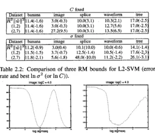
112, thenFor the five problems tested earlier, when U is fixed as values in
Table 2.1, R 2
>
1/2 holds.Some immediate comparisons between the two bounds %e as follows. When U is fixed, we can easily prove that lime-,, R2 =
limc+m R2 = limc+m(R2
+
v).
However, for small C R2&
but ( R 2+
y )
Y.
Therefore, when C is small, k211G112 overestimates the loo error. Interestingly this becomes a good property due to the following reason. From (2.1), the RM bound seriously overestimates the loo if ctP is large. This happens onlywhen C is not small. Thus, large a! happens only when C is large.
Therefore, the overestimation of loo at large C pushes the mini- mum to be at a smaller value of C . Therefore, we can think that R2 puts penalty at small C so the minimum of the RM bound may be pushed back to the correct position. In Table 2.2, we will see
(1.2) 11.4(-1.6) 3.0(-0.3) 10.0(3.1) 12.7(5.6) 17.0(-2.5
(2.7) 11.4(-1.6) 27.2(Y.5) 10.0(3.1) 13.5(6.5) 17.0(-2.5
3
'Dataset banana image splice waveform
R'~~C1~~'11.4(-1.6) 3.0(4.3) 10.0(3.1) 10.3(2.1) 17.0(-2.5
U fixed
(1.2) 11.5(-1.5) 3.7(-0.7) 12.5(-1.4) 10.5(-1.4) 17.6(-2;3
- Dataset banana image splice waveform
Rz~)2ir~~z11.2(-0.Y) 3.0(0.4) lO.l(lO.0) 10.0(-0.6) 14.1(-1.4
-
(2.7) 11.8(-2.1) 5.6(-1.8) 48.0(-10.0) 11.2(-2.2)
Figure 1: image dataset. The left one is the bound ( R 2
+
0.25/C)11W112, and the right one is the test error. For the bound, the minimum is at In U' = 9.5.that when U is fixed, (R2
+
v)llWl12
always retums a smallerc
thankz11Wl,112.
Next, we present another bound for L2-SVM. It motivates from the derivation of (1.9) which is a modified RM bound for L1-SVM. Remember that the original RM bound applies only to the hard-margin SVM. The derivation of (1.9) uses:
YP(fO(zP) - fP(ZP))
5
&PD2, (2.6)where z p is any support vector, a p is its corresponding dual vari- able, and fo and f p are the decision function trained, respectively,
on the whole set and after the point z p has been removed.
When there is an loo error, a p
>
0 so ypf0(zp) = 1 -t p .
Therefore, 0
5
-ypfP(zp)5
a p D 2 - 1+
tP
implies (1.1) For L2-SVM, (2.6) still holds under the same assum!ption. SoD 2 e T a
+
E:=,
.$i can be considered as a bound of loo for L2- SVM. With a = Cc and llu1112 = e T a for LZSVM, D 2 e T a+
E:=,
= D2eTa+
&eT,. Therefore, a new bound for L2 is: (2.7) In Table 2.2, it can be clearly seen that both new bounds are worse than the original RM bound, and (R2+
0.25/C)11W,112 which is a tighter bound than (2.5) is particularly bad.We observe that when C is fixed, the accuracy of using ( R2
+
0.5/C)(lW112 for waveform is not good because it obtains a too large U . Then, for( R 2
+
0.25/C)11~Z11~, it retums an even larger U so the error rate further increases. Especially for the problem image a very large 0 = 9.5 is obtainedIf U
-+
m, we can prove that R211G112 Mv,
( R 2+
y)llG[)'
Mv,
( E 2+
y ) l l G l 1 2 MF ,
where 11 and Ezare the number of data with yi = 1 and -1. Thus, smaller val- ues when U -+ m cause the bound ( R 2
+
0.25/C)11W112 to have minima at large 0. To confirm this in 1 we present the value of( R 2
+
0.25/C)llW112, using the problem image.Clearly there are two local minima where the lefi one is bet- ter but is not chosen. This seems to suggest that as R21(GllZ has
larger values when U -+ m, it can avoid that the global minimum
happens at a wrong place.
Besides, when 0 is fixed, the situation is also similar. The tighter the bound is, the worse the test accuracy is as the optimal
C
becomes too small. We can prove that changing the bound fromR2 to R2
+
9
and then R2+
F,
the optimal C decreases. Therefore, there is a benign overestimation for R when C is small. In summary, finding a bound whose minima are in a good region may be more important than its tightness. In addition, a good bound should avoid that minima happen at the boundary (i.e., too small or too large C and 0 2 ) .3. SOME HEURISTIC BOUNDS FOR L1-SVM Based on the experience in the previous section, we search for better radius margin bounds for L1-SVM which can replace the D2eTcu
+
E:=,
i$used in [5]. Our strategy is to consider that(R2
+
y ) l l W 1 1 2 for L2-SVM is the counterpart of D 2 e T a+
E',=,
EZ
for L1-SVM as they follow from the same derivation. Then, by investigating the difference betweenk2)(W112
and (R2+
y ) l l W 1 1 2 , we seek for the counterpart of
k21)W112
for L1-SVM.If we consider R' z R2
+
&,
k21)W112
is similar to(R2
+
&)llW112 = R 2 e T a+ Et=,
&
as11W112
= e T a and Q = Cc forL2-SVM. Thus, for L1-SVM,
R 2 e T a
+
2
ti
(3.1) i = lmay be a good bound. Now using (1.6),
CE",,,
llw1125
e T a , so another possibility is= e T a -
We will conduct experiments with these two new bounds later. Now we move on to another important issue: their differentiability. Then gradient-based methods can be used to find a local minimum. Unfortunately, in [4] we show that may not be differentiable.
Interestingly though e T a is not a differentiable function of
parameters, e T a
+
C
ti
is. The mainreason that
f
11w(12+
CE
&
= e T a - ! p T Q a is differentiable is that they are primal and dual objective functions at any given parameter set. Now both primal and dual solutions are functions of C and U in some unknown forms. So it may not be easy forthese bounds to be differentiable at parameters. However, for the primal or dual objective functions, using results of perturbation analysis of optimization problems, under some conditions, they are differentiable.
To have differentiability, we propose a further modification of
(3.2):
&
= (lw1(2+
2C(R2
+
~,,,,w,,,
+ 2 C k t i ) , (3.3) i = lwhere A is a positive constant close to one. As we discussed in Section 2, A/C can be thought as a penalty term for small C.
If we take A = 1, the main change from (3.2) is to replace e T a by a differentiable term.
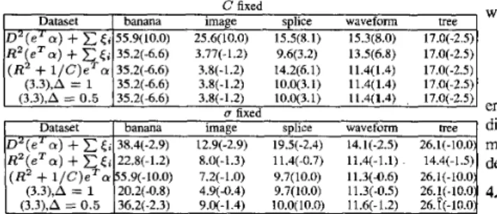
Table 3.1 presents a comparison of different bounds for L1- SVM: (1.9), (3.1), (3.2), and the differentiable bound (3.3) with A = 1 and A = 0.5. It can be clearly seen that bounds proposed in this section is better than (1.9).
Dataset banana image splice waveform tree
D 2 ( e " a )
+
C < i 55.9(10.0) 25.6(10.0) 15.5(8.1) 15.3(8.0) 17.0(-2.5)R 2 ( e T a )
+
<;
35.2(-6.6) 3.77(-1.2) 9.6(3.2) 13.5(6.8) 17.0(-2.5)IIXi
- " j0'
2u4
Table 3.1: Comparison of bounds for L1-SVM (error rate and and obtained In U' (or In C)).
4. EFFICIENT IMPLEMENTATION
( R 2
+
l / C ) S a 35.2(-6.6) 3.8(-1.2) 14.2(6.1) 11.4(1.4) 17.0(-2.5) (3.3),A = 0.5 352-6.6) 3.8(-1.2) 10.0(3.1) 11.4(1.4) , 17.0(-2.5)U fixed
(3.3),A = 1 35.2(-6.6) 3.8(-1.2) 10.0(3.1) 1 W 1 . 4 ) 17.0(-2.5) In [4], we show that the second derivatives of bounds consid- ered in this paper may not exist. Thus, Newton's method cannot be Dataset banana image splice waveform tree directly used. SO quasi-Newton and nonlinear conjugate gradient
D 2 ( e " a )
+
<,
38.4(-2.9) 12.9(-2.9) 19.X-2.4) 14.N-2.5) 26.1(-10.0) methods are the remaining major candidates. Following [7], we'R Z ( e T a )
+
ti 22W1.2) 8.0(-1.3) 11.4(-0.7) 114-1.1) 14.4(-1.3 decide to work on quasi-Newton methods.( R 2
+
l / C ) e T a 55.9(-10.0) 7.2(-1.0) 9.7(10.0) 11.3(-0.6) 26.1(-10.0) (3.3),A = 0.5 36.2(-2.3) 9.0(-1.4) lO.O(lO.0) 11.6(-1.2) 26.1(-10.0:(3.3),A = 1 20.2(-0.8) 4.9(-0.4) 9.7(10.0) 11.3(-0.5) 26.!(-10.0: 4.2. Quasi-Newton Methods
4.1. Differentiability of Bounds for L1-SVM
We have proposed to use (3.3) as the bound for L1-SVM. First, we denote it as f(C, a') and calculate its partial derivatives. For experiments in this section, we consider only A = 1.
The differentiability of both
R2
and llw11'+
2C x i = ,ti
re- lies on results of perturbation analysis of optimization problems. We consider Theorem 4.1 of [I] which states that for any opti- mization problem whose constraints are not related to parameters, if it has a unique minimizer, then the optimal value function is differentiable at parameters. Here, by the optimal value function we mean the optimal objective value as a function of parameters. However, though 1/211~11~+
CE:=,
is the objective function of the primal L1-SVM, the theorem does not apply as the optimalt
may not be unique, and constraints involve with the kemel param- eter a. Therefore, we look at the dual problem as at any optimal solution( 1.6) holds. For the RBF kemel, if no training data are at the same point (i.e., xi # x3), Q is positive definite. Then, (1.5) is a strictly convex quadratic programming problem, so the optimal a is unique under any given parameters. Without loss of general-ity from now on we assume 2% # x5. Then a remaining difficulty
is that constraints of the dual form of LI-SVM are related to C.
Therefore, we transform the dual to a problem whose constraints are independent of parameters: From (1.5), let (Y = CE:
1 - eTti min - c u ~ Q E - - - y T t i = 0,O
5
ti5
1 , i = 1,... ,Z.
Q 2 C s.t. (4.1) Then, 1-crTQa
-
e T a = C'(l&Qti-
e).
2 2 C (4.2)
Finally, we can apply Theorem 4.1 of [ 1 ] on (4.1) so
a($aT&(r
-
e T a ) 1= -(a*Qa
-
eTa).ac
CBecause the objective value of primal problem is the same as dual,
Similarly,
(4.5) by chain rules. An advantage is that the optimization prob- lem becomes unconstrained. Otherwise, C 2 0 and the property
u2 = (--U)' both cause problems. However, practically we still have to specify upper and lower bounds for In C and In U ' . Here,
we restrict them to be in [-lo, lo]. Once the optimization proce- dure has reached the boundary and still tends to move out, we stop it.
We consider the BFGS quasi-Newton method which has the following procedure: Assume x k is the current iterate and f(x) is the function to be minimized:
1 . Compute a search direction p = - H k V f ( x k ) .
2. Find xk+' = x k +Ap using a line search to ensure sufficient
3. Obtain Hk+1 by Hk+1 = ( I
-
$ ) H k ( I -g)
+
$,
where s = xk+'
-
x k and y = V f ( x k + ' ) -of(.')).
Here, Hk serves as the inverse of an approximate Hessian. The
f ( x k
+
Ap)I
f ( Z k )+
u l A v f ( x k ) T p , (4.6) where0<
u1<
1 isapositiveconstant. Sincep = - H k V f ( z k ) ,we need Hk to be positive definite to ensure that p is a descent direction. A good property of the BFGS formula is that Hk+l inherits the positive definiteness of Hk as long as y T s
>
0. The condition yTs>
0 is guaranteed to hold if the initial Hessian is positive definite (e.g. the identity) and the step size is determined by satisfying the second Wolfe condition:(4.7) decrease.
sufficient decrease by the line search usually means
Vf(Zk
+
Ap)1
u z V f ( z k ) T p ,where 0
<
u1<
U'<
1. Note that (4.6) is usually called the firstWolfe condition.
The main disadvantage of considering (4.7) is that the line search becomes more complicated. In addition, (4.7) involves the calculation of V f ( x k
+
Ap) so for each trial step size, a gradient evaluation is needed. Though V f ( d+
Ap) is easily computedonce f ( x k
+
Ap) is computed (as pointed out in [7]), this still contributes some additional cost.We consider an alternative approach to avoid the more com- plicated line search. If y T s
<
0, Hk is not updated. More specifi- cally, Hk+1 is determined by( I - $ ) H ~ ( I -
5 )
+
if yTs>
v,
otherwise, Hk+l = H k
{
where 7 is usually a small constant. Here, we simply use 7 = 0. Then the second Wolfe condition is not needed.
Regarding different trials of step size to ensure the sufficient decrease condition (4.6), we can simply find the largest value in a
set {yili = 0, 1, ...} such that (4.6) holds (y = 1/2 used in thispa- per). Also note that in early iterations, the search direction p may be a long vector so, using the initial X = 1, sometimes z"
+
p is far beyond the region considered. Thus, numerical instability may occur. Therefore, if zk+
Xp is outside the [-lo, 101 x [--lo, 101 region, we project it back by~ ( z t
+
xpZ) = "(-10, min(z$+
pi, 10)). We further avoid a too large step size by requiring the initial X to satisfy (IP(zk+
Xp) - zkll5
2. This reduces the chance of going to a wrong region in the beginning.4.3. Experiments
We use LIBSVM [2], which implements a decomposition method, to calculate 1 1 2 ~ ( 1 ~ , ll.rz1(12,
R 2 ,
and R 2 . The computational ex- periments for this section were done on a Pentium III-1C100 with 1024MB RAM. We keep all the default settings of LIBSVM ex- cept using a smaller stopping tolerance (default and increasing the cache size. It was pointed out in [7] that near the minimizer, llVfll is small so the error associated with findingl l ~ u 1 ( 1 ~ ,
113112, R2 or R2 may strongly affect the search direction. We have the same observation so decide to use a smaller stopping tolerance.We compare the quasi-Newton implementation for L1- and L2-SVM. For L1-SVM, we use (3.3) with A = 1. To demonstrate the viability for solving large problems, we include the problem ijcnnl which has 49,990 training and 91,701 testing samples in two classes. It is from the first problem of IJCNN challenge 2001. Note that we use the winner's transformation of raw data.
Tables 4.1 presents the result using an initial point (Cl, 0). We list the number of function and gradient evaluations, and the test accuracy. Results for L2-SVM are consistent with Table 1 of [7]. Note that the number of gradient evaluations is the same as the number of quasi-Newton iterations. Hence the average number of line searches in each iteration is very close to one. For problems image, splice, and tree, using L1-SVM, the algorithm reaches a point with In C = 10. At that point there are no bounded support vectors so we can set I n C to be the largest element of the dual variable (Y without affecting the model produced. Actually in final
iterations, there are already no bounded support vectors. We have not been able to develop early stopping criteria for such a situa- tion so decided to let the algorithm continue until it reaches the
boundary. Thus, for image and waveform, L1-SVM takes more iterations than L2-SVM. On the other hand, for splice, L2-SVM also reaches In C = 10. Overall except this difference, in terms of accuracy as well as computational cost, the bound for LI-SVM is competitive with that for L2-SVM.
For the large problem ijcnnl , RM bounds for both L1- and L2-SVM reach points with error rate around 2.91% and 2.17%, respectively. Unfortunately, this is a little worse than L.41% by
C
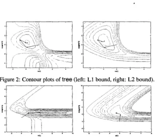
= 16 and u2 = 0.125 using cross validation. In addition, the number of support vectors is very different. There are about 17,000 support vectors comparing to 3370 when utilize cross validation. However, the total computational time is around 26,000 seconds (using the default as the stopping tolerance of L.IBSVM), much shorter than doing cross validation.To further compare bounds for L1- and L2-SVM, in Figure 2 and 3, we present contour plots of tree, and waveform, with search- ing paths on them. Note that in the L1 case of Figure 3, the final so-
lution is projected from (8.87, 1.38) to (1.25,1.38) because there is already no bounded support vectors.
Figure 2: Contour plots of tree (left: L1 bound, right: L2 bound).
Figure 3: Contour plots of waveform (left: L1 bound, right: L2 bound). The final solution for the L1 bound is projected from (8.87,1.38) to (1.25,1.38).
5. REFERENCES
[l] J. E Bonnans and A. Shapiro. Optimization problems with perturbations: a guided tour. SIAM Review, 40(2):228-264,
1998.
[2] C.-C. Chang and C.-J. Lin. LIBSVM: a library for support vector machines, 2001. Software available at http://www.csie.ntu.edu.tw/-cjlin/libsvm. [3] 0. Chapelle, V. Vapnik, 0. Bousquet, and S. Mukherjee.
Choosing multiple parameters for support vector machines.
Machine Learning, 46:13 1-159, 2002.
[4] K.-M. Chung, W.-C. Kao, T. Sun, L.-L. Wang, and C.-J. Lin. Radius margin bounds for support vector machines with the rbf kemel. Technical report, Department of Computer Sci- ence and Information Engineering, National Taiwan Univer- sity, 2002.
[5] K. Duan, S. S . Keerthi, and A. N. Poo. Evaluation of sim-
ple performance measures for tuning SVM hyperparameters.
Neurocomputing, 2002. To appear.
[6] T.-T. Friess, N. Cristianini, and C. Campbell. The kemel ada- tron algorithm: a fast and simple learning procedure for sup- port vector machines. In Proceedings of 15th Intl. Conf. Ma-
chine Learning. Morgan Kaufman Publishers, 1998. [7] S. S . Keerthi. Efficient tuning of SVM hyperparameters using
radiudmargin bound and iterative algorithms. IEEE Transac-
tions on Neural Networks, 2002. To appear.
[8] V. Vapnik. StatisticalLearning Theory. Wiley, New York, NY, 1998.
[9] V. Vapnik and 0. Chapelle. Bounds on error expectation for support vector machines. Neural Computation, 12(9):2013- 2036,2000.
image 96.24 97.03
tree 86.50 86.54 89.83
ijcnnl 9 9 97.09 97.83