利用樹狀結構探勘完整語意項目集
125
0
0
全文
(2) 致謝 精采的兩年研究所生活即將告一段落,回顧這一段時間的收穫與成長,內心 充滿許多的感動與感謝。這兩年的研究,首先最感謝的就是我的兩位指導教授洪 宗貝博士以及林浚瑋博士。因為兩位老師這兩年的耐心教導與鼓勵,讓我在研究 的道路上擁有許多的成長並且完成我的碩士論文,在此致上由衷的敬意與感謝。 其次,感謝我的碩士論文的口詴委員,高雄應用科技大學的潘正祥教授與台 南大學的李健興教授,謝謝他們能撥冗參加口詴會議並且對學生的碩士論文指導 修正並給予建設性及前曕性的建議,使我的論文更趨完整。 另外,感謝國誠學長在我的研究上給予相當多寶貴的建議與鼓勵,也讓我更 加了解做研究的精神與熱忱。感謝卓翰學長在我剛進入實驗室時給我很大的幫 助,讓我能夠在最短的時間內熟悉新的生活。感謝俊松學長的關心與鼓勵,雖然 學長已經離開實驗室進入職場工作,但還是時常在 MSN 上關心我的研究生活。 我也要感謝實驗室的學長姐、同學與學弟妹們,這兩年時間中對於我的鼓勵與幫 助,我的碩士生活也因為認識你們而更加美麗。 最後感謝我的家人以及高雄三一教會的所有朋友,謝謝你們對我的支持與禱 告,你們總在我心情沮喪時給予我滿滿的溫暖與鼓勵。這兩年來,受到許多人的 幫助,內心的感謝無法一一詳述,在此謹向所有關心、愛護以及鼓勵我的人,致 上我最深的謝意。. 林宗慶 謹誌 民國一百年七月.
(3) 利用樹狀結構探勘完整語意項目集 指導教授: 洪宗貝 博士 林浚瑋 博士 國立高雄大學資訊工程研究所. 學生: 林宗慶 國立高雄大學資訊工程研究所. 摘要. 隨著資訊科技快速的發展,電腦能夠處理以及儲存的資料量也大幅的提升, 如何從大量的資料當中找出隱藏的資訊以利於制定決策,是一個新的挑戰。近年 來,資料探勘技術經常被使用於從大型資料庫中發現有用的資訊與知識。在資料 探勘的研究領域中,關聯規則探勘是一個相當常見的討論議題。過去已經有許多 關於關聯規則探勘的演算法被提出,但是大部分的演算法都只能夠處理二元的資 料庫。然而,量化型的交易資料在現實的應用中是較為常見的。因此,許多關聯 規則探勘的研究加入模糊理論的概念來有效地處理量化型資料庫以及獲得語意 型式的關聯規則。本篇論文中,我們提出了三種演算法用來從量化型資料庫中探 勘出完整的模糊頻繁項目集,其分別是多重模糊頻繁樣式樹(MFFP-tree)、壓縮多 重 模 糊 頻 繁 樣 式 樹 (CMFFP-tree) 、 以 及 採 用 上 限 之 多 重 模 糊 頻 繁 樣 式 樹 I.
(4) (UBMFFP-tree)。在這三種演算法中,我們採用多重模糊區域的方式來表示該項 目數量,取代過去只利用單一模糊區域表示的方式,因此能夠獲得完整的模糊頻 繁項目集。另外本論文的實驗採用多個不同的資料庫來評估所提出的三種演算法 的效能。在效能的評估比較中,我們所提出的演算法顯示出在時間與空間的複雜 度上可以取得一個好的權衡。最後,我們也提出一種整合式的多重模糊頻繁樣式 樹(iMFFP-tree)演算法。此演算法可以將多棵來自不同資料庫的多重模糊頻繁樣 式樹整合成一棵完整的多重模糊頻繁樣式樹,以方便決策者可以直接從整合後的 樹中獲得全面性的關聯規則。. 關鍵字: 資料探勘、模糊資料探勘、頻繁樣式樹、多重模糊區域、樹狀結構。. II.
(5) Mining Complete Linguistic Itemsets Based on Tree Structures Advisors: Dr. Tzung-Pei Hong Dr. Chun-Wei Lin Department of Computer Science and Information Engineering National University of Kaohsiung. Student: Tsung-Ching Lin Department of Computer Science and Information Engineering National University of Kaohsiung. ABSTRACT. Information technology (IT) has recently progressed very rapidly, and the capacity to process and store data in databases has substantially grown. Extraction of implicit information from a lot of data to aid decision making has thus become a new challenge. Data mining technology is usually used to discover useful information and knowledge from large databases. In data-mining research areas, finding association rules is considered as one of the most common topics. In the past, many algorithms of. III.
(6) mining association rules have been proposed. Most of them focused on processing only binary variables in databases. Transactions with quantitative values are, however, commonly seen in real-world applications. The fuzzy-set theory is then used for efficiently handling them and deriving linguistic association rules. In this thesis, three algorithms for deriving complete fuzzy frequent itemsets from quantitative databases are proposed. They are multiple fuzzy FP-tree (MFFP-tree) algorithm, compressed multiple fuzzy FP-tree (CMFFP-tree) algorithm, and upper-bound multiple fuzzy FP-tree (UBMFFP-tree) algorithm, respectively. In all the three algorithms above, more than one fuzzy region, instead of only one region, are used to represent an item, thus being able to derive complete fuzzy frequent itemsets. Experiments are also made to compare the performance of the three proposed algorithms. The experimental results show that the proposed algorithms can achieve a good trade-off between execution time and tree complexity. In addition, we propose an integrated MFFP (iMFFP) tree algorithm for merging several individual MFFP trees into an integrated one. It can help derive global association rules from distributed databases.. Keywords: data mining, fuzzy data mining, frequent pattern tree, multiple regions, tree structure.. IV.
(7) Contents Chinese Abstract ....................................................................................................I English Abstract .................................................................................................. III CHAPTER 1 Introduction ................................................................................. 1 1.1 Background and Motivation ........................................................................................ 1 1.2 Thesis Organization ..................................................................................................... 4. CHAPTER 2 Review of Related Works............................................................ 5 2.1 Fuzzy-set Concepts ...................................................................................................... 5 2.2 Fuzzy Data Mining Approaches .................................................................................. 7 2.3 The F ............................................................................................................................ 9. CHAPTER 3 Multiple Fuzzy FP-tree Algorithm .......................................... 16 3.1 Notation...................................................................................................................... 16 3.2 The MFFP-tree Construction Algorithm ................................................................... 16 3.3 An Example of the MFFP-tree Construction Algorithm ........................................... 19 3.4 The MFFP-growth Mining Algorithm ....................................................................... 26 3.5 An Example of the MFFP-growth Mining Algorithm ............................................... 28. CHAPTER 4 Compressed Multiple Fuzzy FP-tree Algorithm .................... 34 4.1 Basic Concepts ........................................................................................................... 34 4.2 Notation...................................................................................................................... 37 4.3 The CMFFP-tree Construction Algorithm ................................................................. 37 4.4 An Example of the CMFFP-tree Construction Algorithm ......................................... 40 4.5 The CMFFP-mine Mining Algorithm ........................................................................ 47 4.6 An Example of the CMFFP-mine Algorithm ............................................................ 48. CHAPTER 5 Upper-Bound Multiple Fuzzy FP-tree Algorithm .................. 52 5.1 Notation...................................................................................................................... 52. V.
(8) 5.2 The UBMFFP-tree Construction Algorithm .............................................................. 53 5.3 An Example of the UBMFFP-tree Construction Algorithm ...................................... 55 5.4 The UBMFFP-growth Algorithm .............................................................................. 63 5.5 An Example of the UBMFFP-growth Algorithm ...................................................... 65. CHAPTER 6 Multiple Fuzzy FP-tree Merging Algorithm........................... 69 6.1 Notation...................................................................................................................... 70 6.2 The Multiple Fuzzy FP-tree Merging Algorithm....................................................... 70 6.3 An Example of the iMFFP-tree Algorithm ................................................................ 73. CHAPTER 7 Experiments and Discussion .................................................... 81 7.1 Experimental Results of the MFFP-tree Algorithm ................................................... 82 7.2 Experimental Results of the CMFFP-tree Algorithm ................................................ 87 7.3 Experimental Results of the UBMFFP-tree Algorithm ............................................. 94. CHAPTER 8 Conclusions and Future Works.............................................. 102 References ...................................................................................................... 105. VI.
(9) List of Figures Figure 2.1. The constructed FP tree ......................................................................................... 12 Figure 2.2. The conditional FP-tree for {h} ............................................................................. 13 Figure 2.3. The conditional FP-tree for {g} ............................................................................. 14 Figure 2.4. The conditional FP tree for {mg} .......................................................................... 15 Figure 3.1. Membership functions used in the example .......................................................... 20 Figure 3.2. The built Header_Table ......................................................................................... 22 Figure 3.3. The built MFFP tree after the first transaction has been processed ....................... 25 Figure 3.4. The built MFFP tree after the second transaction has been processed .................. 25 Figure 3.5. The finally constructed MFFP tree and its Header_Table ..................................... 26 Figure 3.6. The processed nodes {C.Middle} with its prefix paths ......................................... 29 Figure 3.7. The processed nodes {D.Low} with its corresponding paths ................................ 30 Figure 3.8. The conditional MFFP-tree of {D.Low} ............................................................... 31 Figure 3.9. The conditional MFFP-tree for {A.Middle, D.Low} ............................................. 31 Figure 3.10. The conditional MFFP-tree for {A.Middle, C.High, D.Low}.............................. 32 Figure 4.1. Membership functions used in this example ......................................................... 41 Figure 4.2. The built Header_Table ......................................................................................... 44 Figure 4.3. The CMFFP tree after the first transaction has been processed ............................ 46 Figure 4.4. The finally constructed CMFFP tree ..................................................................... 47 Figure 4.5. Tree nodes associated with {B.Low} ..................................................................... 49 Figure 5.1. Membership functions used in this example ......................................................... 56 Figure 5.2. The built Header_Table ......................................................................................... 59 Figure 5.3. The UBMFFP tree after the first transaction has been processed ......................... 61 Figure 5.4. The UBMFFP tree after the second transaction has been processed ..................... 62 Figure 5.5. The finally constructed UBMFFP tree .................................................................. 62 VII.
(10) Figure 5.6. The processed nodes {E.High} with its prefix paths ............................................. 66 Figure 5.7. The conditional UBMFFP-tree of {E.High} ......................................................... 67 Figure 6.1. Membership functions used in the example .......................................................... 74 Figure 6.2. The sub-MFFP tree of DB1 ................................................................................... 76 Figure 6.3. The sub-MFFP tree of DB2 ................................................................................... 77 Figure 6.4. All leaf nodes of the currently MFFP-tree............................................................. 77 Figure 6.5. Three branches of the currently sub-MFFP tree .................................................... 78 Figure 6.6. The iMFFP tree after merging the branch with fuzzy region {C.High} from the sub MFFP-tree of DB1 ........................................................................... 79 Figure 6.7. After merging the branch {C.High:0.4, D.Low:0.4, A.Middle:0.4, C.Middle:0.2}........................................................................................................ 79 Figure 6.8. After merging the branch {C.High:1.0, D.Low:1.0, C.Middle:0.4} ...................... 80 Figure 6.9. The finally merged MFFP-tree .............................................................................. 80 Figure 7.1. Comparison of the execution time obtained using the MF-Apriori and the MFFP-tree algorithm in the foodmart dataset ....................................................... 83 Figure 7.2. Comparison of the numbers of tree nodes obtained using the MFFP-tree algorithm in the foodmart dataset ......................................................................... 84 Figure 7.3. Comparison of the numbers of large itemsets obtained using the FFP-tree algorithm and the MFFP-tree algorithm in the foodmart dataset.......................... 85 Figure 7.4. Comparison of the execution time obtained using the MF-Apriori algorithm and the MFFP-tree algorithm in the BMS-POS dataset ....................... 86 Figure 7.5. Comparison of the numbers of tree nodes obtained using the MFFP-tree algorithm in the BMS-POS dataset ....................................................................... 86 Figure 7.6. Comparison of the numbers of large itemsets obtained using the FFP-tree algorithm and the MFFP-tree algorithm in BMS-POS dataset ............................. 87 Figure 7.7. Comparison of the execution time obtained using the MF-Apriori VIII.
(11) algorithm and the CMFFP-tree algorithm in the foodmart dataset ....................... 88 Figure 7.8. Comparison of the execution time obtained using the MFFP-tree algorithm and the CMFFP-tree algorithm in the foodmart dataset ....................................... 89 Figure 7.9. Comparison of the numbers of tree nodes for fuzzy 2-regions obtained using the MFFP-tree algorithm and the CMFFP-tree algorithm in the foodmart dataset .................................................................................................... 90 Figure 7.10. Comparison of the numbers of tree nodes for fuzzy 3-regions obtained using the MFFP-tree algorithm and the CMFFP-tree algorithm in the foodmart dataset .................................................................................................... 90 Figure 7.11. Comparison of the execution time for fuzzy 2-regions obtained using the MFFP-tree algorithm and the CMFFP-tree algorithm in the chess dataset .......... 91 Figure 7.12. Comparison of the numbers of tree nodes for fuzzy 2-regions obtained using the MFFP-tree algorithm and the CMFFP-tree algorithm in the chess dataset .......................................................................................................... 91 Figure 7.13. Comparison of the execution time for fuzzy 3-regions obtained using the MFFP-tree algorithm and the CMFFP-tree algorithm in the chess dataset .......... 93 Figure 7.14. Comparison of the numbers of tree nodes for fuzzy 3-regions obtained using the MFFP- tree algorithm and the CMFFP-tree algorithm in the chess dataset .......................................................................................................... 93 Figure 7.15. Comparison of execution time for fuzzy 2-regions obtained using MF-Apriori algorithm and UBMFFP-tree algorithm in foodmart dataset ............ 94 Figure 7.16. Comparison of execution time for fuzzy 2-regions obtained using the proposed three fuzzy FP-tree algorithms in the foodmart dataset ........................ 95 Figure 7.17. Comparison of the numbers of tree nodes for fuzzy 2-regions obtained using the proposed three fuzzy FP-tree algorithms in the foodmart dataset ......... 95 Figure 7.18. Comparison of the execution time for fuzzy 3-regions obtained using the IX.
(12) MF-Apriori algorithm and the UBMFFP-tree algorithm in the foodmart dataset.................................................................................................................... 96 Figure 7.19. Comparison of the execution time for fuzzy 3-regions obtained using the proposed three fuzzy FP-tree algorithms in the foodmart dataset ........................ 97 Figure 7.20. Comparison of the numbers of tree nodes for fuzzy 3-regions obtained using the proposed three fuzzy FP-tree algorithms in the foodmart dataset ......... 97 Figure 7.21. Comparison of the execution time for fuzzy 2-regions obtained using the proposed three fuzzy FP-tree algorithms in the mushroom dataset ...................... 98 Figure 7.22. Comparison of the numbers of tree nodes for fuzzy 2-regions obtained using the proposed three fuzzy FP-tree algorithms in the mushroom dataset.................................................................................................................... 99 Figure 7.23. Comparison of the execution time for fuzzy 3-regions obtained using the proposed three fuzzy FP-tree algorithms in the mushroom dataset .................... 100 Figure 7.24. Comparison of the numbers of tree nodes for fuzzy 3-regions obtained using the proposed three fuzzy FP-tree algorithms in the mushroom dataset.................................................................................................................. 100. X.
(13) List of Tables Table 2.1. Five transactions in database .................................................................................. 10 Table 2.2. All items with their counts ...................................................................................... 11 Table 2.3. The updated transactions in database ...................................................................... 11 Table 3.1. Six transactions with purchased items and its quantitative values ......................... 19 Table 3.2. Fuzzy sets transformed from Table 3.1 ................................................................... 20 Table 3.3. Counts of fuzzy regions .......................................................................................... 21 Table 3.4. Counts of fuzzy frequent regions ............................................................................ 22 Table 3.5. The remaining fuzzy regions .................................................................................. 23 Table 3.6. The updated transactions for constructing the MFFP tree ...................................... 23 Table 3.7. The derived fuzzy frequent itemsets of {D.Low} ................................................... 33 Table 3.8. All derived fuzzy frequent itemsets from the MFFP tree ....................................... 33 Table 4.1. Six transactions with purchased items and its quantitative values ......................... 40 Table 4.2. Fuzzy sets transformed from Table 4.1 ................................................................... 42 Table 4.3. Counts of fuzzy regions .......................................................................................... 42 Table 4.4. The fuzzy regions, its counts and its occurrence frequencies ................................. 43 Table 4.5. The updated transactions for constructing the CMFFP tree ................................... 44 Table 4.6. All derived fuzzy itemsets from the CMFFP tree ................................................... 50 Table 4.7. All derived fuzzy frequent itemsets from the CMFFP tree ..................................... 51 Table 5.1. Eight transactions with purchased items and its quantitative values ...................... 55 Table 5.2. Fuzzy sets transformed from Table 5.1 ................................................................... 57 Table 5.3. Counts of fuzzy regions .......................................................................................... 57 Table 5.4. The fuzzy regions, its counts and its occurrence frequencies ................................. 58 Table 5.5. The updated transactions for constructing the UBMFFP tree................................. 59 Table 5.6. The final set of candidate fuzzy itemsets ................................................................ 68 XI.
(14) Table 5.7. All derived fuzzy frequent itemsets from the UBMFFP tree .................................. 68 Table 6.1. Two quantitative databases in the example ............................................................. 73 Table 6.2. Fuzzy sets transformed from Table 6.1 ................................................................... 75 Table 6.3. Counts of fuzzy regions (fuzzy frequent itemsets) ................................................. 76. XII.
(15) CHAPTER 1 Introduction 1.1 Background and Motivation As information technology (IT) has rapidly progressed, data mining becomes a useful tool to help mangers make efficient decision. Depending on a variety of knowledge desired, data mining approaches can be divided into association rules [2, 4], classification [17, 38], clustering [22, 27], and sequential patterns [3, 36], among others. Among them, mining association rules from databases is especially common seen in data mining research [2, 6, 8, 32-33].. Many algorithms for mining association rules from databases have been proposed over the years. Most of them are based on the Apriori algorithm [2] to generate and test the candidate itemsets level by level. Thus, high computational cost is required for iteratively scanning databases in the Apriori approach. Han et al. then proposed the frequent-pattern-tree (FP-tree) structure for efficiently mining association rules without generating candidate itemsets [13]. In the FP-tree structure, an original database is compressed into a tree structure tuple by tuple for only frequent (also called large) items. A recursive mining procedure called FP-growth is then executed for mining frequent itemsets from the constructed FP-tree structure. 1.
(16) In the past, mining association rules processed data with binary attributes to represent the occurrence of items. Transactions with quantitative values are, however, commonly seen in real-world applications. The quantitative data is, however, hard to represent by traditional crisp sets. The fuzzy set theory [43] has been applied for efficiently handling the quantitative data due to its simplicity and similarity to human reasoning. Several fuzzy data mining algorithms have been designed for handling quantitative data [14-15], which use the Apriori algorithm to generate-and-test fuzzy frequent itemsets level-by-level. Membership functions are used to transform each quantitative value into linguistic terms according to fuzzy-set theory. The cardinality of each linguistic term is then calculated for all transaction data for the subsequent mining process to derive the fuzzy association rules [24-26, 31].. The above approaches, however, considered that each term uses only the linguistic term with the maximum cardinality in later processes; the number of fuzzy regions processed is thus equal to the number of original items, which reduces processing time. Considering the multiple regions of an item to form the complete fuzzy association rules, however, is more reasonable in real-world applications than only considering a single linguistic term with the maximum cardinality to represent fuzzy association rules. In this thesis, a framework for efficiently mining the complete fuzzy frequent itemsets from quantitative databases is thus proposed. Each item may. 2.
(17) be represented by multiple linguistic terms in subsequent processes, thus deriving more complete fuzzy frequent itemsets. Three different algorithms called multiple fuzzy FP-tree. (MFFP-tree). algorithm,. compressed multiple fuzzy FP-tree. (CMFFP-tree) algorithm, and upper-bound multiple fuzzy frequent pattern tree (UBMFFP-tree) algorithm are then respectively designed for constructing its own tree structures in this thesis. In mining process for deriving fuzzy frequent itemsets, the fuzzy regions transformed from the same item cannot be joined forming the fuzzy frequent itemsets due to the meaningless. In the experiments, the proposed three algorithms are then consequentially compared to show the performance in different support thresholds among different databases. The execution time and numbers of tree nodes are then evaluated for revealing that our proposed algorithms can thus achieve a good trade-off between time and tree complexity.. Since data mining can reveal the relationships among the purchased items, it can be thus considered as a useful tool for decision making. The above three approaches, however, only consider one database in whole mining processing. In real-world applications, however, multiple databases may exist in different areas or branches of a parent company. It is an important research issue to integrate individual information into one for making the comprehensive and significant decision for a parent company. In this thesis, we also propose an integrated MFFP (iMFFP) tree merging algorithm. 3.
(18) for merging several sub-MFFP trees into one. Each branch only constructs their own specified sub-MFFP tree for sorting the fuzzy frequent 1-itemsets in the parent company. After that, the branches in sub-MFFP tree are then efficiently extracted to integrate the other sub-MFFP tree in a sequence, thus forming an integrated MFFP (iMFFP) tree.. 1.2 Thesis Organization The remaining parts of this thesis are organized as follows. Some related researches including, fuzzy-set concepts, fuzzy data mining approaches, and the FP-growth algorithm are shortly reviewed in Chapter 2. Three proposed algorithms are respectively described in Chapters 3, 4 and 5 with their examples. The proposed integrated MFFP (iMFFP) tree merging algorithm is indicated in Chapter 6. Experiments are mentioned in Chapter 7. Conclusions and future works are stated in Chapter 8.. 4.
(19) CHAPTER 2 Review of Related Works In this chapter, we review some related researches about this thesis. They are fuzzy-set concepts, fuzzy data mining approaches, and the FP-growth algorithm.. 2.1 Fuzzy-set Concepts In 1965, Zadeh proposed fuzzy sets and introduced membership function as a method of quantitative description [43]. The fuzzy sets with their linguistic modes of reasoning are more natural to human beings, rather than the binary logic of 0 and 1 in computer science. The fuzzy set theory extends this concept by defining partial memberships, which can take values ranging from 0 to 1. A membership function is formally defined as: [20, 43]:. u A : X 0, 1 , where X refers to the universal set for a specific problem. Assume that A and B are two fuzzy sets with membership functions uA(x) and uB(x), respectively, the following common fuzzy operators can be defined [43].. (1) Intersection operator:. 5.
(20) u AB ( x) u A ( x) u B ( x) where τ is a t-norm operator. That is, τ is a function of 0, 1* 0, 1 0, 1 and must satisfy the following conditions for each a, b, c 0, 1 : i. a 1 a; ii. a b b a; iii. a b c d if a c, b d ; iv. a b c a (b c) (a b) c. Two instances of a t-norm operator for a τ b are min(a, b) and a ∗ b. (2) Union operator:. u AB ( x) u A ( x) u B ( x) , where ρ is an s-norm operator. That is, ρ is a function of 0, 1* 0, 1 0, 1 and must satisfy the following conditions for each a, b, c 0, 1 : i. a 0 a; ii. a b b a; iii. a b c d if a c, b d ; iv. a b c a (b c) (a b) c. Two instances of an s-norm operator for a ρ b are max(a, b) and a + b - a ∗ b. (3) cut operator:. A ( x) {x X | u A ( x) }. 6. ,.
(21) where A is an α-cut of fuzzy set A. Aα thus contains all the elements in the universal set X that has membership grades in A greater than or equal to the specified value of α. These fuzzy operators are used in the proposed fuzzy FP-tree mining algorithms to derive fuzzy frequent itemsets.. 2.2 Fuzzy Data Mining Approaches Deriving association rules from transaction databases is most commonly seen in data mining [2, 6, 8, 32-33]. It discovers relationships among purchased items such that the presence of certain items in a transaction tends to imply the presence of certain other items. Traditional association rules algorithms treat items as binary variables in databases, which consider whether an item is bought in databases or not. Transactions with quantitative values are, however, also commonly seen in real-world applications. In these years, the fuzzy set theory [43] has been used frequently in intelligent systems because of its simplicity and similarity to human reasoning. Linguistic terms are easily implemented using fuzzy sets, as fuzzy set theory is concerned with quantifying and reasoning using natural language. Several fuzzy mining approaches have been proposed for discovering fuzzy association rules from transaction data with quantitative values. Kuok et al. proposed a fuzzy mining approach for handling numerical data in databases and deriving fuzzy association. 7.
(22) rules [21]. Hong et al. proposed fuzzy mining algorithms for discovering fuzzy rules from quantitative transaction data [14-15]. Papadimitriou et al. proposed an approach based on FP-trees for finding fuzzy association rules [31]. In this approach, a fuzzy region in a transaction is removed if its transformed fuzzy value is smaller than the threshold. That is, it only keeps the local frequent fuzzy 1-itemsets in each transaction, thus used for later mining process. However, the expression of fuzzy patterns is straight without using any fuzzy operations to form the desired rules. This procedure thus makes the mined fuzzy rules a little difficult to understand. Lin et al. thus proposed three fuzzy data mining algorithms [24-26] to efficiently mine the fuzzy frequent itemsets from quantitative databases, which extended the FP-tree mining process for constructing its suitable tree structures. These algorithms transform quantitative values in transactions into linguistic terms based on Hong et al.’s approach [14-15] that only keeping the linguistic term with the maximum cardinality. They make the number of fuzzy regions processed equal to the number of original items, which reduces the processing time. The fuzzy frequent itemsets, represented by linguistic terms, are then derived from the constructed tree structures. Many mining methods for finding fuzzy association rules have been also proposed [5, 9, 16, 18, 34, 37, 41].. 8.
(23) 2.3 The Frequent Pattern Tree Frequent pattern mining is one of the most important data mining problems. The initial solution for the problem of association rule mining was given by Agrawal et al. [2] in the form of Apriori algorithm which is based on level-wise candidate set generation and test methodology. However, because the size of the database can be very large, it is very costly to repeatedly scan the database to count supports for candidate itemsets. The limitations of Apriori algorithm are overcome by an innovative approach proposed the frequent pattern (FP) tree structure and the FP-growth algorithm by Han et al. [13].. Their approach can efficiently mine. frequent itemsets without the generation of candidate itemsets, and it scans the original transaction database only twice. The mining algorithm consists of two phases; the first constructs an FP-tree structure and the second recursively mines the frequent itemsets from the structure. The details of two phases for the FP-growth algorithm [13] are respectively described below.. 2.3.1 Construction of FP-tree The FP-tree is a compact tree structure storing frequent items from databases. The Header_Table is also built as an index table, thus keeping not only the frequent items but also its occurrence frequencies. Each item in Header_Table points to its first occurrence in the tree through a node-link. Nodes with the same item in the tree are 9.
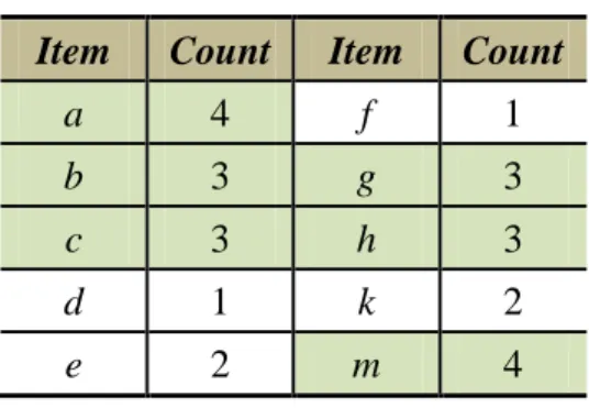
(24) also connected in a sequence. It can fast trace the same items in the tree, for efficiently generating the frequent itemsets. The construction of FP tree requires two database scans. The first database scan is to identify all frequent (or large) items. In the second database scan, frequent items within transactions are sorted in descending order according to the occurrence frequencies of items. The construction process is then executed tuple by tuple, from the first transaction to the last one. After all transactions in databases are processed, the FP tree is completely constructed. Here, an example shown in Table 2.1 is used to illustrate the construction process. The minimum support threshold is set at 50%.. Table 2.1. Five transactions in database TID. Items. 1. a, b, e. f, g, h, m. 2. a, c, g, k, m. 3. a, b, d, h. 4. a, c, e, g, m. 5. b, c, k, h, m. The database in Table 2.1 is then scanned to calculate the occurrence frequencies (count) of items and check whether the count of items is larger than or equal to the minimum count, which is 5*50% (= 2.5). The results are shown in Table 2.2, in which the large items are marked in green color.. 10.
(25) Table 2.2. All items with their counts Item. Count. Item. Count. a. 4. f. 1. b. 3. g. 3. c. 3. h. 3. d. 1. k. 2. e. 2. m. 4. As the results in Table 2.2, the infrequent items are eliminated from the original database in Table 2.1. The remaining frequent items are sorted by their count in a descending order. The updated transactions in database are shown in Table 2.3.. Table 2.3. The updated transactions in database TID. Items. 001. a, m, b, g, h,. 002. a, m, c, g. 003. a, b, h. 004. a, m, c, g. 005. m, b, c, h. The updated transactions in Table 2.3 are used to construct an FP tree tuple by tuple from the first transaction to the last one. There are two cases to be checked for constructing the FP tree. For the processed transaction, first, the order of items is exactly matched to the tree path; the count of each node in the path can be incremented by 1. In the second case, a new tree path is then built since the processed. 11.
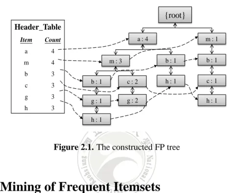
(26) transaction is not matched to existing tree path; the count of node in newly built path is then set at 1. After all transactions are processed, the Header_Table and the FP tree are shown in Figure 2.1.. {root} Header_Table Item. Count. a. 4. m. 4. b. 3. c. 3. g. 3. h. 3. a:4 m:3. b:1. c:2. g:1. g:2. m:1 b:1. b:1. h:1. c:1 h:1. h:1. Figure 2.1. The constructed FP tree. 2.3.2 Mining of Frequent Itemsets After the construction of an FP tree, the complete frequent itemsets can be discovered by the FP-growth mining approach [11]. The FP-growth algorithm is more efficient and scalable rather than the Apriori algorithm [2] since the candidate itemsets is unnecessary to generate level-by-level. The FP-growth algorithm is recursively mine frequent itemsets one by one and bottom-up from the Header_Table. A conditional FP tree is generated for each frequent item, and the frequent itemsets with the processed item are recursively derived from the tree. Below, the constructed FP tree in Figure 2.1 is used to illustrate the FP-growth procedure.. 12.
(27) The frequent items from the Header_Table in Figure 2.1 are processed one by one from bottom to top. In this example, item {h} is first processed. Three prefix paths for item {h} are {a: 4, m: 3, b: 1, g: 1, h: 1}, {a: 4, b: 1, h: 1} and {m: 1, b: 1, c: 1, h: 1}. The counts of all nodes in the first path are then updated as 1 since they only appear once with item {h:1} in the branch. Similarly, the counts of all nodes in the second and third path are also updated in the same way. Thus, three converted prefix paths are {a: 1, m: 1, b: 1, g: 1, h: 1}, {a: 1, b: 1, h: 1} and {m: 1, b: 1, c: 1, h: 1}. The counts of the rest items in three prefix paths are then summed together to check whether the counts of items are larger than or equal to the minimum count, which is 2.5. In this example, only item {b} is a large item with item{h: 3}. The conditional FP tree for item {h} is shown in Figure 2.2, and the frequent itemsets can be generated for item {h} are {h: 3} and {bh: 3}.. {root} a:4. m:1 h:3. m:3. b:1. b:1. b:1. h:1. c:2. b:3. Conditional FP-tree with {h} g:1. h:1. h:1. Prefix path with {h}. Figure 2.2. The conditional FP-tree for {h} 13.
(28) Next, item {g} is processed. There are two converted prefix paths {a: 1, m: 1, b: 1, g: 1} and {a: 2, m: 2, c: 2, g: 2} for item {g}. The counts of items in the paths are summed together, and the counts of items {a} and {m} are larger than the minimum count. The set of large items for the conditional FP tree of item {g} are thus {a, m}. The conditional FP-tree for item {g} is shown in Figure 2.3.. {root} a:3. g:3. m:3. a:3. b:1. c:2. g:1. g:2. m:3. Conditional FP-tree with {g}. Prefix path with {g}. Figure 2.3. The conditional FP-tree for {g}. The frequent patterns with item {g} can be generated as {g: 3}, {mg: 3} and {ag: 3}. A conditional FP tree is then recursively constructed in the sequence of {mg: 3} and {ag: 3}. The prefix path for {mg: 3} is {a: 3}. The conditional FP tree for itemset {mg} is shown in Figure 2.4. The large itemsets with {mg} are {mg: 3} and {amg: 3}. Because of there is no any prefix paths of itemset {amg}, the recursive procedure of itemset {mg} is then completed.. 14.
(29) g:3 mg : 3 a:3. a:3 m:3. Conditional FP-tree with {mg}. Conditional FP-tree with {g}. Figure 2.4. The conditional FP tree for {mg}. After processed itemset {mg}, the recursive procedure of itemset {ag} is then processed. Since there is no any prefix paths of itemset {ag}, the recursive process of item {g} is then completed. The derived frequent itemsets for item {g} are {g: 3}, {mg: 3}, {ag: 3} and {agm: 3}. The above recursive procedure is repeated for other items in the Header_Table until all items are processed. Several other algorithms based on the FP-tree structure have been proposed. Qiu et al. proposed the QFP-growth mining approach to mine association rules [40]. Ezeife et al. constructed a generalized FP tree, which stores all frequent and infrequent items, for incremental mining without rescanning databases [10]. Many related researches are still in progress for efficiently discovering the desired information [1, 11, 23, 28, 35, 39, 42].. 15.
(30) CHAPTER 3 Multiple Fuzzy FP-tree Algorithm In this chapter, the multiple fuzzy FP-tree (abbreviated as MFFP-tree) algorithm is proposed to keep fuzzy frequent regions whether they are generated from the same item or not. The MFFP-tree structure is used to efficiently handle quantitative data with multiple fuzzy regions of an item (term). The notation used in the proposed MFFP-tree algorithm is shown below.. 3.1 Notation D. the original quantitative database;. n. the number of transactions in D;. T. the i-th transaction in D, 1 i n ;. m Ij. the number of items in D; the j-th item, 1 j m ;. hj. the number of fuzzy regions for Ij;. Rjl. the l-th fuzzy region of Ij, 1 l h j ;. vij. the quantitative value of Ij in T;. fijl. the membership value of vij in region Rjl;. countjl s. the count of the fuzzy region Rjl in D; the predefined minimum support threshold.. 3.2 The MFFP-tree Construction Algorithm INPUT: A quantitative database consisting of n transactions, a set of membership 16.
(31) functions, and a predefined minimum support threshold s. OUTPUT: A multiple fuzzy FP tree (MFFP tree). STEP 1: Transform quantitative value vij of each item Ij in the i-th transaction into a fuzzy set fij represented as (fij1/Rj1 + fij2/Rj2 + …+ fijh/Rjh) using the given membership functions, where h is the number of fuzzy regions for Ij, Rjl is the l-th fuzzy region of Ij, 1 l h , and fijl is vij’s fuzzy membership value in region Rjl. Note that fijl/Rjl means that the membership value of region Rjl is fijl. STEP 2: Calculate the scalar cardinality countjl of each fuzzy region Rjl in the transactions as: n. count jl f ijl . i 1. STEP 3: Check whether the value countjl of the fuzzy region Rjl is larger than or equal to the predefined minimum count n*s. If the count of a fuzzy region Rjl is equal to or greater than the minimum count, it can be treated as a fuzzy frequent itemset and put it in the set of L1. That is: L1 = {Rjl | countjl n*s, 1 j m}. STEP 4: Build the Header_Table by sorting the fuzzy regions (fuzzy frequent itemsets) in L1 in descending order of their fuzzy values. STEP 5: Remove the fuzzy regions of the items not existing in L1 from the. 17.
(32) transactions of the transformed database. STEP 6: Sort the remaining fuzzy regions in descending order of their fuzzy values in each transaction. STEP 7: Initially set the root node of the MFFP tree as {root}. STEP 8: Insert the transactions of the transformed database into the MFFP tree tuple by tuple. The following two cases may exist. Substep 8-1: If a fuzzy region Rjl in a transaction is at the corresponding branch of the MFFP tree, add the fuzzy value fijl of Rjl in the processed transaction to the node of Rjl in the branch. Substep 8-2: Otherwise, add a node of Rjl at the end of the corresponding branch, set the count of the node as the fuzzy value fijl of Rjl, and connect the node of Rjl in the last branch with the current node as a sequence. If there is no such branch with the node of Rjl, insert a node-link from the entry of Rjl in Header_Table to the added node.. In STEP 8, a corresponding branch is the branch built in the MFFP tree according to sorted fuzzy regions in descending order of their fuzzy values in the transformed transactions. After STEP 8, the final MFFP tree is thus built.. 18.
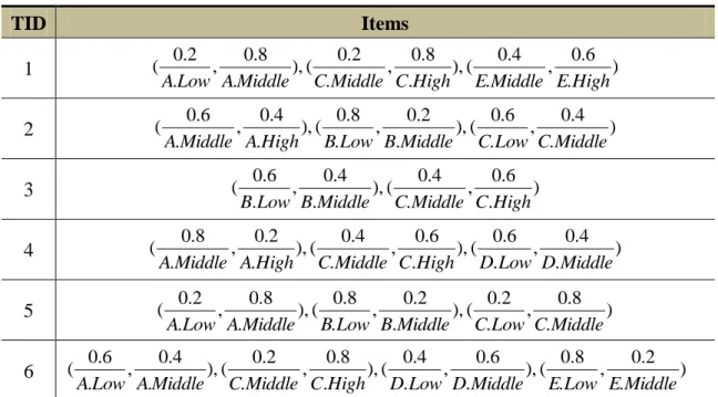
(33) 3.3 An Example of the MFFP-tree Construction Algorithm Below, an example is given to illustrate how to construct a MFFP tree from quantitative transaction data, which is shown in Table 3.1. It consists of 6 transactions and 5 items, denoted A to E. The minimum support threshold s is initially set to 30%.. Table 3.1. Six transactions with purchased items and its quantitative values TID. Items. 1. (A:5) (C:10) (D:2) (E:9). 2. (A:8) (B:2) (C:3). 3. (B:3) (C:9). 4. (A:7) (C:9) (D:3). 5. (A:5) (B:2) (C:4). 6. (A:3) (C:11) (D:2) (E:2). Assume that the fuzzy membership functions are the same for all items shown in Figure 3.1. In this example, amounts are represented by three fuzzy regions: {Low}, {Middle}, and {High}. Thus, three fuzzy membership values are produced for each item in a transaction according to the predefined membership functions in Figure 3.1. Note that the proposed approach also works when the membership functions of the amounts for the items are not the same.. 19.
(34) Low. Middle. High. Membership value. 1. 0. 1. 6. 11. Amount. Figure 3.1. Membership functions used in the example. The MFFP tree for this example is thus constructed using the proposed approach as follows. STEP 1: The quantitative values of the items in the transactions are represented as fuzzy sets using the membership functions shown in Figure 3.1. Take item {A} in transaction 1 as an example to illustrate the procedure. The amount “5” of {A} can be converted into the fuzzy set (. 0.2 0.8 ) by the membership functions in , A.Low A.Middle. Figure 3.1. This step is repeated for the other items in Table 3.1, and the results are shown in Table 3.2.. Table 3.2. Fuzzy sets transformed from Table 3.1 TID 1 2. Items (. 0.2 0.8 0.2 0.8 0.8 0.2 0.4 0.6 , ), ( , ), ( , ), ( , ) A.Low A.Middle C.Middle C.High D.Low D.Middle E.Middle E.High. (. 0.6 0.4 0.8 0.2 0.6 0.4 , ), ( , ), ( , ) A.Middle A.High B.Low B.Middle C.Low C.Middle. 20.
(35) (. 3 (. 4. 0.8 0.2 0.4 0.6 0.6 0.4 , ), ( , ), ( , ) A.Middle A.High C.Middle C.High D.Low D.Middle (. 5 (. 6. 0.6 0.4 0.4 0.6 , ), ( , ) B.Low B.Middle C.Middle C.High. 0.2 0.8 0.8 0.2 0.4 0.6 , ), ( , ), ( , ) A.Low A.Middle B.Low B.Middle C.Low C.Middle. 0.6 0.4 1.0 0.8 0.2 0.8 0.2 , ), ( ), ( , ), ( , ) A.Low A.Middle C.High D.Low D.Middle E.Low E.Middle. STEP 2: The scalar cardinality of each fuzzy region in transactions is calculated as the count value. Take the fuzzy region {A.Low} as an example to explain the procedure. {A.Low} appears in transactions 1, 5, and 6, and its scalar cardinality is calculated as (0.2 + 0.2 + 0.6) (= 1.0). This step is repeated for the other regions; the results are shown in Table 4.3.. Table 3.3. Counts of fuzzy regions Item. Count. Item. Count. Item. Count. A.Low. 1.0. C.Low. 1.0. E.Low. 0.8. A.Middle. 3.4. C.Middle. 2.0. E.Middle. 0.6. A.High. 0.6. C.High. 3.0. E.High. 0.6. B.Low. 2.2. D.Low. 2.2. B.Middle. 0.8. D.Middle. 0.8. B.High. 0.0. D.High. 0.0. STEP 3 & 4: The fuzzy regions in Table 3.3 are then checked against the predefined minimum count, which is calculated as (6 * 0.3) (= 1.8). For example, the counts for {A.Low}, {A.Middle}, and {A.High} are 1.0, 3.4, and 0.6, respectively. 21.
(36) Since the count for {A.Middle} is larger than the minimum count, {A.Middle} is then kept for the subsequent mining process. The satisfied fuzzy regions are considered as fuzzy frequent itemsets and kept them in the set of L1 for later building the MFFP tree. Thus, L1 = {A.Middle: 3.4, B.Low: 2.2, C.Middle: 2.0, C.High: 3.0, D.Low: 2.2}. The results are shown in Table 3.4.. Table 3.4. Counts of fuzzy frequent regions Fuzzy regions. Count. A.Middle. 3.4. B.Low. 2.2. C.Middle. 2.0. C.High. 3.0. D.Low. 2.2. The fuzzy regions in L1 are then sorted in descending order of their counts for building the Header_Table. The results are shown in Figure 3.2.. Header_Table Fuzzy region. Count. A.Middle. 3.4. C.High. 3.0. B.Low. 2.2. D.Low. 2.2. C.Middle. 2.0. Figure 3.2. The built Header_Table. 22.
(37) STEP 5: The fuzzy regions not existing in L1 are then removed from each transaction in Table 3.2. The results are shown in Table 3.5.. Table 3.5. The remaining fuzzy regions TID 1. Fuzzy regions 0.8 0.2 0.8 0.8 ( ), ( , ), ( ) A.Middle C.Middle C.High D.Low (. 2. (. 3 4 5 6. 0.6 0.8 0.4 ), ( ), ( ) A.Middle B.Low C.Middle. (. 0.6 0.4 0.6 )( , ) B.Low C.Middle C.High. 0.8 0.4 0.6 0.6 ), ( , ), ( ) A.Middle C.Middle C.High D.Low. 0.8 0.8 0.6 ), ( ), ( ) A.Middle B.Low C.Middle 0.4 1.0 0.8 ( ), ( ), ( ) A.Middle C.High D.Low. (. STEP 6: The remaining fuzzy regions at each transaction in Table 3.5 are then sorted according to their membership values in descending order. The updated transactions of the sorted results are shown in Table 3.6.. Table 3.6. The updated transactions for constructing the MFFP tree TID 1 2. Fuzzy regions 0.8 0.8 0.8 0.2 ( ), ( ), ( ), ( ) A.Middle C.High D.Low C.Middle. (. 0.8 0.6 0.4 ), ( ), ( ) B.Low A.Middle C.Middle. 23.
(38) (. 3 4. (. 0.6 0.6 0.4 ), ( ), ( ) B.Low C.High C.Middle. 0.8 0.6 0.6 0.4 ), ( ), ( ), ( ) A.Middle C.High D.Low C.Middle. 5. (. 0.8 0.8 0.6 ), ( ), ( ) A.Middle B.Low C.Middle. 6. (. 1.0 0.8 0.4 ), ( ), ( ) C.High D.Low A.Middle. STEPs 7 & 8: The root of the MFFP tree is initially set as {root}. The transactions in transformed database in Table 3.6 are inserted into the MFFP tree tuple by tuple. For example, the first transaction is (. 0.8 0.8 0.8 0.2 , , , ), A.Middle C.High D.Low C.Middle. which can be used to insert into the MFFP tree as the first branch. The first node {A.Middle} is thus inserted as the child of root. The next node, {C.High}, is then inserted as the child of the first node {A.Middle}. The procedure is repeated for sequentially inserting the nodes {D.Low} and {C.Middle}. Each node in branch has the membership value of the corresponding fuzzy region. Since each node in branch is the first one for fuzzy region, a node-link is created to connect the fuzzy region in Header_Table to its corresponding node. The results after the first transaction has been processed are shown in Figure 3.3.. 24.
(39) {root} Header_Table Fuzzy regions. Count. A.Middle. 3.4. C.High. 3.0. B.Low. 2.2. D.Low. 2.2. C.Middle. 2.0. A.Middle 0.8. C.High 0.8 D.Low 0.8. C.Middle 0.2. Figure 3.3. The built MFFP tree after the first transaction has been processed. The second transaction in Table 3.6 is (. 0.8 0.6 0.4 , , ) , which is B.Low A.Middle C.Middle. then processed and inserted into the MFFP tree as the second branch since it does not share the same prefix path with the first transaction. The two nodes of {A.Middle} for two branches in the MFFP tree are then connected as a sequence. The results are shown in Figure 3.4.. {root}. Header_Table Fuzzy regions. Count. A.Middle. 3.4. C.High. 3.0. B.Low. 2.2. D.Low. 2.2. C.Middle. 2.0. A.Middle 0.8. B.Low 0.8. C.High 0.8. A.Middle 0.6. D.Low 0.8. C.Middle 0.4. C.Middle 0.2. Figure 3.4. The built MFFP tree after the second transaction has been processed 25.
(40) The process is repeated for the other four transactions. After all transactions have been processed, the final results of the constructed MFFP tree and its Header_Table are then shown in Figure 3.5.. {root} Header_Table Fuzzy regions. Count. A.Middle. 3.4. C.High. 3.0. B.Low. 2.2. D.Low. 2.2. C.Middle. 2.0. A.Middle 2.4. B.Low 1.4. C.High 1.0. C.High 1.4. B.Low 0.8. A.Middle 0.6. C.High 0.6. D.Low 0.8. D.Low 1.4. C.Middle 0.6. C.Middle 0.4. C.Middle 0.4. A.Middle 0.4. C.Middle 0.6. Figure 3.5. The finally constructed MFFP tree and its Header_Table. 3.4 The MFFP-growth Mining Algorithm After the MFFP tree has been constructed, the complete fuzzy frequent itemsets can be found using the proposed MFFP-growth mining approach. The fuzzy regions (fuzzy itemsets) in the Header_Table are processed one by one and bottom-up for generating fuzzy frequent itemsets. The corresponding nodes of the currently processed item can be found by node-link from the first node to the last one for recursively mining fuzzy frequent itemsets using the intersection operation in fuzzy. 26.
(41) sets, which is the minimum operation here. The MFFP-growth mining algorithm is shown as follows:. INPUT: The built MFFP tree, its corresponding Header_Table, and the pre-calculated minimum count. OUTPUT: The desired fuzzy frequent itemsets. STEP 1: Process the fuzzy regions (fuzzy frequent items) in the Header_Table one by one from bottom to top using the following steps. The currently processed fuzzy region is set as Rjl. STEP 2: Find all nodes with the fuzzy region Rjl in the MFFP tree through the sequenced connection between nodes. STEP 3: Trace the prefix and suffix paths of the currently processed fuzzy region Rjl in the MFFP tree. Extract the corresponding fuzzy regions that existed at higher position than the currently processed fuzzy region Rjl in the Header_Table. Merge the extracted paths to recursively form the conditional MFFP tree for generating fuzzy itemsets with the currently processed fuzzy region Rjl. The minimum operation is thus used to get the fuzzy values of the derived fuzzy itemsets. Note that any of fuzzy regions associated with the same Ij of the currently processed region Rjl cannot be formed as fuzzy. 27.
(42) itemsets due to its meaningless. STEP 4: Check whether the value countjl of the derived fuzzy itemset is larger than or equal to the pre-calculated minimum count n*s. STEP 5: Repeat STEPs 2 to 4 for the other fuzzy regions until all regions in the Header_Table have been processed.. After STEP 5, the desired fuzzy frequent itemsets are then derived from the built MFFP tree.. 3.5 An Example of the MFFP-growth Mining Algorithm For the built MFFP tree in Figure 3.5, the proposed MFFP-growth mining algorithm is then processed to find the fuzzy frequent itemsets as follows: STEP 1: The fuzzy regions in the Header_Table are processed one by one from bottom to top. In this example, the processed order of fuzzy regions are {C.Middle}, {D.Low}, {B.Low}, {C.High}, and {A.Middle}. Here, the fuzzy region {C.Middle} is used as an example to illustrate the following steps. STEP 2: The nodes with the currently processed fuzzy region {C.Middle} in the MFFP tree are then found through node-link of sequenced connection between nodes.. 28.
(43) In this example, there are four nodes in the MFFP tree containing the fuzzy region {C.Middle}. STEPs 3 & 4: The prefix and suffix paths of the currently processed node {C.Middle} are then found for recursively generating fuzzy frequent itemsets. Since the {C.Middle} is the last node of each branch in the MFFP tree, the suffix paths cannot be found of {C.Middle}. That is, the currently processed nodes of {C.Middle} are marked in red color, and the prefix paths are marked in blue color, respectively in Figure 3.6.. {root} Header_Table Fuzzy regions. Count. A.Middle. 3.4. C.High. 3.0. B.Low. 2.2. D.Low. 2.2. C.Middle. 2.0. A.Middle 2.4. B.Low 1.4. C.High 1.0. C.High 1.4. B.Low 0.8. A.Middle 0.6. C.High 0.6. D.Low 0.8. D.Low 1.4. C.Middle 0.6. C.Middle 0.4. C.Middle 0.4. A.Middle 0.4. C.Middle 0.6. Figure 3.6. The processed nodes {C.Middle} with its prefix paths. In this example, four prefix paths are then extracted from the MFFP tree and set their fuzzy values the same as the processed nodes of {C.Middle} in the path. Thus, four extracted paths are {A.Middle: 0.6, C.High: 0.6, D.Low: 0.6}, {A.Middle: 0.6, 29.
(44) B.Low: 0.6}, {B.Low: 0.4, A.Middle: 0.4} and {B.Low: 0.4, C.High:0.4}. The above paths are then merged together to form the conditional MFFP tree of {C.Middle}. In this example, the conditional MFFP tree of {C.Middle} is null since there is no satisfied fuzzy frequent itemsets with {C.Middle}. STEP 5: Next, the fuzzy region {D.Low} is then processed. The currently processed nodes of {D.Low} are marked in red color, and the prefix and suffix paths are marked in blue color respectively in Figure 3.7. Note that, only {A.Middle}, {C.High} and {B.Low} can be extracted from the MFFP tree since they are at higher position than {D.Low} in the Header_Table.. {root} Header_Table Fuzzy regions. Count. A.Middle. 3.4. C.High. 3.0. B.Low. 2.2. D.Low. 2.2. C.Middle. 2.0. A.Middle 2.4. B.Low 1.4. C.High 1.0. C.High 1.4. B.Low 0.8. A.Middle 0.6. C.High 0.6. D.Low 0.8. D.Low 1.4. C.Middle 0.6. C.Middle 0.4. C.Middle 0.4. A.Middle 0.4. C.Middle 0.6. Figure 3.7. The processed nodes {D.Low} with its corresponding paths. The two extracted paths for fuzzy region {D.Low} are {A.Middle: 1.4, C.High: 1.4} and {C.High: 0.8, A.Middle: 0.4}, which can be merged to form the conditional 30.
(45) MFFP tree of {D.Low}. The results are then shown in Figure 3.8.. D.Low 2.2 C.High 2.2. A.Middle 1.8. Figure 3.8. The conditional MFFP-tree of {D.Low}. The fuzzy frequent 2-itemsets with {D.Low} can be generated, which are {(C.High, D.Low): 2.2 2.2 = 2.2} and {(A.Middle, D.Low): 2.2 1.8 = 1.8}. A conditional MFFP tree is recursively constructed in the sequence of {A.Middle, D.Low} and {C.High, D.Low}. The results of the conditional MFFP tree for {A.Middle, D.Low} are shown in Figure 3.9.. D.Low 2.2. {A.Middle, D.Low} 1.8. C.High 2.2. C.High 2.2. A.Middle 1.8 Conditional MFFP-tree with {D.Low}. Conditional MFFP-tree with {A.Middle, D.Low}. Figure 3.9. The conditional MFFP-tree for {A.Middle, D.Low}. 31.
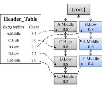
(46) In Figure 3.9, the fuzzy frequent itemsets of {A.Middle, D.Low} with {C.High} can be generated as (A.Middle, C.High, D.Low): 1.8} since the minimum operation is used to find the merged fuzzy value of two nodes. After that, {C.High} can be merged with {A.Middle, D.Low} forming a conditional MFFP tree of {A.Middle, C.High, D.Low}, which is shown in Figure 3.10. Since there is no any nodes existing in the conditional MFFP tree of {A.Middle, C.High, D.Low}, the recursive process for {A.Middle, D.Low} is then terminated.. {A.Middle, D.Low} 1.8. {A.Middle, C.High, D.Low} 1.8. C.High 2.2. NULL. Conditional MFFP-tree with {A.Middle, D.Low}. Conditional MFFP-tree with {A.Middle , C.High, D.Low}. Figure 3.10. The conditional MFFP-tree for {A.Middle, C.High, D.Low}. After {A.Middle} is then recursively processed with {D.Low}, {C.High} is then merged with {D.Low} for recursively processing to generate the conditional MFFP tree of {C.High, D.Low}. Since there is no any nodes in the conditional MFFP tree of {C.High, D.Low}, the recursive process for {C.High, D.Low} is then terminated. After that, the final results of fuzzy frequent itemsets with {D.Low} are shown in. 32.
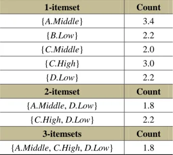
(47) Table 3.7.. Table 3.7. The derived fuzzy frequent itemsets of {D.Low} Fuzzy frequent itemsets. Count. {D.Low}. 2.2. {A.Middle, D.Low}. 1.8. {C.High, D.Low}. 2.2. {A.Middle, C.High, D.Low}. 1.8. The same process is then repeated for the other fuzzy regions until all regions in the Header_Table are processed. After STEP 5, the results of the derived fuzzy frequent itemsets are shown in Table 3.8.. Table 3.8. All derived fuzzy frequent itemsets from the MFFP tree 1-itemset. Count. {A.Middle}. 3.4. {B.Low}. 2.2. {C.Middle}. 2.0. {C.High}. 3.0. {D.Low}. 2.2. 2-itemset. Count. {A.Middle, D.Low}. 1.8. {C.High, D.Low}. 2.2. 3-itemsets. Count. {A.Middle, C.High, D.Low}. 1.8. 33.
(48) CHAPTER 4 Compressed Multiple Fuzzy FP-tree Algorithm In the MFFP tree, the fuzzy regions are sorted in descending order of their locally fuzzy values at each transaction. Two transactions may have the same fuzzy regions but in different ordering, however, would be inserted into the MFFP tree as two different branches. After a large database is processed, the built MFFP tree would have loose and huge structures. In this chapter, the compressed multiple fuzzy FP tree (abbreviated as CMFFP-tree) algorithm is thus proposed to efficiently mine the complete fuzzy frequent itemsets from a set of quantitative transactions. The CMFFP tree inherits the properties of the CFFP tree [25], which sorts fuzzy regions in descending order of their occurrence frequencies to form the updated transactions for constructing the condensed tree structure. Each node has an attached array to store the membership values of itemsets with its super-items in the path via minimum operation.. 4.1 Basic Concepts. 34.
(49) In fuzzy data mining, the intersection operator is used to get the fuzzy count of a fuzzy itemset. According to fuzzy theory, many operations can be adopted for fuzzy interaction; the most commonly used operation is the minimum operation. For example, if a transaction consists of {A.Middle: 0.4, B.High: 0.6}, then the membership value of the fuzzy 2-itemset (A.Middle, B.High) in the transaction is 0.4 0.6, which is 0.4 after the minimum operation. The concept is defined below. Definition 1: A transformed transaction consists of a set of fuzzy items {f1: s1, f2: s2, …, fi: si, …, fn: sn}, where fi is a fuzzy region and si is the transformed fuzzy value of fi , 1 i n . Definition 2: A fuzzy k-itemset in a transformed transaction consists of k fuzzy regions in the transaction and its fuzzy value is the minimum of the fuzzy values of the fuzzy regions. Based on the above definitions, assume that there are two transactions, {f1: s1, f2: s2} and {f1: s3, f2: s4}. The actual fuzzy count of the derived fuzzy 2-itemset (f1, f2) is {min(s1, s2) + min(s3, s4)}, which can easily be proven to be equal to or smaller than min(s1 + s3, s2 + s4). That is, min(s1, s2) + min(s3, s4) min(s1 + s3, s2 + s4). We may then derive the following lemma by induction. Lemma 1: Suppose that there are n transactions {f1: s1, f2: s2}, {f1: s3, f2: s4}, …., {f1: s2n-1, f2: s2n}. The following results may be obtained: min(s1, s2) + min(s3, s4) + …. 35.
(50) + min(s2n-1, s2n) min(s1 + s3 + s5 +…+ s2n-1, s2 + s4 + s6 + … + s2n).. From Lemma 1, it can be easily seen that the minimum of the counts of the two individual fuzzy regions is an upper bound of the actual count of the fuzzy 2-itemset. The concept can also be extended to k-itemsets. This property is used in the proposed three multiple tree structures. However, when transactions are inserted into the tree structures, the way that sort the fuzzy frequent regions in each transaction by their membership values in a descending order, the upper-bound fuzzy counts have the downward-closure property along with the item number. Suppose that there are three transactions, {A.Middle:0.2}, {A.Middle: 0.4, B.High: 0.6}, and {A.Middle: 0.8, B.High: 0.2}. The occurrence frequencies of A.Middle and B.High in the database are respectively calculated as 3 and 2. The actual membership value of the fuzzy 2-itemset {A.Middle, B.High} is 0.6, which is min(0.4, 0.6)+min(0.8, 0.2). However, if the occurrence frequencies are sorted based on the properties of the FP-tree algorithm [13], the three transactions would form a branch as {A.Middle:1.4, B.High:0.8}. The membership value of the fuzzy 2-itemset (A.Middle, B.High) would be calculated as 0.8, which is min(1.4, 0.8). This value is larger than the actual membership value of the fuzzy 2-itemset (A.Middle, B.High). That is, the actual membership value can be calculated using the proposed three multiple tree structures with the downward closure property.. 36.
(51) 4.2 Notation D. the original quantitative database;. n. the number of transactions in D;. T. the i-th transaction in D, 1 i n ;. m Ij. the number of items in D; the j-th item, 1 j m ;. hj. the number of fuzzy regions for Ij. Rjl. the l-th fuzzy region of Ij, 1 l h j ;. vij. the quantitative value of Ij in T;. fijl. the membership value of vij in region Rjl;. countjl. the count of the fuzzy region Rjl in D;. s. the predefined minimum support threshold;. o(Rjl). the occurrence frequency of the fuzzy region Rjl;. C. the set of derived candidate fuzzy itemsets from the CMFFP tree;. 4.3 The CMFFP-tree Construction Algorithm INPUT: A quantitative database consisting of n transactions, a set of membership functions, and a predefined minimum support threshold s. OUTPUT: A compressed multiple fuzzy FP tree (CMFFP tree). STEP 1: Transform quantitative value vij of each item Ij in the i-th transaction into a fuzzy set fij represented as (fij1/Rj1 + fij2/Rj2 + …+ fijh/Rjh) using the given membership functions, where h is the number of fuzzy regions for Ij, Rjl is the l-th fuzzy region of Ij, 1 l h , and fijl is vij’s fuzzy membership value in region Rjl. Note that fijl/Rjl means that the membership value of region Rjl. 37.
(52) is fijl. STEP 2: Calculate the scalar cardinality countjl of each fuzzy region Rjl in the transactions as: n. count jl f ijl . i 1. STEP 3: Check whether the value countjl of the fuzzy region Rjl is larger than or equal to the predefined minimum count n*s. If the count of a fuzzy region Rjl is equal to or greater than minimum count, it can be treated as a fuzzy frequent itemset and put it in the set of L1. That is: L1 = {Rjl | countjl n*s, 1 j m}. STEP 4: Calculate the occurrence frequency o(Rjl) of each fuzzy region in L1. STEP 5: Build the Header_Table by sorting the fuzzy regions (fuzzy frequent itemsets) in L1 in descending order of their occurrence frequencies. STEP 6: Remove the fuzzy regions of the items not existing in L1 from the transactions of the transformed database. Sort the remaining fuzzy regions in descending order of their occurrence frequencies in each transaction. STEP 7: Initially set the root node of the CMFFP tree as {root}. STEP 8: Insert the transactions of the transformed database into the CMFFP tree tuple by tuple. The following two cases may exist. Substep 8-1: If a fuzzy region Rjl in a transaction is at the corresponding 38.
(53) branch of the CMFFP tree, add the membership value fijl of Rjl in the processed transaction to the node of Rjl in the branch.. Calculate. the. membership. values. of. its. super-itemsets with Rjl in the path using the intersection operation. Add the values to the corresponding elements of the array in the node. Substep 8-2: Otherwise, add a node of Rjl at the end of the corresponding branch, set the count of the node as the membership value fijl of Rjl, and calculate the membership values of its super-itemsets with Rjl in the path using the intersection operation. Add values to the corresponding elements of the array in the node. Connect the node of Rjl in the last branch with the current node as a sequence. If there is no such branch with the node of Rjl, insert a node-link from the entry of Rjl in the Header_Table to the added node.. In STEP 8, a corresponding branch is the branch built in the CMFFP tree according to the sorted fuzzy regions in the transformed transaction. Note that the transformed fuzzy frequent regions from a given item cannot form the fuzzy frequent. 39.
(54) itemsets because they would be meaningless; they are thus not stored in the attached array of a tree node.. 4.4 An. Example. of. the. CMFFP-tree. Construction Algorithm. In this section, an example is given to illustrate how to construct a CMFFP tree from quantitative transaction data. The quantitative database is shown in Table 4.1, which database consists of 6 transactions and 5 items, denoted A to E.. Table 4.1. Six transactions with purchased items and its quantitative values TID. Items. 1. (A:5) (C:10) (E:9). 2. (A:8) (B:2) (C:3). 3. (B:3) (C:9). 4. (A:7) (C:9) (D:3). 5. (A:5) (B:2) (C:5). 6. (A:3) (C:10) (D:4) (E:2). Assume that the fuzzy membership functions are the same for all items shown in Figure 4.1. In this example, amounts are represented by three fuzzy regions: {Low}, {Middle}, and {High}. Thus, three fuzzy membership values are produced for each item in a transaction according to the predefined membership functions in Figure 4.1. 40.
(55) Note that the proposed approach also works when the membership functions of the amounts for the items are not the same.. Low. Middle. High. Membership value. 1. 0. 1. 6. 11. Amount. Figure 4.1. Membership functions used in this example. The CMFFP tree for this example is thus constructed using the proposed approach as follows. STEP 1: The quantitative values of the items in the transactions are represented as fuzzy sets using the membership functions shown in Figure 4.1. Take item {A} in transaction 1 as an example to illustrate the procedure. The amount “5” of A can be converted into the fuzzy set (. 0.2 0.8 ) by the membership functions in , A.Low A.Middle. Figure 4.1. This step is repeated for the other items in Table 4.1, and the results are shown in Table 4.2.. 41.
(56) Table 4.2. Fuzzy sets transformed from Table 4.1 TID. Items. 1. (. 0.2 0.8 0.2 0.8 0.4 0.6 , ), ( , ), ( , ) A.Low A.Middle C.Middle C.High E.Middle E.High. 2. (. 0.6 0.4 0.8 0.2 0.6 0.4 , ), ( , ), ( , ) A.Middle A.High B.Low B.Middle C.Low C.Middle (. 3 (. 4. 6. 0.8 0.2 0.4 0.6 0.6 0.4 , ), ( , ), ( , ) A.Middle A.High C.Middle C.High D.Low D.Middle (. 5 (. 0.6 0.4 0.4 0.6 , ), ( , ) B.Low B.Middle C.Middle C.High. 0.2 0.8 0.8 0.2 0.2 0.8 , ), ( , ), ( , ) A.Low A.Middle B.Low B.Middle C.Low C.Middle. 0.6 0.4 0.2 0.8 0.4 0.6 0.8 0.2 , ), ( , ), ( , ), ( , ) A.Low A.Middle C.Middle C.High D.Low D.Middle E.Low E.Middle. STEP 2: The scalar cardinality of each fuzzy region in transactions is calculated as the count value. Take the fuzzy region {A.Low} as an example to explain the procedure. {A.Low} appears in transactions 1, 5, and 6, and its scalar cardinality is calculated as (0.2 + 0.2 + 0.6) (= 1.0). The step is repeated for the other regions; the results are shown in Table 4.3.. Table 4.3. Counts of fuzzy regions Item. Count. Item. Count. Item. Count. A.Low. 1.0. C.Low. 0.8. E.Low. 0.8. A.Middle. 3.4. C.Middle. 2.4. E.Middle. 0.6. A.High. 0.6. C.High. 2.8. E.High. 0.6. B.Low. 2.2. D.Low. 1.0. B.Middle. 0.8. D.Middle. 1.0. B.High. 0.0. D.High. 0.0. 42.
(57) STEP 3: The fuzzy regions in Table 4.3 are then checked against the predefined minimum count, which is calculated as (6 * 0.2) (= 1.2). For example, the counts for {A.Low}, {A.Middle}, and {A.High} are 1.0, 3.4, and 0.6, respectively. Since the count for {A.Middle} is larger than the minimum count, {A.Middle} is then kept for the subsequent mining process. The satisfied fuzzy regions are considered as fuzzy frequent itemsets and kept them in the set of L1 for later building the CMFFP tree. Thus, L1 = {A.Middle: 3.4, B.Low: 2.2, C.Middle: 2.4, C.High: 2.8}. STEPs 4 & 5: The occurrence frequency of each fuzzy region in L1 is also calculated while executing the above step. For example, fuzzy region {A.Middle} appears in transactions 1, 2, 4, 5, and 6. Thus, its occurrence frequency is set as 5. The other fuzzy regions are processed in the same way, and the results are shown in Table 5.4.. Table 4.4. The fuzzy regions, its counts and its occurrence frequencies Item. Count. Occurrence frequency. A.Middle. 3.4. 5. B.Low. 2.2. 3. C.Middle. 2.4. 6. C.High. 2.8. 4. The fuzzy frequencies regions in L1 are then sorted in descending order according. 43.
(58) to their occurrence frequencies to form the Header_Table of the CMFFP tree. The results are shown in Figure 5.2.. Header_Table Fuzzy regions. Count. C.Middle. 2.4. A.Middle. 3.4. C.High. 2.8. B.Low. 2.2. Figure 4.2. The built Header_Table. STEP 6: The fuzzy regions not existing in L1 are then removed from each transaction in Table 4.2. The remaining fuzzy regions at each transaction are then sorted according to their occurrence frequencies. The updated transactions of the sorted results are shown in Table 4.5.. Table 4.5. The updated transactions for constructing the CMFFP tree TID. Fuzzy regions. 1. 0.2 0.8 0.8 , , C.Middle A.Middle C.High. 2. 0.4 0.6 0.8 , , C.Middle A.Middle B.Low. 3. 0.4 0.6 0.6 , , C.Middle C.High B.Low. 4. 0.4 0.8 0.6 , , C.Middle A.Middle C.High. 44.
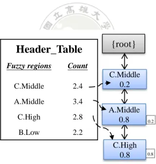
(59) 5. 0.8 0.8 0.8 , , C.Middle A.Middle B.Low. 6. 0.2 0.4 0.8 , , C.Middle A.Middle C.High. STEP 7: The root of the CMFFP tree is initially set as {root}. STEP 8: The updated transactions in Table 4.5 are used to construct the CMFFP tree tuple by tuple, from the first transaction to the last one. Each node consists of not only the fuzzy frequent 1-itemset with its membership value, but also an attached array that stores the membership values with its super-itemsets in the path obtained using the intersection operation, which is minimum operation here. Take the first transaction, (. 0.2 0.8 0.8 ), as an example to illustrate the process. A , , C.Middle A.Middle C.High. new node {C.Middle} with a membership value of 0.2 is created and linked to the root. Since {C.Middle} is the first item in the path, it is unnecessary to find the membership values of its super-itemsets from the transaction. Next, the node {A.Middle} with a membership value of 0.8 is created and linked to the node {C.Middle}. In this example, there is only a super-itemset {A.Middle} in the path, thus the membership value is then calculated as {C.Middle A.Middle}, which is (0.2 0.8) (= 0.2). The super-itemset {C.Middle, A.Middle} and its membership value 0.2 are then stored in the array of the {A.Middle} node. Next, the node {C.High} with a membership value of 0.8 is created and linked to the node {A.Middle}. In this. 45.
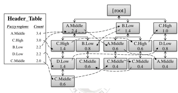
(60) example, there are two super-itemsets {A.Middle} and {C.High} in the path. Since {C.Middle} and {C.High} are both associated with item C, it is meaningless to combine these two fuzzy regions. The membership value of {A.Middle, C.High} is then calculated as (A.Middle C.High), which is (0.8 0.8) (= 0.8), and stored in the array of the {C.High} node. Three node-links from nodes {C.Middle}, {A.Middle}, and {C.High} in the Header_Table are respectively connected to its generated nodes of the CMFFP tree. The results obtained after the first transaction is processed are shown in Figure 4.3.. Header_Table Fuzzy regions. {root}. Count. C.Middle. 2.4. A.Middle. 3.4. C.High. 2.8. B.Low. 2.2. C.Middle 0.2 A.Middle 0.8 C.High 0.8. 0.2. 0.8. Figure 4.3. The CMFFP tree after the first transaction has been processed. The same process is then executed for the other transactions. The final Header_Table and the constructed CMFFP tree are shown in Figure 4.4.. 46.
(61) root. Header_Table Fuzzy regions. Count. C.Middle. 2.4. A.Middle. 3.4. C.High. 2.8. B.Low. C.Middle 2.4. A.Middle 3.4. C.High 0.6. 2.0. 2.2 C.High 2.2. 1.8. B.Low 1.6. 1.2 1.4 1.2. B.Low 0.6. 0.4 0.6. Figure 4.4. The finally constructed CMFFP tree. The constructed CMFFP tree can be used for deriving all the fuzzy frequent itemsets without the need to generate conditional patterns. The proposed CMFFP-mine algorithm, which used the CMFFP tree, is described in the next section.. 4.5 The CMFFP-mine Mining Algorithm After the CMFFP tree is constructed, the fuzzy frequent itemsets with more than one fuzzy region can be found using the proposed CMFFP-mine algorithm. The details of the proposed algorithm are given below.. INPUT: The built CMFFP tree, its corresponding Header_Table, and the pre-calculated minimum count n*s. OUTPUT: The fuzzy frequent itemsets. STEP 1: Process the fuzzy regions in the Header_Table one by one from bottom to 47.
(62) top using the following steps. Let the currently processed fuzzy region is set as Rjl. STEP 2: Find all nodes with fuzzy region Rjl in the CMFFP tree through the sequenced connection between nodes. STEP 3: The fuzzy itemsets with fuzzy region Rjl and their membership values are extracted from the array in each extracted node found in STEP 2. STEP 4: Sum the membership values of the same fuzzy itemsets. STEP 5: Repeat STEPs 2 to 4 for the other fuzzy regions until all fuzzy regions in the Header_Table are processed. The results are then put in the set of C. STEP 6: Check whether the membership value of each fuzzy itemset in C is greater than or equal to the predefined minimum count. Output the satisfied fuzzy itemsets as the fuzzy frequent itemsets with the currently processed fuzzy region Rjl.. After STEP 6, the desired fuzzy frequent itemsets can be found from the built CMFFP tree. An example is given below to illustrate the algorithm.. 4.6 An Example of the CMFFP-mine Algorithm For the built CMFFP tree in Figure 4.4, the proposed CMFFP-mine algorithm is. 48.
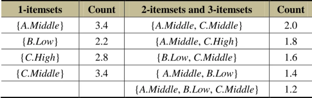
數據
+7

相關文件
In this chapter we develop the Lanczos method, a technique that is applicable to large sparse, symmetric eigenproblems.. The method involves tridiagonalizing the given
For the proposed algorithm, we establish a global convergence estimate in terms of the objective value, and moreover present a dual application to the standard SCLP, which leads to
Like the proximal point algorithm using D-function [5, 8], we under some mild assumptions es- tablish the global convergence of the algorithm expressed in terms of function values,
Microphone and 600 ohm line conduits shall be mechanically and electrically connected to receptacle boxes and electrically grounded to the audio system ground point.. Lines in
Given a graph and a set of p sources, the problem of finding the minimum routing cost spanning tree (MRCT) is NP-hard for any constant p > 1 [9].. When p = 1, i.e., there is only
• When this happens, the option price corresponding to the maximum or minimum variance will be used during backward induction... Numerical
• When this happens, the option price corresponding to the maximum or minimum variance will be used during backward induction... Numerical
First, when the premise variables in the fuzzy plant model are available, an H ∞ fuzzy dynamic output feedback controller, which uses the same premise variables as the T-S
