波束可掃描之波導漏波天線設計－理論分析與天線製作量測

(1)

國

立

交

通

大

學

電信工程學系

博士論文

波束可掃描之波導漏波天線設計－理論分析與

天線製作量測

A Beam Adjustable Leaky-Wave Antenna Using a Moveable

Dielectric Slab inside a Waveguide－Theoretical Analysis and

Experimental Studies

研究生：蕭承麒

指導教授：黃瑞彬博士

(2)

波束可掃描之波導漏波天線設計－理論分析與天線製作量測

A Beam Adjustable Leaky-Wave Antenna Using a Moveable

Dielectric Slab inside a Waveguide－Theoretical Analysis and

Experimental Studies

研究生：蕭承麒 Student：Cherng Chyi Hsiao

指導教授：黃瑞彬博士 Advisor：Dr. Ruey Bing Hwang

國立交通大學

電信工程學系

博士論文

A Dissertation

Submitted to Department of Communication Engineering College of Electrical Engineering and Computer Science

National Chiao Tung University in Partial Fulfillment of the Requirements

for the Degree of Doctor of Philosophy

in

Communication Engineering

July 2005

Hsinchu, Taiwan, Republic of China

(3)

波束可掃描之波導漏波天線設計－理論分析

與天線製作量測

國立交通大學電信工程學系研究生：蕭承麒指導教授：黃瑞彬博士摘要本論文旨在以理論分析、軟體模擬、天線製作及實驗量測，來探討波束可掃描之波導漏波天線的可行性。為使天線具有波束掃瞄的能力，於槽孔導波管內的縱向軸上，置放一介電板，因槽孔導波管的橫向電場屬不均勻分布，變化該介電板置放在槽孔導波管內橫軸向的位置，對槽孔導波管內的電磁場產生不等量的干擾，因此改變漏波之縱向傳波常數，以改變漏波波束之主輻射角，令天線具有波束掃瞄之能力。在理論分析部分，使用“縱向諧振方程＂，推導色散關係式，以計算波導傳波常數的相位常數及耗損常數。本論文中之理論分析、軟體模擬及實驗量測所得之天線場型分布及波束之主輻射角等數據，都很接近，證明本波束可掃瞄天線之設計，確為可行。在 Ku 波段操作，天線波束掃描之範圍，可達23度。

(4)

A Beam Adjustable Leaky-Wave Antenna Using a Moveable

Dielectric Slab inside a Waveguide－Theoretical Analysis and

Experimental Studies

Student: Cherng-Chyi Hsiao Advisor: Dr. Ruey-Bing Hwang

Department of Communication Engineering

National Chiao Tung University

Abstract

In this dissertation, we presented a beam adjustable antenna made up of a slitted waveguide

and a dielectric slab. In order to steer the radiation main-beam angle, we changed the phase

constant of the waveguide mode by inserting a moveable dielectric slab to perturb its field

distribution. The direction of radiation main-beam can be steered dynamically by changing

the position of the dielectric slab. In theoretical analysis, the dispersion relation to obtain the

phase and attenuation constants, were determined by solving the transverse resonance

equation. An agreement between the theoretical and experimental radiation pattern verifies

the beam-steering mechanism. Up to 23o beam-steering angle can be achieved in Ku-band

(5)

誌

謝

非常感謝我的指導教授黃瑞彬博士，經過他的嚴密指導，終於使本論文得以呈現。同時也要感謝彭松村教授和尉應時教授的指導。感謝王惠民和江丕揚先生的通力合作。感謝 309 電磁應用實驗室的每一位夥伴的協助。感謝我的家人，極有耐心陪我度過這段日子。感謝每一位曾經幫助我的人。

(6)

TABLE OF CONTENTS ABSTRACT (Chinese) ……… i ABSTRACT (English) ……… ii ACKNOWLEDGEMENTS ……… iii TABLE OF CONTENTS ……… iv LIST OF TABLES ……… vi

LIST OF FIGURES ……… vii

CHAPTER 1 INTRODUCTION……… 1

1.1 Motivation of This Research……… 1

1.2 Background of This Research and the Related Literature 1 CHAPTER 2 STATEMENT OF PROBLEM AND METHODS OF ANALYSIS……… 4 2.1 Basic Theory of the leaky-Wave Antenna ……… 4

2.2 Perturbation Method……… 5

2.3 Mathematical Analysis of the Leaky Wave Antenna…… 8

2.3.1 Basic Idea of the Beam Steering Scheme……… 8

2.3.2 Basic Idea and Analysis Model……… 9

2.3.3 Eigen-Modes in Closed Waveguide……… 9

2.3.4 Transmission Line Network Representation……… 11

2.3.5 Transverse Resonance Equation……… ₁₂

2.3.6 Far Field Radiation Pattern……… ₁₃

(7)

CHAPTER 3

Fabrication, Measurement Setup, and Comparison between Experimental and Theoretical Results…………

24 3.1 Fabrication of this Antenna and the Measurement

Setup ……… 24

3.2

Measurement Setup……… ₂₄

3.3 Comparison Between Experimental and Theoretical

Results……… 25

CHAPTER 4 _{Applications ………}

67

4.1 Possible Application of the Fabricated Antenna ……… 67

CHAPTER 5 Concluding Remarks……… 72

APPENDIX I ……… 73 REFERENCES ……… 77 PERSONAL INFORMATION (CHINESE) ……… 81 PUBLICATION LIST ……… 82

(8)

List of Figures

1. Figure1. The leaky wave above a partially open waveguide…………... (16)

2. Figure2. A beam steering antenna for the B-29 airborne radar implemented in WWII by perturbation of the waveguide sidewall…………...………... (17)

3. Figure3(a). Structural parameters and the coordinate systems of the leaky waveguide antenna………..………... (18)

4. Figure3(b). A slitted waveguide with bottom plate removed……. …... (19)

5. Figure3(c). A slitted waveguide with bottom plate removed and with input and output flanges……….……. ……... (19)

6. Figure3(d). A slitted waveguide with bottom plate removed and with coaxial to waveguide terminations at input port and output port………. ……... (20)

7. Figure3(e). A slitted waveguide together with a metal block which has a additional dielectric slab on top of it………....………. ……...(20)

8. Figure3(f). A well refurbished beam steering antenna………..(21) 9. Figure3(g). Front view of the leaky wave antenna………(22)

10. Figure3(h). Equivalent transmission line network of the leaky wave antenna……….(22)

11. Figure 4(a). Original electromagnetic fields with sources enclosed by a closed surface S………(23)

12. Figure4(b). Equivalent sources on S to produce equivalent electromagnetic fiels………... (23)

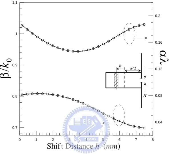
13. Figure5. Normalized phase constants and attenuation constants as a function of shift distance for case 1 dielectric slab inside the leaky waveguide…... (31)

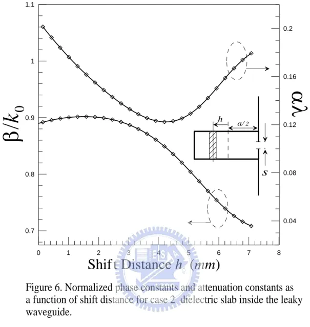
14. Figure6. Normalized phase constants and attenuation constants as a function of shift distance for case 2 dielectric slab inside the leaky waveguide……… (32)

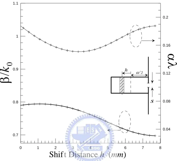
15. Figure7. Normalized phase constants and attenuation constants as a function of shift distance for case 3 dielectric slab inside the leaky waveguide……… (33)

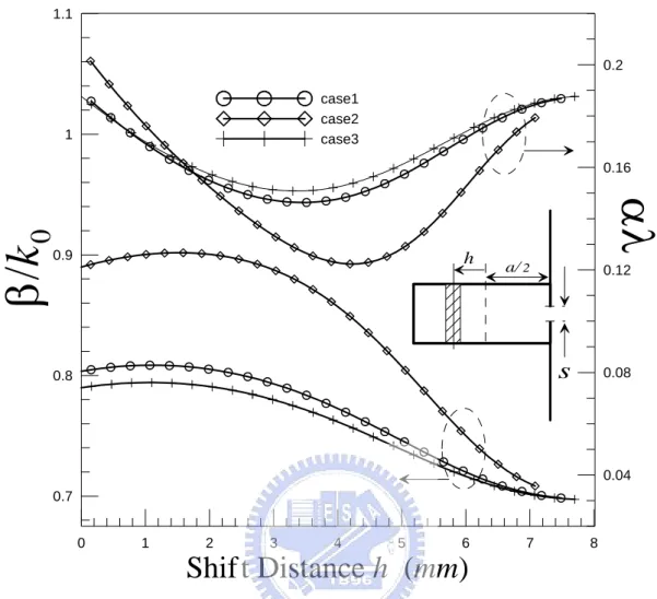
16. Figure8. Normalized phase constants and attenuation constants as a function of shift distance for case 1, case 2 and case 3 dielectric slab inside the leaky waveguide……… (34)

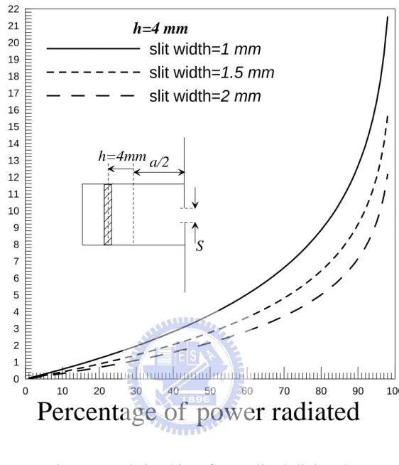
17. Figure9. Relationships of normalized slit lengths a function of percentage of radiation power, the slit widths are 1, 1.5, and 2mm. The dielectric slab is case 2 and being placed at t h=4 mm………... .(35)

18. Figure10. Theoretical(MTLM) and experimental radiation patterns of case 1 dielectric slab with relative dielectric constant and thickness are 2.55 and 0.81mm respectively, while shift distance h=0mm………..(36)

(9)

slab with relative dielectric constant and thickness are 2.55 and 0.81mm respectively, while shift distance h=1mm………. (37)

20. Figure12. Theoretical(MTLM) and experimental radiation patterns of case 1 dielectric slab with relative dielectric constant and thickness are 2.55 and 0.81mm respectively, when shift distance h=2mm………. (38)

21. Figure13. Theoretical(MTLM) and experimental radiation patterns of case 1 dielectric slab with relative dielectric constant and thickness are 2.55 and 0.81mm respectively, while shift distance h=3mm………. (39)

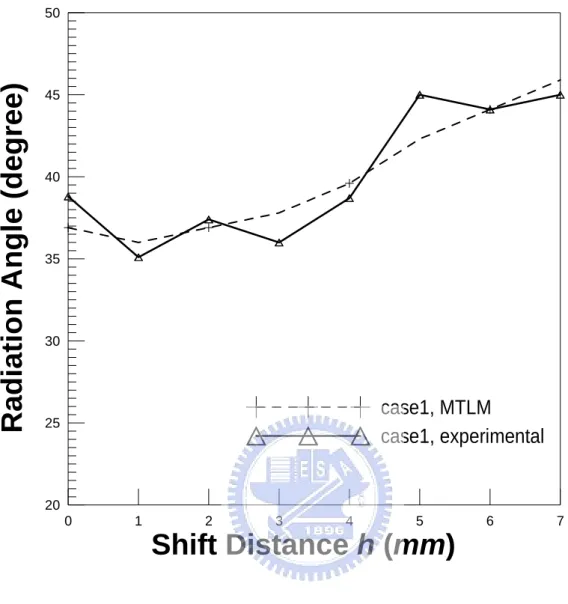
26. Figure18. Radiation angles of the leaky-wave antenna as the functions of the shift distances using case 1 dielectric slab. Antenna radiation angles are obtained by modal transmission line method and experimental tests………. (44)

27. Figure19. Theoretical(MTLM) and experimental antenna radiation patterns using case 2 dielectric slab with relative dielectric constant and thickness 2.55 and 1.62mm respectively, while shift distance h=0mm, while shift distance h=0mm………. (45)

28. Figure20. Theoretical(MTLM) and experimental antenna radiation patterns using case 2 dielectric slab with relative dielectric constant and thickness 2.55 and 1.62mm respectively, while shift distance h=1mm……… (46)

29. Figure21. Theoretical(MTLM) and experimental antenna radiation patterns using case 2 dielectric slab with relative dielectric constant and thickness 2.55 and 1.62mm respectively , while shift distance h=2mm………(47)

30. Figure22. Theoretical(MTLM) and experimental antenna radiation patterns using case 2 dielectric slab with relative dielectric constant and thickness 2.55 and 1.62mm respectively, while shift distance h=3mm……….(48)

31. Figure23. Theoretical(MTLM) and experimental antenna radiation patterns using case 2 dielectric slab with relative dielectric constant and thickness 2.55 and 1.62mm respectively, while shift distance h=4mm……….(49)

(10)

32. Figure24. Theoretical(MTLM) and experimental antenna radiation patterns using case 2 dielectric slab with relative dielectric constant and thickness 2.55 and 1.62mm respectively, while shift distance h=5mm………..(50)

35. Figure27. Radiation angles of the leaky-wave antenna as the functions of the shift distances using the case 2 dielectric slab. Antenna radiation angles are obtained by theoretical modal transmission line method and experimental tests……… (53)

36. Figure28. Antenna radiation patterns obtained by using the modal transmission line method (MTLM) and the experiment. Case 2 dielectric slab was used, the relative dielectric constant and thickness (mm) of the dielectric slab are 2.55 and 1.62 respectively, and the shift distances h are 0, 4 and 7mm………..(54)

37. Figure29. Theoretical (MTLM) and experimental radiation patterns using case 3 dielectric slab with relative dielectric constant and thickness 3.84 and 0.38mm respectively, while shift distance h=0mm……….(55)

38. Figure30. Theoretical (MTLM) and experimental radiation patterns using case 3 dielectric slab with relative dielectric constant and thickness 3.84 and 0.38mm respectively, while shift distance h=1mm………. (56)

40. Figure32. Theoretical (MTLM) and experimental radiation patterns using case 3 dielectric slab with relative dielectric constant and thickness 3.84 and 0.38mm respectively, while shift distance h=3mm…... (58)

(11)

dielectric slab with relative dielectric constant and thickness 3.84 and 0.38mm respectively, while shift distance h=7mm………. (62)

45. Figure37. Radiation angles of the leaky-wave antenna as the functions of the shift distances using the case 3 dielectric slab. Antenna radiation angles are obtained by theoretical modal transmission line method and experimental tests……… (63)

46. Figure38. Radiation angles of the leaky-wave antenna as the functions of the shift distances using the case 1, case 2 and case 3 dielectric slab. Antenna radiation angles are obtained by theoretical modal transmission line method and experimental tests………....(64)

47. Figure39. Antenna radiation pattern obtained by modal transmission line method, experimental test and Finite Integration Technique (FIT of CST Microwave Studio), using case 2 dielectric slab, and the shift distance of the dielectric slab are 0 and 7mm, respectively………...(65)

48. Figure40. Antenna efficiency and gain of the leaky-wave antenna as a function of the shift distance h (mm) using the case 2 dielectric slab, which has dielectric constant 2.55 and thickness 1.62 mm, respectively……… (66)

49. Figure41. Radiation angles of a leaky-wave antenna versus the shift distance of the dielectric slab h, obtained by using the theoretical modal transmission line method, the operating frequency is 77 GHz, the relative dielectric constant of the dielectric slab is

2.55, and the thicknesses are 0.22 and 0.3 mm

respectively……… (69)

50. Figure42. Antenna radiation patterns obtained from modal transmission line method, operating at 77 GHz, which has 6.25λ (24.35 mm) as slit length, the relative dielectric constant and thickness (mm) of the dielectric slab are 2.55 and 0.3 respectively, the shift distances are 0, 0.3, 0.6, 0.9, and 1.125mm. The corresponding maximum radiation angles are at 34.2, 34.2, 39.6, 49.5 and 54.9 degrees, respectively……….. (70)

51. Figure43. Theoretical radiation patterns of a leak-wave antenna, operating at 77GHz, the slit length was 125mm, the relative dielectric constant and thickness (mm) of the dielectric slab are 2.55 and 0.3 respectively, the shift distances are 0, 0.3, 0.6, 0.9, and

1.125mm. The corresponding maximum radiation angles are at 34.2, 34.4, 39.9, 49.3,

(12)

CHAPTER 1. INTRODUCTION

1.1 Motivation of This Research

R

ecently, the demands of integrated data packets over RF carriers are increasing rapidly. As the number of users in a given wireless-communication systems increases, the service quality of the system becomes more and more stringent. To warranty a reliable communication over a radio channel, the system should overcome interferences like multi-path fading. By using the beam-steering technology as the smart antenna achieves in wireless communication, it is possible to enlarge system coverage, to achieve interference mitigation, and to improve signal to noise ratio. The beam steering techniques thus have recently received increasing interest to improve the performance of a wireless radio system. It has been shown how smart antennas, with spatial processing, can provide substantially additional improvement when used with CDMA digital-communication systems [1]. Perhaps the most important feature of a beam steering antenna system is its capability to remove co-channel interference. Co-channel interference is the radiation from cells that use the same set of channel frequencies in the system. Thus, co-channel interferences in the transmitting mode can be reduced by focusing a directive beam in the direction of a desired user and nullifying in the directions of the other users. In receiving mode, co-channel interference can be reduced by pointing antenna to the directional location of the signal source. There are also many applications in military or space area that require fast beam steering capability for the tracking in the direction of an incoming signal.

It is based on these reasons to develop a simple, low-cost, reliable, and easy to operate beam steering antenna without using the conventional expensive ferrite or solid-state phase shifters for the applicable needs of wireless application.

1.2 Background of This Research and the Related Literature

E

ver since the first invention of the first directional antenna, a lot of techniques have been developed to steer the antenna main beam. Gimbaled type antenna system was developed in the beginning to direct the antenna main beam with fixed pattern to a desired direction. The

(13)

advance of the antenna in a radar system was detailedly recorded in [2]. Those mechanical scanning radar systems are inherently characterized by consuming considerable dynamic response time, and may not be acceptable for some systems, which require specifically fast reaction time.

Electronic beam steering has been developed for a long time by using a phased array antenna through shifting the phase in each array element [3-8]. The electronic beam-steering system possesses a fast switching rate; however, the mechanical type has a consistent radiation beam pattern during the beam scanning [9-10]. Electronic beam steering needs, generally, expensive ferrite or solid-state phase shifters or a complex beam-forming network. Therefore, such a system is not cost-effective and is mainly applied in military or space-borne systems. Nowadays, because of the demands for beam-steering antenna system in wireless communication system and ITS (Intelligent Transportation System) applications, a low-cost and robust beam-steering system attracts considerable attentions.

Various novel beam-steering techniques have been proposed in the past. To mention a few, an actuator perturbing the propagation constant of a microstrip line was used as a phase shifter [11-13]. A moveable grating was used to perform a beam-steering leaky wave antenna [14]. They also used the moveable metal plate to perturb the dielectric image line and then to change the phase constant of the transmission line [15-17]. The grating with PIN diodes or MEMS-based switch was utilized to switch the direction of radiation main beam between two angles [18-20]. A re-configurable photonic band-gap structure was employed to serve as a phase shifter in a phased array system [21]. A slotted-microstrip line perturbed by metal strips was developed to act as a multi-functional device including the phase shifter and feeding network [22]. Some researchers used the photo-induced semiconductor plasma layer as a re-configurable grating antenna to dynamically change the phase constant and then scan the beam pattern [23].

Waveguide-based leaky-wave antennas have been developed for many years. For example, the slits on the metal waveguide sidewall were implemented theoretically and experimentally [24-31]. The slitted leaky waveguide array for mobile reception of DBS (direct broadcast from satellite) were successfully designed and implemented by Ando [32-35]. This paper theoretically and experimentally demonstrates the feasibility of a novel low-cost beam-steering antenna based on a leaky-wave structure. The structure under consideration is a rectangular waveguide cut with a slit in the center of the waveguide narrow wall. The theoretical formulation was well developed by using model transmission line method [28-30].

(14)

To add the beam-steering capability to the leaky-wave antenna, we added a dielectric slab longitudinally inside the slitted waveguide. Moving the dielectric slab along the transverse direction, the electric and magnetic fields in the waveguide are perturbed. Consequently, the propagation constant, including the phase and attenuation constants of the leaky mode, varies accordingly. Furthermore, the leaky-wave beam patterns could be changed.

In the theoretical analysis, we model the structure as a slitted waveguide filled with inhomogeneous medium. The transverse resonance equation was employed to calculate the dispersion relation of the waveguide. The finite integration method (FIT), CST Microwave Studio, was also used to compute the radiation pattern. Besides, we fabricated an antenna and measured its far-field radiation pattern under various perturbation conditions (displacement of the dielectric slab away from the waveguide center). Three samples of dielectric slabs were used to examine the beam-steering characteristics. Good agreement between theoretical and experimental results verifies the present beam steering mechanism.

(15)

CHAPTER 2. STATEMENT OF PROBLEM AND METHODS OF ANALYSIS

2.1 Basic Theory of the Leaky-Wave Antenna

R

adiation from a continuous uniform slitted waveguide has been known as a traveling wave with a complex propagation constant

(

k_z =β_z− jα_z

)

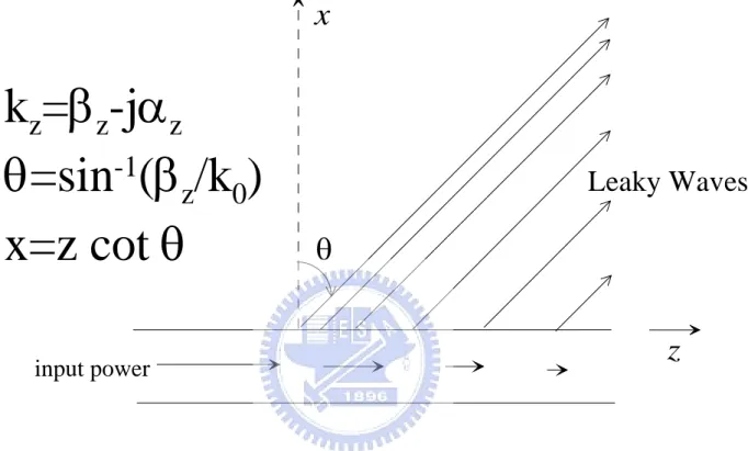
. This traveling wave propagates along the waveguide with its phase velocity greater than that of light, and its amplitude being continuously attenuated as it travels. Thus, the waves feature having continuous leakage of energy and is known as leaky waves. In figure1, a leaky wave above a partially open waveguide together with its coordinate system is given here to demonstrate the leaky wave phenomenon [36-37]. Let the wave-number in the x, y, and z directions be , and ,

respectively. And assuming the system is y-axis independent, that is is zero, such that

x k k_y k_z y k z z z j k =β − α (1a) x x x j k =β − α (1b)

Let the free space wave number bek0, then

(

) (

)

(

x x z z

)

(

x x z z

)

z z x x z x j j j k k k α β α β α β α β α β α β + − − + − = − + − = + = 2 2 2 2 2 2 2 2 2 2 0 (2)

The imaginary part of the above term must vanish, so

z z x x z z x x α β α β α β α β − = = + 0 (3) z

β , α_z and β_x are all positive and real for a traveling leaky wave, we have negative α_x. In the region x>0, the leaky structure radiates with wave amplitude variation given as,

(4) x j x _x x _e e−α ⋅ −β

This corresponds to an exponentially increasing of wave amplitude in the x direction. Though it may seem unphysical, it does represent the field solution in the restricted region of an open waveguide. Again in figure 1, the semi-infinite uniform leaky waveguide is fed by a closed waveguide. The radiation slot of the leaky structure lies in the x=0 plane. It starts radiation at z=0 and the field may extend in the positive z direction. That is, the leaky wave

(16)

ever increases its amplitude as it propagates in the x direction. Despite the improper transverse characteristics, leaky wave can validly represent the radiation field within a sector of space, that is, the portion of space lined in figure 1. And they can never reach infinity unless the source is placed infinitely far away, which means the feeding waveguide is infinitely far away (this is the case not physically realizable). To show the confined region where the leaky wave validates the representation of the radiation fields, let θ be the angle of radiation departed from broadside, and φ =π −θ

2 be the angle departed from end-fire of

the leaky wave antenna, given as ,

g λ λ θ 1 sin− = (5a) or 0 1 sin k z β θ ₌ − (5b) or 0 1 cos k z β φ ₌ − (5c) where z g _β π

λ = 2 is the guide wavelength of the leaky wave in the z direction, k0 and 　λ are

the free space wave-number and wavelength, respectively. Since the amplitude of the leaky wave decays as the wave propagates along the z direction, the amount of radiation per unit length decreases with increasing z. Note that at any point z>0, the field intensity increases along the x direction up to x= z⋅tanφ. In this region, the field amplitude depends on x as given in equation 4. For x> z⋅tanφ the field intensity must decrease drastically in this region. So, confined in the region x< z⋅tanφ, the leaky wave has finite amplitude and is a valid representation of the radiation field.

2.2 Perturbation Method

I

t is known that the electromagnetic field problems can be expressed in integral integration form or in differential equation form. While the differential equation form gives an exact solution of the electromagnetic problem, on the contrast, the integral equation form is especially useful for obtaining approximate solution. Owing to the above characteristics, the integral equation can be employed in perturbation method for approximate solutions of propagation constant of the specified waveguide systems.

(17)

To “perturb” means to change the status of a system slightly. The perturbation method is useful to calculate the changes of a physical quantity due to a small change in the system. There are two circumstances involved in the analysis of a perturbation system. First is the “unperturbed” one, which is with known solution of certain parameters. Then is the “perturbed” one, which is perturbed slightly from the “unperturbed” one in the system. Considering two types of perturbations in a cylindrical waveguide, or a waveguide has identical cross section. One type is on the perturbation of the width of the waveguide wall, and the other type is on the addition of a dielectric material inside the waveguide. The following perturbation formulae for the change in propagation constant in the loss-free waveguide are derived in the Harrington’s textbook [38], however we re-write, use the results, and modify the results to show the physical insight of the two kinds of perturbations mentioned above for beam steering. In the first case the perturbation is on the constituent material inside the waveguide, the change of phase constant from unperturbed value β₀to β due to perturbation is given as:

(

)

(

)

∫∫

⋅ × + × ⋅ × ∆ + ⋅ ∆ = − S S ds z h e h e ds z h e e e 0 * 0 * 0 0 * 0 * 0 0 µ ε ω β β (6)

And, in the case of a waveguide wall perturbation, the change of phase constant from unperturbed value β₀to β due to perturbation is given as:

(

)

(

)

∫∫

′

∫

∗ ∗ ∆ ⋅ × + × ⋅ × − = − S C ds z h e h e dl n h e j 0 0 0 0 0 β β (7)

In the case of shallow, smooth deformation of the waveguide wall, e and h can be approximated by e0 and h0, respectively. So, equations (6) and (7) can be approximated by

(

)

∫∫

⋅ × + × ⎟ ⎠ ⎞ ⎜ ⎝ ⎛_∆ ₊_∆ ≈ − S S ds z h e h e ds h e 0 * 0 0 0 * 0 2 0 2 0 0 µ ε ω β β (8a) and

(

)

(

)

∫∫

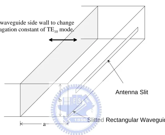
′ ∗ ∗ ∆ ⋅ × + × − ≈ − S S ds z h e h e ds e h 0 0 0 2 0 2 0 0 ε µ ω β β (8b)

An example demonstrates waveguide perturbation is shown in figure 2. It shows a slitted waveguide beam steering antenna. The idea of this beam steering mechanism is to change the longitudinal field propagation constant by changing the waveguide width, that is, by

(18)

deforming the waveguide sidewall longitudinally. Concerning the dominant TE10 mode, the

operating region where the transverse fields are perturbed is with weak electric field strength but strong magnetic field strength. In this case equation (8b) can be reduced to

(

)

∫∫

′

∫∫

∗ ∗ ∆ ⋅ × + × ≈ − S S ds z h e h e ds h 0 0 0 2 0 0 µ ω β β (9)

Change of the propagation constant is approximately proportional to the magnetic field energy stored in the deformed region of the waveguide transverse plane, where magnetic field is of the strongest strength. The slitted waveguide antenna steers its main beam by changing its width of waveguide wall. Assuming that the perturbation is shallow and slight, and the magnetic field strength can similarly as above assumed to be approximately constant over the region of waveguide deformation. Then equation (9) can be further reduced to

₍

₎

b ds z h e h e a h S t ⋅∆ ⎟ ⎟ ⎠ ⎞ ⎜ ⎜ ⎝ ⎛ ⋅ × + × ≈ −

∫∫

′ ∗ ∗ 0 0 0 2 0 µ ω β β (10)

Where a is the height of the waveguide, ∆ represents the deformed width of the waveguide, b

and ht is the magnetic field strength in the deformed waveguide region. Note that the change

in propagation constant depends nearly linearly on the deformation width in the waveguide. This technique has been realized and demonstrated successfully during WWII on the air-borne beam steering radar developed for the aircraft B-29 bomber [2].

The other case of inserting a thin dielectric slab in the waveguide with moderately low relative dielectric constant as shown in figure 3(a), that is we have slight dielectric perturbation. Then equation (8a) becomes

(

)

∫∫

×

∫∫

+ × ⋅ ∆ ≈ − S S ds z h e h e ds e 0 * 0 0 0 * 0 2 0 0 ε ω β β (11)

It is obvious that maximum change in propagation constant exists when the dielectric slab is inserted in the area where the electric field is of maximum magnitude. This is certainly the case that we put the dielectric slab around the central region of the waveguide, for TE10 mode

field under consideration. In this case, the antenna radiation main beam may experience the largest angle shifting. If the dielectric slab is thin enough, it is reasonable to assume that the electric field is almost concentrated and being almost constant within the volume of dielectric slab, then equation (19) can be further approximated to

(19)

(

)

(

)

∫∫

× + × ⋅ ⋅ ∆ ≈ − S t ds z h e h e e a t 0 * 0 0 0 * 0 2 0 ε ω β β (12)

Where a is the height of the waveguide, and t is the thickness of the dielectric slab and et is

the electric field strength in the dielectric slab. It shows that the change of the propagation constant can be approximately proportional to the value of

(

∆ε⋅t

)

, as long as the perturbation is shallow and smooth, that is, assuming product term

(

∆ε⋅t

)

is small. That means a smaller angle scan in the antenna maim-beam results when we put a thinner dielectric slab inside the waveguide. Similarly, when we put the dielectric slab closer to the waveguide sidewall, where the electric field is relatively weak in comparison with the other position, smaller angle scan in the antenna maim-beam is derived. By using the variational principles for electromagnetic resonators and waveguide, the variation of propagation constants (between exact and approximate results) vs. frequency for dielectric slab of various widths in a rectangular waveguide could be found in [39].

2.3. Mathematical Analysis of the Leaky Wave Antenna

2.3.1 Basic Idea of the Beam Steering Scheme

B

efore the mathematical analysis for the propagation constant in such a non-homogeneous leaky waveguide we fabricated in this thesis, it is show here its physical mechanism for beam steering. It is known that, when a homogeneous waveguide (without slot and dielectric slab) is operated in the presence of dominant mode (TE10) only, the field strength merely depends

on x, which can be written as:

) exp( sin ) , ( j z a x E z x E_y = _o π − κ (13)

From equation (13), we know that the field strength is non-uniform in x direction. When we place a dielectric slab perpendicular to x-axis and move this dielectric slab, the field distribution inside the waveguide will vary accordingly. This leads to a change in the propagation constant of the dominant mode of the waveguide. Thus we know that the placement of an additional dielectric slab will perturb and re-configure the field distribution within the waveguide, since the electromagnetic field tends to be more concentrated on the

(20)

region having higher dielectric constant. The variation of the propagation constant κ versus the position of the slab will be demonstrated by numerical analysis and the feasibility of this conceptual design of the leaky-wave antenna will be confirmed later. Due to the change of the propagation constant, the antenna will steer its main beam toward a certain direction. This is the basic idea of beam steering.

2.3.2 Basic Idea and Analysis Model

A

rigorous mathematical formulation of such a class of leaky wave antenna can be traced back to 1959 proposed by Goldstone and Oliner [26]. They had derived the transmission line network representation, including the lumped circuit model of the slit for treating the problem of continuous spectrum, and had employed the transverse resonance equation to solve the propagation constant which contains the phase and attenuation constant. In this paper, to steer the radiation main beam of the antenna, we have placed a moveable dielectric slab inside the leaky-wave antenna as shown in figure 4(a) and numerically compute the variation of the propagation constant versus the position of the dielectric slab. When the propagation constant is determined, the radiation far field pattern can be calculated by using the equivalence principle, and then the problem can be solved.

2.3.3 Eigen-Modes in Closed Waveguide

A

s for the theoretical formulation, we assume that the slit is uniform along z direction, thus we can separate the fields inside the waveguide into two types of eigen-modes: Ez = 0 (Hz

mode) and Hz = 0 (Ez mode), to avoid treating the coupling problem due to an improper choice

of eigen-modes [28]. As these two types of modes are designated, the tangential electric and magnetic field components can be written as follows:

(14)

∑

− = n n i n i y x z v x y j z E()( , ) ()( )φ ( )exp( κ ) (15)

∑

− = n n i n i z x z i x y j z H()( , ) ( )( )φ ( )exp( κ ) for TE (Hz) mode, and

(16)

∑

− = n n i n i y x z i x y j z H()( , ) ()( )φ ( )exp( κ )

(21)

(17)

∑

− = n n i n i z x z v x y j z E()( , ) ()( )φ ( )exp( κ ) for TM (Ez) mode,

where the eigen-function of the parallel-plate waveguide for TE and TM modes are given as follows: ⎪ ⎪ ⎩ ⎪⎪ ⎨ ⎧ = = = e E n b y n b e H n b y n b y z n z n mod or 1,2,3,...f , 0 , 2 cos mod for 1,2,3,... , 2 sin 2 ) ( π ξ π φ (18)

where ξn = 1 for n = 0 and ξn = 2 for n is not equal to zero. The superscript i denoted the

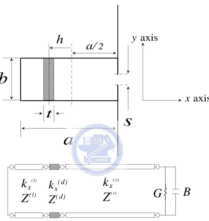
region in the waveguide. As shown in figure 3(a), inside the leaky-wave waveguide, we partition it into three sub-regions; region ‘r’ and ‘l’ in the right- and left- hand side regions, whereas the central region is filled with dielectric slab and is designated as ‘d’, which the relative dielectric constant is εs and the thickness is t. The voltage and current wave satisfy

the transmission line equations (the detailed derivations are shown in the Appendix I), which are given as follows:

) ( ) ( ( ) () () ) ( x i Z jk dx x dv i n i n i xn i n =− (19) ) ( ) ( ( ) ( ) () ) ( x v Y jk dx x di i n i n i xn i n =− (20)

Where is the propagation constant along x direction and are the corresponding characteristic impedance (admittance). They can be determined by the following equations: ) (i xn k ()( n(i)) i n Y Z 2 2 2 ) ( ε π −κ ⎟ ⎠ ⎞ ⎜ ⎝ ⎛ − = b n k k o i i xn (21) ⎪ ⎪ ⎩ ⎪⎪ ⎨ ⎧ − − = mode ; mode ; ) ( 2 2 2 2 ) ( ) ( z i xn i o i o z i o i xn o i n E k k H k k Z ε ωε κ ε κ ε ωµ (22)

, and ε_i is the relative dielectric constant in each region. Note that the propagation constant along z direction κ must remain the same in each region. In general, it is a complex

(22)

number for a leaky-wave waveguide and is to be determined in the following section of analysis.

2.3.4 Transmission Line Network Representation

B

y the electromagnetic boundary conditions, the tangential electric and magnetic field components are continuous at the interfaces between air and dielectric slab, those are the

interface planes at ⎟ ⎠ ⎞ ⎜ ⎝ ⎛₋ ₋ − = 2 t a h x and ⎟ ⎠ ⎞ ⎜ ⎝ ⎛₋ ₋ + = 2 t a h x , as given in figure 3(g). In

view of this, it is convenient to cascade these three sections of finite-length transmissions lines, as mentioned in the above section, to form a transmission line network. As for the terminations of the transmission line network, we can apply the electromagnetic boundary conditions to determine the terminations of the transmission line network. Moreover, one must make some efforts to treat the discontinuity problem, in particular for the case of waveguide opening immediate to a half space.

We look at the left-hand side of the waveguide first. Based on the electromagnetic boundary condition, the tangential electric field vanishes on the surface of PEC (perfect electric conductor) wall (x = -a). Since the tangential electric field is related to the voltage wave of the transmission line, as depicted in equation (14), it means that the voltage at the left-hand side must be zero, that is, v(-a) = 0, this shows a short-circuit termination at x = -a.

On the other hand, at the right hand side, the slit is an immediate opening to the half space. It is a problem of continuous spectra rather than the discrete modes in a closed waveguide. By the approximation formulation in Waveguide Handbook [27], we could obtain the lumped circuit elements, which contain a conductance (G) and a susceptance (B) to model the radiation and storage energy, respectively, in the vicinity of the slit discontinuity. The detailed mathematical derivation can be referred to [27] (Waveguide Handbook). With the equivalent lumped circuit at the right-hand side and shorted circuit at the left-hand side, one can obtain a complete transmission line network, where the values of conductance G and susceptance B can be referred to [26-27] and given as:

a b G Y G o 2 π = ′ = (23a) d ae a b b d a b B Y B o γ π ln ) 2 ln(csc + = ′ = (23b)

(23)

, where e = 2.718 and γ = 1.781. 2.3.5 Transverse Resonance Equation

W

ith the transmission line network representation shown in the above section, the complete network can be drawn in figure 3(h). Because the wave is propagating along a uniform waveguide along the z-direction, we are able to apply the resonance condition in the transverse plane, which is the vanishing sum of input impedances seen when looking into left and right of this reference plane (x=-c, where c is smaller than the waveguide width a). This transverse resonance equation defines the dispersion relation of the waveguide. The reference plane to perform the resonance condition can be chosen at any position within the network. However, according to our experience, to obtain an accurate dispersion root, one could choose the transverse resonance reference plane at the plane where the field strength is relatively strong. Here, both the input impedance seen when looking into left or right are functions of propagation constant κ, and the dispersion relation can be expressed as,

0 ) ( ) (κ +Z κ = Z (24)

, the symbol Z(κ) and Z(κ)represent the wave impedance seen when looking into left and right, respectively, from some arbitrary reference plane. If we choose the reference plane

as ⎟ ⎠ ⎞ ⎜ ⎝ ⎛ ₊ + − = 2 t a h

x , then the input impedance of a section of short-circuited transmission line

with length ⎟ ⎠ ⎞ ⎜ ⎝ ⎛ ₋ ₋ 2 2 t h a is given as: ( ) ⎭ ⎬ ⎫ ⎩ ⎨ ⎧ ₋ ₋ = ) 2 2 ( tan ) ( 0 () t h a k jZ Z xl l z κ (25) , where ) ( 0 ) ( 0 l x l k Z =ωµ , and 2 2 0 ) ( z l x k k k = −

(24)

Zo(l) and kx(l) represent the characteristic wave impedances and the wave propagation

constants along x direction. As for the wave impedance seen when looking to the right of the reference plane Γ − Γ + = 1 1 ) ( Z₀(r) Z κ (26) , where ⎭ ⎬ ⎫ ⎩ ⎨ ⎧ ⎟ ⎠ ⎞ ⎜ ⎝ ⎛ ₋ ₊ − ⎟⎟ ⎠ ⎞ ⎜⎜ ⎝ ⎛ + − = Γ j k a t h Z Z Z Z r x r L r L 2 2 2 exp ( ) ) ( 0 ) ( 0 ₍₂₇₎

, and the conductance G and the susceptance B have been given in equation (23)

(28)

(

₊ −1 = G jB Z_L

)

2 2 0 ) ( ) ( z r x l x k k k k = = − (29) ) ( ) ( 0 r x o r k Z = ωµ

Thus, the analytical dispersion relation is derived for solving k_z =β_z − jα_zby substituting equations (25)-(29) into equation (24). To obtain the dispersion roots in equation (24), we will use the conventional root-searching algorithm such as Newton’s method. To accelerate the root-searching process, the analytical solution of the leaky-wave waveguide free of dielectric slab, which is listed in [26], can be used as an initial point for further iteration process. The propagation constant κz in general is a complex number. Imaginary part of κz

represents the attenuation of wave propagating along the longitudinal direction of the waveguide and characterizes the power leakage from the slit into the open half plane. This shows the basic physical mechanism of the leaky-wave waveguide antenna.

2.3.6 Far Field Radiation Pattern

T

o compare the theoretical and the experimental results, we have to calculate the radiation pattern of the leaky waveguide antenna with the propagation constant which has been already found from the above derivations. Assuming that the antenna slit width is relatively small compared with the waveguide height. This makes the electric field across the antenna slit uniform in the y-direction, and propagates in the z-direction with its amplitude proportional to

(25)

exp(-jβzz)exp(-αzz). With the field distribution known inside the cavity, it is thus convenient

to use the equivalence principle to find the far field radiation pattern of the antenna concerned.

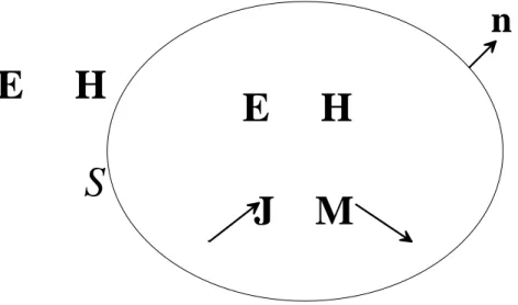
The equivalence principle states that two sets of sources producing the same field within a region of space are said to be equivalent within that region. If we are interested in the fields in a specific region, we are free to choose an equivalent set of source such that they produce the same field distribution within that region. Actual information about the original sources is not really required, equivalent sources will serve as well [38]. The equivalence principle is shown in figure 4(a) and figure 4(b). Figure 4(a) represents the sources internal to a closed surface S and free space external to S, E and H are the original electromagnetic fields all over the space. To find an equivalent source to produce equivalent electromagnetic fields outside the specific surface, it is allowed to choose the fields exist outside surface S the original field, and the field inside S the null field. To support this field, electric and magnetic surface currents, Js and Ms, must exist on S according to

(30) H Js = nˆ× n s = E× ˆ M (31)

, where is the unit vector directed outward of surface S, and E and H are the original fields over S. Since the currents are acting into the unbounded free space, we are thus able to determine the fields from the electric vector potential

nˆ

F for an equivalent magnetic source,

and the magnetic vector potential A for an equivalent electric source, they can be represented as s d r M r r e F _s s r r jko ′ ′ ′ − =

_∫

− − ′ ( ) 4 1 ' 0 πε (32) s d r J r r e A _s s r r jk o o ′ ′ ′ − =

∫

′ − − ) ( 4π _' µ (33)

where r is the observation position vector and r′ is the source position vector that is located within S.

2.3.7. The Radiation Far Field of the Antenna

A

fter the propagation constant (kz = βz-jαz) is determined by solving the dispersion root with

(26)

characteristics of this leaky-wave antenna. First, we roughly estimate the angle of radiation main beam. It can be approximated and re-state equation (5) here:

o k β θ 1 sin− ≈ (34)

In addition to the radiation angle of the main beam, we can also calculate the radiation pattern by the equivalent sources in front of the shorted circuit of slot. From the equivalence principle, the equivalent electric- and magnetic- currents Js and Ms over the slot can be

expressed as equations (30) and (31), where is the unit vector in the direction normal to the surface of the slot,

nˆ

E and H are the electric and magnetic field on the slot. Assuming the

presence of a baffle, which is an infinitely extended PEC plane, the equivalent electric current in front of this PEC plate will not radiate at all. As a result, the radiation pattern is only from the equivalent magnetic current, and is proportional the integration that is given as follows: z wd z M r r r r jk s L o ′ ′ ′ − ′ − − ≈

∫

exp( ) ( ) ϕ (35)

, r is the observation position vector, and r′ is the source position vector which is located at the z axis. And w is the width of the antenna slit, and L is the antenna slit length. We assume the field strength is uniform along the width direction of the slit. Since the magnitude of the magnetic current is proportional to exp(-jβzz)exp(-αzz), it can be

characterized as a traveling wave antenna. The parameter αL plays an important role in

(27)

Figure 1. The leaky wave above a partially open waveguide.

k

_z

=β

_z

-jα

_z

θ=sin

-1

(β

z

/k

0 )

x=z cot θ

input power

θ

x

z

Leaky Waves

(28)

Figure 2. A beam steering leaky-wave antenna for the

airborne radar of B-29 bomber implemented in WWII

by perturbation to the waveguide sidewall.

Moving waveguide side wall to change the propagation constant of TE₁₀ mode.

a

b

Antenna Slit

(29)

x=0.5a-h t a b L s 0.5a h

y

x

0.5t

Fig. 2(c) Structural parameters of the leaky wave waveguide antenna.

Figure 3(a). Structural parameters and the coordinate systems of the leaky waveguide antenna.

(30)

Figure 3(b) A slitted waveguide with

bottom plate removed.

Figure 3(c) A slitted waveguide with bottom

plate removed, then adding the flanges at input

and terminated port.

(31)

Figure 3(d) A slitted waveguide with input and

output ports.

Figure 3(e) A slitted terminated waveguide and

the placed dielectric slab on top of the metal block.

(32)

Figure 3(f) A beam steering slitted waveguide

leaky-wave antenna

(33)

Figure 3: (g) Front view of the leaky wave antenna

(h) Equivalent transmission line network

of the leaky wave antenna

k

_x

( l)

Z

( l)

k

_x

( d)

Z

( d)

k

x

( r)

Z

( r)

G

B

t

x axis

y axis

a

s

b

h

a/

2

(34)

Figure 4 (a) Original electromagnetic fields

with sources enclosed by a closed surface S.

Figure 4(b) Equivalent sources on S to

produce equivalent electromagnetic fiels.

S

Null fields inside

E H

n

E H

J M

E H

n

H

n

J

_s

=

×

n

E

M

_s

=

×

(35)

CHAPTER3. FABRICATION, MEASUREMENT SETUP, AND COMPARISON BETWEEN EXPERIMENTAL AND THEORETICAL RESULTS

3.1 Fabrication of this Antenna and the Measurement Setup

T

he proposed beam steering leaky wave antenna consists of a slitted waveguide, a moveable dielectric slab, a feed flange and a termination flange has been already shown in figure 3(a). The slitted waveguide is a Ku-band rectangular waveguide with two slits on the narrow walls of the rectangular waveguide. The slit used for the leakage of electromagnetic energy is located at the center of the narrow sidewall, at x = 0, with 1.5mm in width, and 125mm in length. Contrary to the slit for radiating the electromagnetic energy, a slit is cut in the opposite narrow sidewall of the antenna slit for moving a dielectric slab. To reduce the extra power leakage from this slit, the slit width is cut as narrow as possible. This slit is 125mm in length and 0.1mm in thickness (y=0 to 0.1 mm). A dielectric slab linearly tapered (triangular tapering with 2cm height) at both ends is mounted longitudinally on top of a thin (0.1mm thickness) rectangular (125mm length, 50mm width) plastic sheet. This sheet affects negligibly the electromagnetic field inside the waveguide. Moving this plastic sheet outside the waveguide moves the dielectric slab inside the waveguide also. This mechanism makes it possible to change the propagation constant of the dominated mode in the waveguide. Thus, the radiation angle of antenna main beam can be steered to a desired direction. Another version of mechanical setup to move the dielectric slab conveniently is to put the dielectric slab on a stationary metal block, then move the slitted waveguide (with the bottom wide plate removed also) on top of this metal block. This version of fabrication process is further demonstrated by the photographs shown from figure 3(b) to figure 3 (f). Figure 3(b) shows the slitted waveguide with its bottom plate removed, and figure 3(c) shows the flanges to add the above slitted waveguide. Figure 3(d) is already with the input port and the output port, where figure 3(e) is with an additional dielectric slab on top of the sliding metal block. Figure 3(f) is the overall beam steering antenna with the sliding metal blocks attached.

3.2 Measurement Setup

As for the experimental setup, there is a PC-based controller with a built-in data acquisition board, a vector network analyzer (VNA), a two-stage cascaded Ku-band amplifier, an

(36)

anechoic chamber equipped with a turntable and a receiving horn antenna. Test frequency is selected at 15 GHz, though this antenna can be scaled to any desired operation frequencies with a careful re-design.

In conducting experiment, the PC-based controller drives the turntable, initializes VNA, and records the measured data. Amplifiers after VNA port1 amplify the received signal to compensate system loss due to system loss, including cable and path losses. The amplified output is coupled to the antenna mounted on the turntable in the chamber. Step-motor of the turntable is with an angle resolution of 0.9 degrees. Angular error due to alignment should be controlled much smaller than 0.9 degrees. At the time the antenna is radiating and rotating on the turntable, the receiving horn antenna in the chamber delivers the received RF signal to port 2 of the VNA, where the received signal strength is measured. The acquisition board collects the data of received power versus the angular position of the turntable. A post data processor in the controller is used to plot the antenna pattern.

Far field radiation pattern should be measured in the quiet zone of the chamber with a distance greater than that of Fresnel zone (2D2/λ), where D is the maximum length of the antenna under test. That corresponds to 156cm in the test requirement for the desired test antenna. However, at the time we tested the antenna pattern, we were constrained to do measurement in a chamber with limited Fresnel zone distance of 140cm. The antenna patterns of various perturbation conditions (a combination of variant dielectric constant, dielectric slab width, and position) are measured to verify the beam steering capability of the designed antenna in this thesis.

We have also developed a chamber calibration procedure by applying the Friis’s transmission formula and the Purcell’s method for antenna gain measurement. Before conducting the antenna gain test, we are thus able to know the quietness of our chamber first. The above calibration procedure for quality control of antenna gain measurement has been shown in [40].

3.3 Comparison between experimental and theoretical results

T

o demonstrate the beam-steering capability of the leaky-wave antenna, three examples described previously were employed to verify this mechanism. The structural parameters of

(37)

the antenna have been described above in the second section. The electrical length of the antenna slit is 6.25 λ, where λ is the operation wavelength. To reduce the reflection from

the output port, the antenna was terminated with a matched load. This could further reduce the backward wave radiation.

After solving the propagation constants to the dispersion relation in equation (24), we obtained the distribution of propagation constant (kz = βz-jαz) versus shift distance (h) of the

dielectric slab. These plots were shown in figure 5-7 for case1, case2, and case3, respectively. And we summarized the results of all the three cases in figure 8. As shown in the inset in these figures, the shift distance of the moveable dielectric slab is defined as the distance from the center of the waveguide to the center of the dielectric slab. To avoid directly perturb the antenna slit, the dielectric slab was placed at the position from the central waveguide to its side wall opposite to the radiation slit, i.e. from x = -0.5a to x =-a+ 0.5t.

Since the electric field distribution of TE10 mode within the waveguide is non-uniform, the

maximum field strength is around the waveguide central part and the minimum field is at the edge. If the dielectric slab was placed around the center of the waveguide (x=-0.5a), it will strongly perturb the field distribution; and result in heavily perturbing its propagation constant (compared with the case without dielectric slab). Conversely, if the dielectric slab is positioned at the edge of the waveguide, it will (x=-a+0.5t) affect the field distribution lightly. Consequently, the normalized phase constant is close to that of the homogeneous waveguide (0.6972k_o).

In figure 5 to figure 8, the variation of normalized attenuation constant (αλ) versus the shift distance (h) for each of the previous three samples was shown, where the wavelength λ and waveguide width a are 20 mm and 15.68 mm, respectively. Since the attenuation constant determines the power leakage rate of the leaky-wave antenna, it facilitates us to estimate the radiation efficiency of this antenna. The variation of the attenuation constant will reflect in the level of power leakage. The numerical results showed that the maximum variation of attenuation constant was less than 14% for the second sample case.

Another factor affecting the radiation power is the impedance match at the antenna input port. We have measured the return loss S11 at antenna input port for each case with various shift

distances. The results showed that S11 was decreased as the shift distance was increased.

Lower return loss occurs when the dielectric slab is located near the waveguide sidewall, where the electric field is comparatively weak. On the other hand, significant influence on

(38)

the return loss was observed as the dielectric slab was moved to the center of the waveguide, since the field strength is relatively strong and being perturbed by the dielectric slab in this region. In this experiment, the measured S11 at 15GHz was less than -12dB as the shift

distance took the values from 0mm to 7mm.

The power leakage could be estimated using 1-e-2αL, where α is the leaky constant and L is the

antenna slit length. Note that, the leaky constant α depends on the slit width S of the antenna. By solving the dispersion relation in equation (24), we could obtain the phase and attenuation constant for a given slit width S. In figure 9, we calculated the function of antenna slit length (normalized to free-space wavelength) against power leakage (1-e-2αL) for the three cases with slit widths S=1mm, 1.5mm and 2mm. Note that, the dielectric slab was placed at the position with h=4mm, where the attenuation constant was of minimum value. This enables us to determine the minimum antenna length to meet a required power leakage specification. This analytical result showed that the wider the slit width the more the radiated power, which confirms the physical intuition. This figure provided us a criterion to determine the antenna slit length for a given percentage of radiation power.

To show the beam steering capability of the proposed antenna, far-field radiation pattern of the antenna at different shift distances of the dielectric slab was studied. The first dielectric slab used was the case1 dielectric sample described in the second section. The radiation patterns were measured with 1mm increment in shift distance. Results were taken, at eight shift distance values: 0mm to 7mm, as shown in figure 10 to figure 17.

The overall results in this case, both the MLTM and the experimental main beam radiation angles as functions of shift distance of the dielectric slab were summarized in figure 18. Both the angular excursion developed in this case is 9.9o according to the results.

Then, we moved to measure the far-field antenna radiation pattern at different shift distances for case 2 dielectric slab. The radiation patterns were measured with 1mm increment in shift distance, either. Results were taken, at eight shift distance values: from 0mm to 7mm, as shown in figure 19 to figure 26. We observed that the radiation angle can be continuously steered up to 23.4 degrees as the shift distance varies from 0mm to 7mm. The summarized results, both the Theoretical (MLTM) and the experimental main beam radiation angles as functions of shift distance of the dielectric slab, were collected in figure 27.

(39)

Figure 28 showed the antenna radiation patterns obtained by using the modal transmission line method (MTLM) and the experiment. Case2 dielectric slab was used, the relative dielectric constant and thickness (mm) of the dielectric slab are 2.55 and 1.62 respectively, and the shift distances h are 0, 4 and 7mm.

The last set of far-field radiation patterns of the antenna at different shift distances were studied using the case 3 dielectric slab. The radiation patterns were measured with the same

1mm increment in shift distance as the above measurements. Results were taken, at eight

shift distance values: 0mm to 7mm, as shown in figure 29 to figure 36. In case3, the theoretical (MLTM) and the experimental main beam radiation angles as functions of shift distance of the dielectric slab, were summarized in figure 37. Theoretical angular scan as shift distance varied from 0mm to 7mm was 8.1o, and the experimental one was 10.3o.

For all the theoretical and experimental main beam radiation angles of the above three cases of dielectric slabs, we have summarized the results in figure 38. Note that the main beam radiation angles while shift distances are at h=7mm were close to 45o (~sin-10.6972), because

the normalized phase constant is close to that (0.6972 ) of the homogeneous waveguide without the dielectric slab’s perturbation. Those measured radiation patterns shown in the above figures agree fairly well with those obtained by the theoretical (modal transmission line) method developed in this paper. In this radiation pattern measurement, the sweep angles φ were 0

o k

o

to 360o in an increment of 0.9o, where the angle φ was counted from z-axis, as was depicted in the inset of each figure showed the radiation angle pattern. The antenna back-lobe level was 15dB below the main-lobe, so we neglect the back-lobe and only display the radiation pattern between 0o to 90o. In addition, the antenna side lobes of the radiation patterns were significant both in the measured and the theoretical results, since the antenna slit was simply rectangular without tapering. Observable difference between these side-lobe results was probably due to the imperfect environment of our anechoic chamber. However, the trend of the measured side-lobe agreed with the theoretical one. Besides, due to the limited far-field distance (1.4 meters) of the anechoic chamber, the antenna slit length operating in the frequency in this experiment was constrained. In all the above antenna pattern measurement, numerous results have been taken, all the measured radiation patterns agreed fairly well with the theoretical results.

Figure 38 showed the variation of theoretical and experimental radiation main-beam angle versus the shift distance of the three samples of dielectric slab given in the previous section.

(40)

The theoretical radiation angle was obtained by substituting the β /k_o in figure 8 into equation (34). In figure 38, it was observed that the second case has the maximum deviation in the phase constant. It caused the beam-steering angle to be up to 23.4o. In the calculation of the theoretical phase constant, it was based on the assumption that uniform slit and dielectric slab are infinitely extended. In fact, the length of the slit and dielectric slab are finite. The discontinuities at both ends of the slit introduced some parasitic effects, such as the excitation of slot mode or cross-polarization. These effects were neglected in our theoretical analysis. Besides, precise alignment of the dielectric slab in its longitudinal direction must be carefully performed to approach the ideal case. These uncertainties may explain the differences between the theoretical and the experimental results in figure 9.

In addition to the experimental verification of an antenna design, we employed a three-dimensional electromagnetic simulation package based on Finite Integration Technique (FIT), to simulate such a leaky wave antenna. In figure39, antenna radiation pattern obtained by modal transmission line method, experimental test and Finite Integration Technique (FIT of CST Microwave Studio), using dielectric slab of case 2, and the shift distance of the dielectric slab are 0 and 7mm, respectively. We observed that when shift distance is 7mm, the angle difference of radiation main beam between the theoretical method in this paper and that of CST is 1.2o, where it is 3.7o for 0mm shift distance. Since the equivalent source on the aperture was assumed to be uniform along the width direction in our theoretical calculation, its radiation pattern may have difference compared with the FIT method. However, from the two numerical results, we found that there was only a slight difference between those two results, which proves that the assumption of uniform electric-field distribution is reasonable. Thus both these two numerical methods can be used to approve the antenna design before its fabrication. Note that, in this case, the computation resources needed in our method is considerably less than that of the FIT method.

Figure 40 depicted the variation of antenna efficiency and antenna gain against the shift distance (h) of the case 2 dielectric slab. The antenna efficiency was obtained by evaluating1−S₁₁2 − S₂₁2 , because that such a leaky-wave antenna could be regarded as a two-port device. Notably, the dielectric slab employed in this numerical simulation was assumed to be loss free. Therefore, the power loss for this two-port device was totally attributed to the radiation loss.

(41)

variation. The smallest normalized attenuation constant occurred around h=4mm, which corresponds to the lowest antenna efficiency shown in figure 40. It was evidently to know that the larger the attenuation constant, the larger amount of power leakage from the waveguide. In addition to the antenna efficiency, we also calculated the antenna gain for the same antenna in figure 40. The variation of antenna gain against shift distance (h) was plotted in this figure. Observe that the antenna gain maintained a value between 12.5 dBi and 15 dBi for changing the position of the dielectric slab. This means that the antenna gain is not so sensitive to the variation of the position of dielectric slab. It also proved the reliability of the beam-steering mechanism developed in this research.

(42)

0 1 2 3 4 5 6 7 8

Shif t Distance h (mm)

0.7 0.8 0.9 1 1.1

β/

k

0

0.04 0.08 0.12 0.16 0.2

αλ

Figure 5. Normalized phase constants and attenuation constants as

a function of shift distance using case 1 dielectric slab inside the leaky

waveguide.

s

h

(43)

0 1 2 3 4 5 6 7 8

Shif t Distance h (mm)

0.7 0.8 0.9 1 1.1

β/

k

0

0.04 0.08 0.12 0.16 0.2

αλ

Figure 6. Normalized phase constants and attenuation constants as

a function of shift distance for case 2 dielectric slab inside the leaky

waveguide.

s

h

波束可掃描之波導漏波天線設計－理論分析與天線製作量測

國

立

交

通

大

學

電信工程學系

博 士 論 文

波束可掃描之波導漏波天線設計－理論分析與

天線製作量測

A Beam Adjustable Leaky-Wave Antenna Using a Moveable

Dielectric Slab inside a Waveguide－Theoretical Analysis and

Experimental Studies

研 究 生：蕭承麒

指導教授：黃瑞彬 博士

波束可掃描之波導漏波天線設計－理論分析與天線製作量測

A Beam Adjustable Leaky-Wave Antenna Using a Moveable

Dielectric Slab inside a Waveguide－Theoretical Analysis and

Experimental Studies

研 究 生：蕭承麒 Student：Cherng Chyi Hsiao

指導教授：黃瑞彬 博士 Advisor：Dr. Ruey Bing Hwang

國 立 交 通 大 學

電信工程學系

博 士 論 文

波束可掃描之波導漏波天線設計－理論分析

與天線製作量測

A Beam Adjustable Leaky-Wave Antenna Using a Moveable

Dielectric Slab inside a Waveguide－Theoretical Analysis and

Experimental Studies

誌

謝

List of Figures

R

E

R

(

)

(

) (

)

(

)

(

)

I

(

)

(

)

∫∫

∫∫

(

)

(

)

∫∫

∫

(

)

∫∫

∫∫

(

)

(

)

∫∫

∫∫

(

)

∫∫

∫∫

(

)

∫∫

(

)

∫∫

∫∫

(

博士論文

研究生：蕭承麒

指導教授：黃瑞彬博士

研究生：蕭承麒 Student：Cherng Chyi Hsiao

指導教授：黃瑞彬博士 Advisor：Dr. Ruey Bing Hwang

國立交通大學

博士論文

₍

₎

_∫

_z

_z

_z

_x