行政院國家科學委員會專題研究計畫 成果報告
計畫類別: 個別型 計畫編號: NSC 97-2221-E-009 -108 執行期間: 97 年08 月01 日至98 年07 月31 日 執行單位: 國立交通大學工業工程與管理學系(所) 計畫主持人: 彭文理 處理方式: 本計畫可公開查詢中 華 民 國 98 年10 月30 日
考慮常態製程變異發生偏移下之製程能力調整
研究成果報告(精簡版)
Capability Adjustment for Normal Processes
with Variance Shift Consideration
W. L. Pearn and W. L. Chiang
Department of Industrial Engineering and Management, National Chiao Tung University, Taiwan
Abstract: Process capability indices (PCIs) have been proposed in the manufacturing industry to provide numerical measures on process capability, which are effective tools for quality assurance and guidance for process improvement. PCIs are calculated under the assumption that the process is stable (the process mean and variation will not change). But, in practice, the process is dynamic. If the process parameters have a small shift, the control chart not be able to detect immediately. PCIs, in this case, will overestimate the true process capability. For this reason, the PCIs have to be adjusted. Bothe (2002) provided the adjustment method for normal processes with mean shift. In practice, the variance could change as well. In this project, we provide capability adjustment for normal processes with standard deviation change. The magnitude of adjustment is correlated to the detection power of the control chart used. We first investigate the detection powers of 2
S and S control charts under various sample
subgroup sizes, and derive the magnitude of the adjustment. We add the adjustment to the formula of process capability index Cpkfor normal processes. For illustration purpose, an application example is presented.
Keywords: Dynamic Cpk, Variance change, Process capability index, Normal distribution, Chi-square distribution, S2 control chart, S control chart
1. Introduction
Process capability indices are important for any successful quality improvement activities and quality program implementation. They have been the focus of recent research in quality assurance and process capability analysis. Process capability indices establish the relationship between the actual performance and the manufacturing specifications, which provide management with a single-number summary of the process capability in a format that is easy to use and understand. Thus, the capability indices have been widely used in the manufacturing industry. The two basic, most commonly used indices for assessing process potential and performance, Cpand Cpkwere discussed in Kane
(1986). The more advanced index Cpm was formalized by Chan et al. (1988) to
offset the weakness of the first-generation indices, taking the target value of the process into account. The third-generation index Cpmkwas introduced by Pearn et
al.(1992), which is more restrictive regarding to process mean deviation from the target value than the other two indices. Those PCIs defined as:
2 2 , m in , , 6 3 3 6 ( ) p pk pm U SL LSL U SL LSL U SL LSL C C C T 2 2 2 2 m in , , 3 ( ) 3 ( ) pmk USL LSL C T T
where USL and LSL are the upper and lower specification limits, respectively. is the process mean, is the process standard deviation, and T is the target value. The index Cp simply measures the spread of the specifications relative to
the six-sigma spread in the process. The magnitude of Cpkrelative to Cpis a direct
measure of how off-center the process is operating. For a Cpk level of 1,
statistically one would expectthatthe product’s fraction ofdefectives is no more than 2700 parts per million (PPM) fall outside the specification limits. At Cpk
=1.33, the defect rate drops to 66 PPM. To attain less than 0.544 PPM defect rate, a Cpk level of 1.67 is required. At a Cpk level of 2.0, the defective rate reduced to
0.002 PPM. Note that the PCIs are absolutely critical to the assumptions that the process is stable and their usual interpretation is based on normal distribution of process output. Unfortunately, it is fairly common practice to compute a PCI from a sample or historical process data without checking whether the process is under those assumptions. If they are not valid, then the statements about the expected process fallout attributed to a particular value of PCIs may be seriously in error. In this situation, we need to modify the PCIs to have a more accurate calculation and interpretation.
However, no process is ever truly stable. The concept of the six-sigma process is one way to accommodate the process behavior. The six-sigma quality improvement process was proposed by Motorola Inc. in 1986. Through years of process experience and data collection, Motorola Inc. has determined that processes will drift over time. Almost since that time, followers of this philosophy asserted that adding a shift to the average before estimating process capability is necessary. The range of shift typically falls between 1.4 and 1.6. Acknowledging that processes will experience shifts in of various magnitudes. To have proper and to improve the process performance, adjusted PCIs are proposed. Bothe (2002) has provided a statistical reason to this issue, modifying the capability assessment. Since the processes are dynamic. The also undergoes some changes. In this project, we provide capability adjustment for normal processes with standard deviation change. The magnitude of adjustment is correlated to the detection power of the control chart used. We first investigate the detection powers of 2
S and S control charts under various sample subgroup sizes, and derive the magnitude of the adjustment. We add the adjustment to the formula of process capability index Cpk for normal processes.
For illustration purpose, an application example is presented.
2. Literature Review
The six-sigma advocates claim it is necessary to add a 1.5 shift to the average for most processes, with only personal experiences and three dated empirical studies as justification (see Bender (1975), Evans (1975), Gilson (1951)). In this chapter,we provide Bothe’s statisticalrationale regarding this issue.The data in Bothe’s study was assumed to be close to normaldistributions.For the process output having non-normal distributions, we also conduct some studies here.
2.1. Process Capability Adjustment for Normal Processes with Mean Shift
Shewhart control charts are very useful in phase I implementation of SPC, where the process is likely to be out of control and experiencing assignable
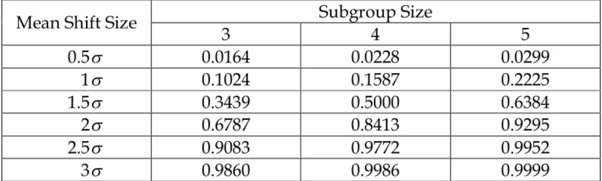
causes that result in large shifts in the monitored parameters. Nevertheless, a major disadvantage of a Shewhart control chart is that it uses only the information about the process contained in the last sample observation and it ignores any information given by the entire sequence of points. This feature makes the Shewhart control chart relatively insensitive to small process shift. This potentially makes Shewhart control charts less useful in phase II monitoring problems, where the process tends to operate in control, reliable estimates of the process parameters (such as the mean and standard deviation) are available, and assignable causes do not typically result in large process upsets or disturbances. This is demonstrated in Table 1, displays the probabilities of detecting changes in versus subgroup size for shift 0.5(0.1)3 with n 3, 4 and 5 . The probabilities of detecting small shifts in are close to zero. As the size of the shift increases, so does the detection power of the X control chart to detect it, with sample subgroup sizes n 3, 4 and 5 eventually close to 100 percent for shifts in excess of 3.
Table 1. Probabilities of detection the mean shift versus subgroup size n. Subgroup Size
Mean Shift Size
3 4 5 0.5 0.0164 0.0228 0.0299 1 0.1024 0.1587 0.2225 1.5 0.3439 0.5000 0.6384 2 0.6787 0.8413 0.9295 2.5 0.9083 0.9772 0.9952 3 0.9860 0.9986 0.9999
In studying the properties of control charts, the emphasis has been on determining the detection power and ARL (Average Run Length) of the chart. The ARL of a chart is the expected number of samples to be taken before the chart detects a shift in the process characteristic. The ARL should be large when there has been no change in the process, but the ARL should be small when the process having undergone a change. The value of the ARL is depending on the purpose being studied. For any Shewshart control chart, we have noted that the
ARL can also be expressed as
0 1 , ARL
for the in-control false alarm ARL0 and 1 1 , 1 ARL
for the out-of-control ARL1, where is the probability of detecting a shift when none has occurred, and is the probability of failing to detect a real shift in process characteristic. In general, we set ARL1 in most applications.2 Therefore, the detection power is
1 1 1 D etection power 1 0.5, 2 ARL
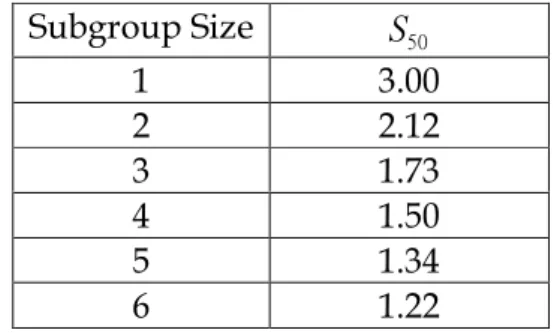
that is, the probability of the control chart to detect the small shift immediately within two samples is 50 percent. By this idea, Bothe set the detection power to be 50 percent and computed the several magnitude of adjustments for various sample subgroup sizes. The results are shown in Table 2, which displays shift sizes that have a 50 percent chance of failing to detect the change in , which we refer to as , for various sample subgroup sizes from 1 to 6.
Table 2. S50 values for normal distribution with various subgroup sizes. Subgroup Size S50 1 3.00 2 2.12 3 1.73 4 1.50 5 1.34 6 1.22
Because shifts ranging in size from 0 up to S50 are likely to remain undetected, a conservative approach is to assume that every missed shift is as large as S50. And Bothe made the modifications into the Cpkformula, called the
dynamic Cpk, defined as follow:
Dynamic Cpk 50 50 ( ) ( ) min , . 3 3 USL S S LSL
2.2. Process Capability Adjustment for Non-normal Processes with Mean Shift
However, for the majority of cases, normal data seem impossible to be found in real-world situations. Pyzdek (1992) has mentioned the distributions of certain chemical processes such as zinc plating thickness of a hot-dip galvanizing process are very quite often skewed. Choi (1996) presents an example of a skewed distribution in the “active area” shaping stage ofthe wafer’s production processes. The abundance of outputs from skewed distributions, the censoring effects induced by the finite precision of actual measurements, stratification, etc., makes the normal assumption often unreasonable. Thus, there should be more concern about how the indexes are applied.
In the recent years, several approaches to dealing with problems of PCIs for the non-normal populations have been suggested (see e.g. pal (2005), Ding (2004), Pearn and Chen (1997), Kotz and Lovelace (1998), Somerville and Montgomery (1996), Kocherlakota et al.(1992)). One approach to dealing with this situation is to transform the data so that in the new, transformed metric the data have normal distribution appearance. There are various graphical and analytical approaches to selecting a transformation, such as Box-Cox power transformation and Johnson’s transformations. And some authors replaced the unknown distribution by a known three or four-parameter distribution. Examples include Clements (1989), Franklin and Wasserman (1992), Shore (1998) and Polansky (1998).
There have also been attempts to modify the usual capability indices so that they are appropriate for both normal and non-normal distributions. The general
idea is to use appropriate quantiles of the process distribution, x0.00135and x0.99865,
to define a quantile-based PCIs. Good discussions of these approaches are in Kotz and Lovelace (1998).
Hsu et al. (2007) examine Bothe’s study and find the detection power was less than 0.5 when data came from Gamma distributions,showing thatBothe’s statistical rationales are inadequate when we had Gamma processes. Then, Hsu et al. (2007) calculate the magnitude of adjustments which called AS50 under various sample subgroup sizes n and Gamma parameter N , with power fixed to 0.5. Table 3 displays the magnitude of adjustments AS50 which Hsu et al. provided and data come from G am ma( ,1)N with various values of N =1(1)10 and n=2(1)6.
Table 3. AS50 values for various subgroup sizes n and various of Gamma( ,1)N .
n 1 2 3 4 5 6 7 8 9 10 N(0,1) 2 3.611 3.185 2.992 2.876 2.797 2.738 2.692 2.655 2.625 2.599 2.12 3 2.732 2.443 2.313 2.236 2.182 2.143 2.113 2.088 2.067 2.050 1.73 4 2.252 2.034 1.936 1.878 1.838 1.808 1.785 1.767 1.752 1.738 1.50 5 1.944 1.769 1.690 1.644 1.612 1.588 1.570 1.555 1.543 1.532 1.34 6 1.727 1.581 1.515 1.476 1.450 1.430 1.415 1.403 1.392 1.384 1.22 7 1.565 1.439 1.383 1.350 1.327 1.310 1.297 1.286 1.278 1.270 1.13 8 1.438 1.328 1.279 1.249 1.229 1.215 1.203 1.194 1.186 1.180 1.06 9 1.336 1.237 1.194 1.168 1.150 1.137 1.127 1.118 1.112 1.106 1.00 10 1.251 1.162 1.123 1.100 1.084 1.072 1.063 1.055 1.049 1.044 0.95 Then, Hsu et al. (2007) used the quantile estimation to modify Cpkas:
0.99865 0.00135 m in , m edian m edian m in , . m edian m edian pk pu pl C C C USL LSL x xTo consider the undetected process mean shift, Hsu et al. (2007) obtained Dynamic Cpkindex for non-normal processes by modifying Bothe’s Dynamic Cpk:
Dynamic Cpk 0.5 50 0.5 50 0.99865 0.5 0.5 0.00135 ( ) ( ) m in USL F AS , F AS LSL . F F F F 3. Normal Process
Normal process is applicable in many fields. Many phenomena generate random variables with probability distributions that are very well approximated by normal distribution. In this chapter, we introduce normal distribution and the sampling distributions of the statistics.
3.1. Normal Distribution
variable is normal distribution. There are three reasons why normal distribution plays a very important role in both the theory and application of statistics. First, normal distributions are good descriptions for some distributions of real data. Distributions that are often close to normal include scores on tests taken by many people, repeated careful measurements of the same quantity, and characteristics of biological populations. Second, normal distributions are good approximations to the results of many kinds of chance outcomes, such as the proportion of heads in many tosses of a coin. Third, we will see that many statistical inference procedures based on normal distributions work well for other roughly symmetric distributions. Normal distribution is also referred to as the Gaussian distribution.
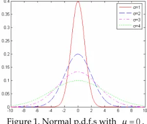
Random variables with different means and variances can be modeled by normal probability density functions with appropriate choices of the center and width of the curve. The exact density curve for a particular normal distribution is described by giving its mean and its standard deviation . The value of
( )
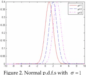
E X determines the center of the probability density function. Changing without changing moves the normal curve along the horizontal axis without changing its spread. The value of 2
( )
V X determines the width, controlling the spread of the normal curve.
The probability density function of the normal random variable X with mean and standard deviation is given by
2 1 2 1 ( ) , , , 0. 2 x f x e x (1)
This distribution is commonly denoted by 2 ( , ) N . The cumulative distribution function is
2 1 2 1 ( ) . 2 x a F a P x a e dx (2)Since the mean is the location parameter, and the standard deviation is the scale parameter. See Figures 1 and 2. The visual appearance of normal distribution is a symmetric, single-peaked, and bell-shaped curve.
Figure 2. Normal p.d.f.s with 1.
3.2. Statistics and Sampling Distributions
An important sampling distribution defined in terms of normal distribution is the Chi-square or 2 distribution. Let
1, 2,..., n
X X X are normally and
independently distributed random variables with N (0,1). Then the random variable 2 1 n i i Y X
(3)is called the Chi-square distribution with degrees of freedom (df) n , and its probability density function is given by
/ 2 ( / 2 ) 1 / 2 1 ( ) , y 0, 0. 2 ( / 2) y n n f y e y n n (4)
The mean and variance are given, respective, by , n (5) and 2 2 ,n (6)
The Chi-square random variable with df n is denoted by 2
n
. The Chi-square distribution is a continuous asymmetrical theoretical probability distribution. The Chi-square value must fall within the range 2
0 , and thus can never be a negative number. The coefficient of skewness and kurtosis of Chi-square are given by
1 2 = 2 , n (7) and 2 12 3 , n (8)
Table 4 presents the values of skewness and kurtosis of the Chi-square distribution. It is reveal that 2
a
is stochastically larger than 2
b
for a b .
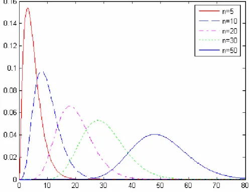
Plots in Figure 3 indicate that, the Chi-square distribution is a right-tail distribution and it can be found that for large degrees of freedom n , the Chi-square distribution is symmetric about its mean.
Figure 3. Chi-square distribution with various degrees of freedom n . The Chi-square distribution is also called the variance distribution by some authors, because the variance of a random sample from normal distribution follows a Chi-square distribution. Specifically, if X X1, 2,...,Xn is a random sample from an
2 ( , ) N distribution. Then the probability density function of the sample
Table 4. Values of skewness and kurtosis for various Chi-square distributions.
Distribution Skewness Kurtosis
N(0,1) 0.0000 3.0000 2 5 1.2649 5.4000 2 10 0.8944 4.2000 2 20 0.6325 3.6000 2 30 0.5164 3.4000 2 40 0.4472 3.3000 2 50 0.4000 3.2400
variance 2 2 1 ( ) / 1 n i i S X X n
is 2 3 ( 1) / 2 2 2 2 2 ( 1)/ 2 1 ( 1) ( 1) ( ) , u 0 1 2 ( ) 2 n n u n n u n f u s e n (9)and the sampling distribution of the sample standard deviation 2 1 ( ) / 1 n i i S X X n
is 2 2 3 ( 1) / 2 2 2 2 2 ( 1)/ 2 1 ( 1) ( 1) ( ) 2 , v 0 1 2 ( ) 2 n n v n n v n f v s e v n (10)3.3. Point Estimation of Normal Processes Parameters
Suppose that the variance and standard deviation2 of normal distribution are both unknown. If a random sample of n observations is taken, then the sample variance S2 and sample standard deviation
4 /
S c are point estimators of the population variance 2 and population standard deviation , respectively. It can be shown that
1/ 2 2 2 4 2 ( / 2) ( ) and ( ) . 1 [( 1) / 2] n E S E S c n n
Furthermore, the standard deviation of S is 2 4 1 C
.
4. Process Variance Change Investigation for Normal Processes Using S2 Control Chart
The major purpose of individuals control chart is assisting on identifying shifts and drifts in processes and it is easily to be implemented. But some assumptions should be satisfied before control charts are used. The assumptions include that the process must in stationary. In practice, process is not stable. Due to above-mentioned statements, the steps in calculating the probabilities for catching various magnitude of change under various sample subgroup sizes n of
2
S control chart are as followings.
4.1. Detection Power of 2
S Control Chart for Normal Processes
STEP 1: Construct the limits. The parameters of the 2
S control chart are
2 2 0.00135, 1 2 2 2 0.99865, 1 U CL , 1 Center line , LCL , 1 n n S n S S n (11)
where 2 0.00135,n 1
and 2
0.99865,n 1
denote the 0.00135 and 0.99865 percentage points of the Chi-square distribution with n-1 degrees of freedom, and the statistic 2
S is an average sample variance obtained from the analysis of preliminary data.
STEP 2: Consider the detection power for an S2 control chart. If changes from the in-control value to another value k0. The probability of detecting this change is
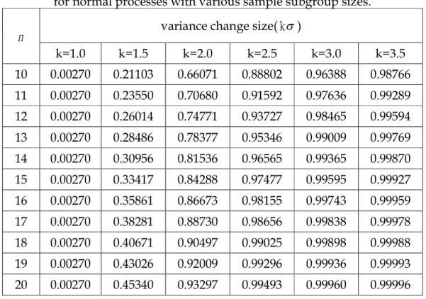
│ │ 2 1 0 2 1 0 D etection power 1 1 ( ) 1 ( UCL ( ) ). LCL P LCL S UCL k P f u s du k (12) where f u( ) denotes the sampling distribution of the sample variance and 1 is the standard deviation after variance change (0 is the standard deviation of the original process).Table 5 presents the detection power with various magnitude of standard deviation change when data come from normal distribution under various sample subgroup sizes n 10(1)20 . For an S2 control chart with sample subgroup size n , changes greater than10 20 have more than a 66.1 percent chance of detecting the standard deviation changes. However, the chance of catching a 1.50 change being only 21.1 percent. Such low probabilities mean that small changes to standard deviation may come and go, without us ever being aware they have negatively impacted our process.
Table 5. The detection power of the S2 control chart for normal processes with various sample subgroup sizes.
variance change size( k) n k=1.0 k=1.5 k=2.0 k=2.5 k=3.0 k=3.5 10 0.00270 0.21103 0.66071 0.88802 0.96388 0.98766 11 0.00270 0.23550 0.70680 0.91592 0.97636 0.99289 12 0.00270 0.26014 0.74771 0.93727 0.98465 0.99594 13 0.00270 0.28486 0.78377 0.95346 0.99009 0.99769 14 0.00270 0.30956 0.81536 0.96565 0.99365 0.99870 15 0.00270 0.33417 0.84288 0.97477 0.99595 0.99927 16 0.00270 0.35861 0.86673 0.98155 0.99743 0.99959 17 0.00270 0.38281 0.88730 0.98656 0.99838 0.99978 18 0.00270 0.40671 0.90497 0.99025 0.99898 0.99988 19 0.00270 0.43026 0.92009 0.99296 0.99936 0.99993 20 0.00270 0.45340 0.93297 0.99493 0.99960 0.99996
One way to improve the odds of catching small changes in is to increase the sample subgroup size. The chance of detecting a 33.4 percent when n , to15 almost 43 percent when n . However, this chance falls to only 21.1 percent if19
10 n .
4.2. Modified Variance Adjustments for Normal Processes
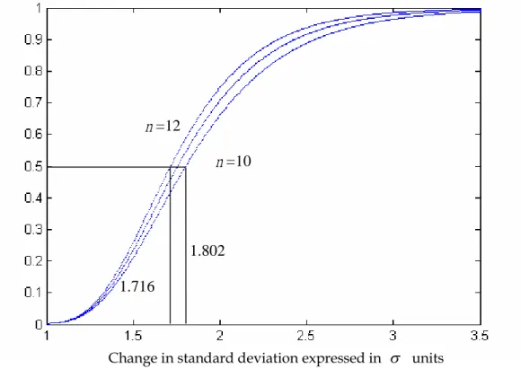
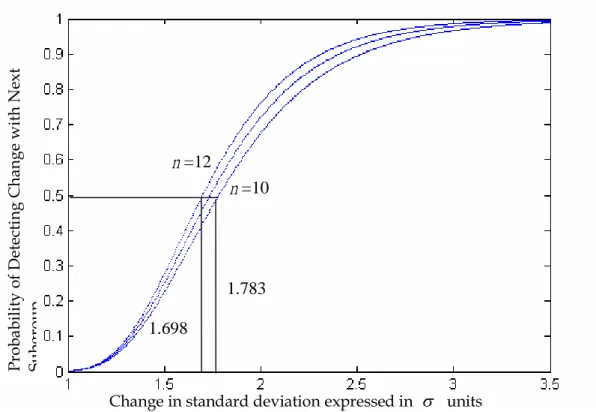
The probabilities in Table 5 are plotted on the graph displayed in Figure 4, with one curve for each sample subgroup size. Those curves are power curves, these lines portray the chances of detecting a change in standard deviation of a given size (expressed in units on the horizontal axis). For small change in standard deviation, all three curves are close to zero. As the size of the change increases, so does the detection power of the chart, with all three curves eventually leveling off close to 100% for shifts exceeding 3.5. The horizontal lines in Figure 4 show that there is a 50% chance of missing a 1.72 change in standard deviation when n 12 for 2
S control chart, whereas must move by 1.80 to have this same probability when n .10
Figure 4. Power curves of 2
S control chart for subgroup sizes 10, 11 and 12. The necessary adjustment due to the undetected standard deviation change is called ASpower which is the magnitude of change we need to adjust based on
designated detection power and process data come from normal distributions. We develop a Matlab program to determine the adjustment ASpower by setting
the desired detection power and the sample subgroup size n. Generally, the sample subgroup size of 2
S and S control charts is moderately
n=12 n=10 1.802 1.716 Pr ob ab ili ty of D et ec tin g C ha ng e w it h N ex tS ub gr ou p
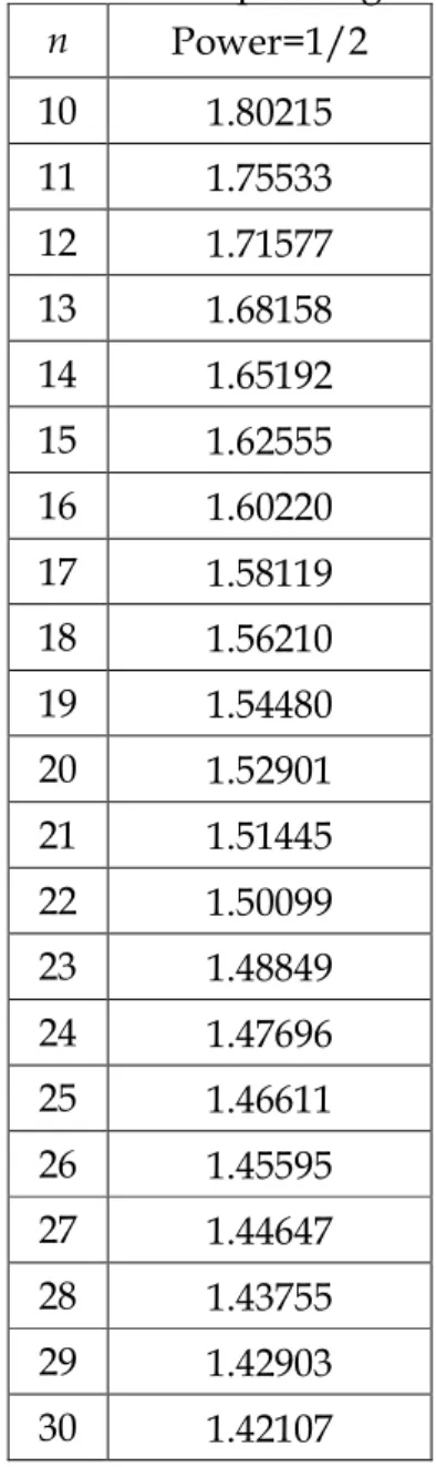
large( n 10 or 12 ). If we set detection power 1/ 2 and n 10(1)30 . The magnitude of adjustment AS1/ 2 based on
2
S control chart is shown from Table 6. Temporary movements in smaller than ASpower are more than likely to
be missed by a control chart. We also provide the ASpower values of
2
S control charts (See Appendix A) for detection power 1/ 3, 1/ 4 and 1/ 5 versus various sample subgroup sizes n 2(1)30.
4.3. Modified Process Capability Cpk for Normal Processes
Acknowledging that processes will experience change in various magnitude of variance, and knowing that not all of these will be discovered, some allowance for them must be made when estimating outgoing quality so customers are not disappointed. Because changes ranging in size from 0 up to ASpower are
Table 6. ASpower values of
2
S control chart for various sample subgroup sizes.
n Power=1/2 10 1.80215 11 1.75533 12 1.71577 13 1.68158 14 1.65192 15 1.62555 16 1.60220 17 1.58119 18 1.56210 19 1.54480 20 1.52901 21 1.51445 22 1.50099 23 1.48849 24 1.47696 25 1.46611 26 1.45595 27 1.44647 28 1.43755 29 1.42903 30 1.42107
likely to remain undetected (larger moves should be caught by the chart), a conservative approach is to assume that every missed change is as large as
power
A S .
Since changes can move standard deviation larger or smaller, in place of using ˆ for the process variance when estimating capability, ˆ multiplied by
power
AS is a conservative way to evaluate the process capability. The adjustment is incorporated into the Cpk formula, which we refer to as “dynamic” Cpk
index, by making the following modifications: ˆ m in , ˆ 3 pk power USL C AS ˆ . ˆ 3 power LSL AS (13)
By including an adjustment in this assessment for undetected shifts in variance, the estimate of capability will decrease and the expected total number nonconforming parts will increase. To illustrates the use of dynamic Cpk index,
setting the detection power 0.5 of 2
S control chart. Then A Spower 1.63 (see Table 6) when n 15 from normal distribution. Factoring in the possibility missing changes in of up to 1.63 drops the Cpk index.
5. Process Variance Change Investigation for Normal Processes Using S Control Chart
Most quality engineers use either S2 control chart or the S control chart to monitor process variability. In this chapter, we exhibit the detection powers of S control chart by using the sampling distribution of S to find the adjustment for normal processes with standard deviations change.
5.1. Detection Power of S Control Chart for Normal Processes
Setting up and operating control charts for S requires about the same sequence of steps as those for S2 control chart, except that for each sample we must calculate the sample standard deviation S ,
1 1 . m i i S S m (14)STEP 1: Construct the limits. The statistic S c/ 4 is an unbiased estimator of
. Therefore, the parameters of the S control chart would be 4 3 U CL , Center line , LCL . B S S B S (15) We usually define the constants
2 3 4 4 2 4 4 4 3 1 1 , 3 1 1 . B c c B c c (16)
Note that this control chart is defined with three-sigma control chart limits.
STEP 2: Consider the detection power for an S control chart. If the standard deviation changes from the in-control value to another value k0. The probability of detecting this change is
│ │ 1 0 1 0 D etection pow er 1 1 ( ) 1 ( UCL ( ) ), LCL P LCL S UCL k P f v s dv k (17)where f v( ) denotes the sampling distribution of the sample standard deviation and 1 is the standard deviation after variance change (0 is the standard deviation of the original process).
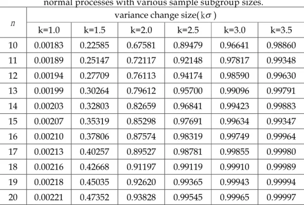
Table 7 displays the detection power of S control chart with various magnitude of standard deviation change ( k) when data come from normal distribution under various sample subgroup sizes n10(1)20.
5.2. Modified Variance Adjustments for Normal Processes
Figure 5 depicts the power curves of S control chart. Those lines portray the probability of detecting a change in standard deviation of a given size (expressed in units on the horizontal axis). For small change in standard deviation, all three curves are close to zero. As the size of the change increases, so does the power of the chart to detect it, with all three curves eventually leveling off close to 100% for shifts in excess of 3.5.
The horizontal in Figure 5 show that there is a 50% chance of missing a Table 7. The detection power of the S control chartfor
normal processes with various sample subgroup sizes. variance change size( k)
n k=1.0 k=1.5 k=2.0 k=2.5 k=3.0 k=3.5 10 0.00183 0.22585 0.67581 0.89479 0.96641 0.98860 11 0.00189 0.25147 0.72117 0.92148 0.97817 0.99348 12 0.00194 0.27709 0.76113 0.94174 0.98590 0.99630 13 0.00199 0.30264 0.79612 0.95700 0.99096 0.99791 14 0.00203 0.32803 0.82659 0.96841 0.99423 0.99883 15 0.00207 0.35319 0.85298 0.97691 0.99634 0.99347 16 0.00210 0.37806 0.87574 0.98319 0.99749 0.99964 17 0.00213 0.40257 0.89527 0.98781 0.99855 0.99980 18 0.00216 0.42668 0.91197 0.99119 0.99910 0.99989 19 0.00218 0.45035 0.92620 0.99365 0.99943 0.99994 20 0.00221 0.47352 0.93828 0.99545 0.99965 0.99997
1.70 change in standard deviation when n 12 for S control chart, whereas standard deviation must change by 1.78 to have this same probability when
10 n .
Figure 5. Power curves of S control chart for sample subgroup sizes 10, 11 and 12.
The undetected standard deviation change adjustment is called ASpower
which is the magnitude of change we need to adjust based on designated detection power and process data come from normal distribution. We develop a Matlab program to determine the adjustment ASpower by setting the desired
detection power and the sample subgroup size n. For example, if we set detection power=1/2 and n 10(1)30. The magnitude of adjustment AS1/ 2 based on S control chart is shown from Table 8.
We also provide the ASpower values of S control chart (See Appendix B) for
detection power 1/ 3, 1/ 4 and 1/ 5 versus various sample subgroup sizes 2(1)30
n .
Table 8. ASpower values of S control
charts for various sample subgroup sizes. power1/ 2 n S control chart 10 1.78265 11 1.73679 n=12 n=10 1.783 1.698 Pr ob ab ili ty of D et ec ti ng C ha ng e w it h N ex t Su bg ro up
6. Application
In the previous chapter we presented the statistical reason for the magnitude of adjustment for 2
S and S control charts. We now illustrate the application of the dynamic Cpk to estimate process capability.
Because of advantages such as long lifetime, low power consumption, and no mercury containing, Light Emitting Didoes (LEDs) are widely used in a variety of general-purpose illumination applications. For indoor illumination, there are two different approaches for generating white light with LEDs. One way is combining a blue or UV LEDs with a down conversion phosphor, and the other way to obtain white light is mix the monochromatic LEDs with different colors. The later approach seems a better way to generate white light for indoor illumination. Figure 6 illustrates the red, green and blue (RGB) LEDs in one package. For RGB LEDs, or the white light mixed by more than three LEDs, the color rendering and luminous efficiency depend on the choice of the individual peak wavelengths of the LEDs, which will lead to very different color rendering and luminous efficiency. So the optimization of the white light formed by more than two LEDs can achieve a maximum of certain luminous efficiency and
12 1.69806 13 1.66483 14 1.63585 15 1.61031 16 1.58751 17 1.56705 18 1.54865 19 1.53175 20 1.51637 21 1.50237 22 1.48932 23 1.47723 24 1.46597 25 1.45547 26 1.44565 27 1.43645 28 1.42780 29 1.41956 30 1.41187
color-rendering index (CRI). To make sure the optical properties are acceptable to customers, the wavelengths we choose with highest luminous efficiency at that time are in blue 455-480 nanometer (nm), green 510-535 nm and red 610-630nm regions.
To illustrate the use of the dynamic Cpk to estimate process capability.
Consider Table 9, which presents a part of historical data of wavelength for blue LED collected from the factory. The proposed specifications on wavelength for blue LED are USL = 480nm and LSL = 455nm, respectively. From Figure 7, note that the data lie nearly along a straight line, implying that the distribution of wavelength is normal distribution. Furthermore, Figure 8 shows the shape of the histogram implies that the distribution of wavelength is approximately normal distribution.
Table 9. The 100 observations are collected from the historical data. 463.029 466.841 463.560 462.841 467.381 465.297 463.411 462.623 463.485 470.220 464.694 463.413 464.895 467.947 465.504 462.441 464.557 465.835 463.000 464.413 467.604 464.955 464.273 464.092 466.544 464.966 465.614 463.900 463.886 461.244 466.180 467.328 464.921 468.563 469.098 463.424 466.368 464.616 465.178 467.435 463.558 461.149 462.894 462.622 462.299 465.692 466.534 467.844 462.526 463.526 465.235 466.785 465.970 468.819 467.950 469.066 466.400 467.818 469.262 465.854 464.395 467.882 463.905 468.597 465.865 469.868 465.720 462.539 462.237 463.927 468.319 463.519 466.777 464.530 465.501 460.721 464.672 465.091 464.562 466.508 461.303 459.612 463.336 465.677 463.599 463.738 466.041 464.804 463.741 462.794 464.591 465.257 460.581 462.849 464.592 465.020 463.700 467.385 464.017 462.681
Figure 6. The RGB LEDs.
Figure 8. Histogram plot of the historical data.
The parameters and of this normal process could be estimated from the historical data, giving ˆ 464.98 and ˆ 2.20 . Cpk can be calculated as
follows: ˆ m in , ˆ 3 pk USL C ˆ ˆ 3 LSL 480 465 465 455 min , 3(2.20) 3(2.20)
min 2.27,1.52 1.52. Under the assumption of a stationary standard deviation. By including an adjustment in this assessment for undetected change in standard deviation, the estimate of capability will decrease and the expected total number of nonconforming parts will increase. From Table 6, A S1/ 2 of
2
S control chart is 1.80 when n . Compared10 Cpk to the value of the following index:
ˆ D ynam ic m in , ˆ 3 pk power USL C AS ˆ ˆ 3 power LSL AS 480 465 465 455 min , 3(2.20)(1.80) 3(2.20)(1.80)
min 1.26, 0.84 0.84. We can see that the value of the dynamic Cpk is much smaller. By increasing the
sample subgroup size n, a change in has a higher probability to be detected. For example, if n , the15 A S1/ 2 would be 1.63 for normal distribution and
ˆ D ynam ic m in , ˆ 3 pk power USL C AS ˆ ˆ 3 power LSL AS 480 465 465 455 min , 3(2.20)(1.63) 3(2.20)(1.63)
min 1.39, 0.93 0.93. Changing sample subgroup size n from 10 to 15 increases the dynamic Cpk
index value from 0.84 to 0.93.
7. Conclusion
In Bothe’s study, the author provided the statistical rationale for adjusting estimates of process capability by including a possible shift in . But the case of standard deviation change occurs frequently in practice. This project has considered the problem for adjusting estimates of process capability by including a change in when the process output has normal distribution. We use a Matlab program (available on request) to compute the standard deviation change adjustments based on the detection power is 1/2(ARL1 ), 1/3(2 ARL1 ),3 1/4(ARL1 ), 1/5(4 ARL1 ) percent for data come from normal distribution5 with various values of n 2(1)30. The adjustments are incorporated into the
pk
C formula, which we refer to as the “dynamic”Cpk index. It has proven to
be a useful way for the engineers/practitioners to access process performance. A real-world application on LED production plant is investigated and presented to illustrate the applicability of the proposed approach.
References
1. Bender, A., Statistical Tolerancing as it Relates to Quality Control and the Designer, Automotive Division Newsletter of ASQC, 1975.
2. Bothe, D. R. (2002). Statistical reason for the 1.5 shift. Quality Engineering, 14(3), 479-487.
3. Chan, L. K., Cheng, S. W. and Spiring, F. A. (1988). A new measure of process capability Cpm. Journal of Quality Technology, 20(3), 162-175.
4. Choi, K. C., Nam, K. H. and Park, D. H. (1996). Estimation of capability index based on bootstrap method. Microelectronics Reliability, 36(9), 141-153. 5. Clements, J. A. (1989). Process capability Calculations for non-normal
distributions. Quality Progress, September, 95-100.
6. Ding, J. (2004), a method of estimating the process capability index from the first four moments of non-normal data. Quality and Reliability Engineering International, 20, 787-805.
7. Douglas C. Montgomery (2005). Introduction to Statistical Quality Control, Fifth Edition, 339-343.
8. Evans, D. H., Statistical Tolerancing: The State of the Art, Part III: Shifts and Drifts, Jorunal of Quality and Technology, April 175, pp. 72-76.
9. Franklin, L. A. and Wasserman, G.S. (1992). Bootstrap lower confidence limits for capability indices. Journal of Quality Technology, 7(2), 72-76. 10. Gilson, J., A New Approach to Engineering Tolerances, Machinery Publishing
Co., London, England, 1951.
11. Hsu, Y. C., Pearn, W. L. and Wu, P. C. (2007). Capability adjustment for gamma processes with mean shift consideration in implementing Six Sigma program. European Journal of Operational Research, In Press, Corrected Proof, Available online 25 July.
12. Krishnamoorthy K. (2006). Handbook of Statistical Distributions with Applications, 119-155.
13. Kane, V. E. (1986) Process capability indices. Journal of Quality Technology, 18(1), 41-52.
14. Kocherlakota, S., Kocherlakota, K. and Kirmani, S. N. U. A. (1992) process capability index under non-normality. International Journal of Mathematical Statistics, 1(2), 175-210.
15. Kotz, S. and Lovelace, C. R. (1998). Process Capability Indices in Theory and Pratice, Arnold, London, U. K.
16. Lewis Vanbrackle, and G. David Williamson (1999). A Study of The Average Run Length Characteristics of The National Notifiable Diseases Surveillance System. Statistics in Medicine, 3309-3319.
17. Pal, S. (2005). Evaluation of non-normal process capability indices using generalized lambda distribution. Quality Engineering, 17, 77-85.
18. Pearn, W. L., and Chen, K. S. (1997). Capability indices for non-normal distributions with an application in electrolytic capacitor manufacturing. Microelectronics and Reliability, 37(12), 1853-1858.
19. Pearn, W. L., Kotz, S. and Johnson, N. L. (1992). Distributional and inferential properties of process capability indices. Journal of Quality Technology, 24(4), 216-233.
20. Polansky, A. M. (1998). A new approach to analyzing non-normal quality data with application to process capability analysis. International Journal of Production Research, 36(7), 1917-1933.
21. Pyzdek, T. (1992). Process capability analysis using personal computers. Quality Engineering, 4(3), 419-440.
22. Shore, H. (1998). A new approach to analyzing non-normal quality data with application to process capability analysis. International Journal of Production Research, 36(7), 1917-1933.
23. Somerville, S. E. and Montgomery, D. C. (1996). Process capability indices and non-normal distributions. Quality Engineering, 9(2), 305-316.
Appendix A.
AS
power for Normal Processes with Variance Change Using 2 S Control Chart Detection Power n 1/3 1/4 1/5 10 1.62857 1.54233 1.48767 11 1.59479 1.51459 1.46323 12 1.56595 1.49055 1.44235 13 1.54095 1.46982 1.42409 14 1.51884 1.45142 1.40802 15 1.49934 1.43507 1.39360 16 1.48190 1.42038 1.38055 17 1.46611 1.40706 1.36888 18 1.45183 1.39497 1.35817 19 1.43864 1.38385 1.34828 20 1.42670 1.37369 1.33936 21 1.41557 1.36435 1.33098 22 1.40527 1.35556 1.32315 23 1.39580 1.34746 1.31587 24 1.38687 1.33990 1.30914 25 1.37849 1.33276 1.30283 26 1.37067 1.32603 1.29685 27 1.36339 1.31979 1.29129 28 1.35638 1.31381 1.28593 29 1.34986 1.30818 1.28085 30 1.34361 1.30289 1.27618Appendix B.