用計算方法識別哺乳類動物的基因轉錄啟始點

全文

(1)國立交通大學理學院網路學習學程碩士論文. 用計算方法識別哺乳類動物的基因轉錄啟始點. Computationally Identifying Core Promoter Regions of Genes in Mammalian Genomes. 研究生：林在營指導教授：黃憲達. 中華民國. 教授. 九十五 i. 年六月.

(2) 用計算方法識別哺乳類動物的基因轉錄啟始點 Computationally Identifying Core Promoter Regions of Genes in Mammalian Genomes. 研究生：林在營. Student：Tzai-Ying Lin. 指導教授：黃憲達. Advisor：Hsien-Da Huang. 國立交通大學理學院網路學習學程碩士論文 A Thesis Submitted to Degree Program of E-Learning College of Science National Chiao Tung University in partial Fulfillment of the Requirements for the Degree of Master in Degree Program of E-Learning June 2006 Hsinchu, Taiwan, Republic of China. 中華民國九十五年六月. ii.

(3) 用計算方法識別哺乳類動物的基因轉錄啟始點. 學生：林在營. 指導教授：黃憲達. 教授. 國立交通大學理學院碩士在職專班. 中文摘要. 轉錄是ＲＮＡ從基因染色體的ＤＮＡ片段進行複製的過程，其受到啟動子區域的影響而作用。核心啟動子（Core promoter）是在轉錄起始點（TSS）鄰近約100個基元的區域，轉錄啟始點是轉錄過程的起始點，而準確的定位出核心啟動子的區域是我們理解基因轉錄規則的第一步。在這篇論文裡，我們提出一種基於ＤＮＡ穩定性及核苷酸分布及機器學習理論的計算方法用以鑑定哺乳類動物基因組的轉錄啟始點。己知的轉錄啟始點資料是從DBTSS資料庫取得而哺乳類動物的基因組序列則是由 NCBI第35版的資料庫裡取得。我們整合了支持向量機器 (Support Vector Machine)來建立預測轉錄啟始點的模型。為了了解我們進行預測的方法的好壞，我們使用了交叉比對(k-fold cross-validation)的方式進行驗證。初步的結果顯示我們的預測方法的準確性達70%以上，而跟其他論文提出的方法進行比較，我們的系統的確較其他方法有較好的效能。關鍵字: Transcriptional start sites, promoter, Support Vector Machine (SVM), DNA stability. iii.

(4) Computationally Identifying Core Promoter Regions of Genes in Mammalian Genomes. student：Tsai-Ying Lin. Advisors：Dr. Hsien-Da Huang. Institute of Science, National Chiao Tung University. ABSTRACT. Gene transcription is an extremely important mechanism in the cell, which is regulated by transcription factors (TFs), binding mostly and specifically to the 5’ end of genes, the so called promoter region. The core promoter is a region of about 100 base-pairs flanking the transcriptional start site (TSS), which serves as the recognition site for the basal transcription apparatus. To accurately determine the core promoter in gene upstream is the first step to decipher the regulation of gene transcription. In the study, we incorporated Support Vector Machine (SVM) with three useful regulatory features such as statistically significant 6-mer patterns, nucleotide composition, and DNA stability to identify the transcriptional start sites in mammalian genomes. The experimentally verified transcriptional start sites were obtained from DBTSS, and the genomic sequences of the mammalian genomes were obtained from NCBI build 35. K-fold cross-validation was used to evaluate the prediction performance of the three regulatory features extracted for core promoters, and the preliminary results suggested that the prediction accuracy could be greater than 70%. By comparing to other previously developed approach, our method had better prediction performance than others. Keywords: Transcriptional start sites, promoter, Support Vector Machine (SVM), DNA stability. iv.

(5) 誌. 謝. 時光匆匆，轉眼間我要從交大畢業了，在這二年的日子裡，我要感謝我的指導老師黃憲達博士對我的細心指導，讓我在生物資訊這個領域能從完全不懂進而學得很多有用的知識，也引導我讓我熟悉研究的過程與方法；另外我也要特別感謝博士班的李宗夷學長，不厭其煩的跟我討論及指導我正確的研究方向，讓我的研究能順利的進行而不致有所偏差。實驗室的其他學長們，也謝謝你們對我的細心指導，實驗室的同學們，謝謝大家在這兩年內的互相幫忙及鼓勵，和大家一起 meeting 的日子，是我成長的動力，實驗室內的點點滴滴更是美好的回憶。更要感謝專班提供這個進修的機會，讓我能進入交大，能在眾多專班教授的引導下，讓我們收獲良多，尤其是莊祚敏主任、黃大原教授、陳明璋教授…等人。最後要感謝我的家人的鼓勵，太太美玉的體貼，還有我那配合的小寶貝，在我口試完第三天平安的出生了。能夠順利完成碩士論文並取得碩士學位，是大家的指導、支持、與鼓勵，誠心的謝謝大家，將這份喜悅及成果與關心我的所有人一同分享。. 國立交通大學理學院在職專班發現生資實驗室研究生林在營謹誌於交通大學 v. 2006 年六月.

(6) Table of Contents 中文摘要 ............................................................................................................ III ABSTRACT .......................................................................................................IV 誌謝 .................................................................................................................. V TABLE OF CONTENTS ..................................................................................VI LIST OF FIGURES........................................................................................VIII LIST OF TABLES .............................................................................................. X CHAPTER 1 INTRODUCTION ....................................................................... 1 1.1 BACKGROUND .......................................................................................... 1 1.1.1 Central Dogma..................................................................................... 1 1.1.2 Transcriptional Start sites (TSS) .......................................................... 2 1.1.3 Transcriptional Regulation .................................................................. 3 1.2 MOTIVATION ............................................................................................. 5 1.3 GOAL ........................................................................................................ 6 1.4 CHALLENGES ............................................................................................ 6 CHAPTER 2 RELATED WORKS.................................................................... 9 2.1 EXPERIMENTAL TSS DATA SOURCE ................................................................ 9 2.1.1 Eukaryotic Promoter Database (EPD) ................................................. 9 2.1.2 Database of Transcriptional Start Sites (DBTSS) ................................. 9 2.2 RELATED WORKS OF GENE PROMOTER PREDICTION TOOLS ........................ 11 2.2.1 NNPP (Version 2.2) ............................................................................. 11 2.2.2 McPromoter......................................................................................... 12 2.2.3 Eponine................................................................................................ 13 2.2.4 CpGProD............................................................................................. 14 2.2.5 PromoterInspector............................................................................... 15 2.2.6 Promoter 2.0........................................................................................ 16 2.2.7 Dragon Promoter Finder .................................................................... 17 2.2.8 Dragon Gene Start Finder .................................................................. 18 2.2.9 First Exon Finder ................................................................................ 19 2.2.10 Summary of Gene Promoter Prediction Tools................................... 19 2.3 DNA STABILITY .......................................................................................... 22 2.4 SUPPORT VECTOR MACHINE (SVM) ........................................................... 24 CHAPTER 3 MATERIAL AND METHODS................................................. 27 3.1 MATERIALS ................................................................................................. 27 vi.

(7) 3.1.1 Database of Transcriptional Start Site (DBTSS)................................. 27 3.1.2 NCBI Genome Sequences.................................................................... 28 3.2 METHODS .................................................................................................... 28 3.2.1 Dataset Construction........................................................................... 29 3.2.2 Feature Extraction............................................................................... 31 3.2.2.1 Statistically Significant 6-mer Pattern .......................................... 31 3.2.2.2 Nucleotide Composition ............................................................... 32 3.2.2.3 DNA Stability................................................................................ 33 3.2.3 Model Learning and Evaluation ......................................................... 34 CHAPTER 4 RESULTS ................................................................................... 37 4.1 FEATURE OBSERVATIONS ............................................................................. 37 4.1.1 Statistically Significant 6-mer Patterns............................................... 37 4.1.2 Nucleotide Composition ...................................................................... 39 4.1.3 DNA Stability....................................................................................... 42 4.2 PREDICTION PERFORMANCE ........................................................................ 44 4.2.1 Statistically Significant 6-mer Patterns............................................... 44 4.2.2 Nucleotide Composition ...................................................................... 46 4.2.4 DNA Stability....................................................................................... 49 4.2.5 The Prediction Performance of Combinatorial Features ................... 51 4.3 SUMMARY OF RESULTS ................................................................................ 53 4.4 WEB INTERFACE .......................................................................................... 54 CHAPTER 5 DISCUSSION............................................................................. 57 5.1 LIMITATIONS................................................................................................ 57 5.2 COMPARISON ............................................................................................... 57 5.2.1 Prediction Accuracy ............................................................................ 57 5.2.2 Characteristics .................................................................................... 58 5.3 FUTURE WORKS .......................................................................................... 59 CHAPTER 6 CONCLUSIONS........................................................................ 61 REFERENCES .................................................................................................. 62 APPENDIX A..................................................................................................... 64. vii.

(8) List of Figures Figure 1.1 Figure 1.2 Figure 1.3 Figure 2.1 method. Figure 2.2 Figure 2.3 Figure 2.4 Figure 2.5 Figure 2.6. Central dogma of molecular biology......................................................2 A simplified gene structure. ...................................................................3 Transcriptional regulation. .....................................................................5 The comparison between the cloning method and the oligo-capping 10 The formula of calculating the free energy for the DNA sequence. ....23 The example of free energy computation.............................................23 Average free energy nearby TSSs of three species..............................24 The concept of SVM ............................................................................25 SVM process overview ........................................................................26. Figure 3.1 System flow of prediction tool developing. .........................................29 Figure 3.2 Formula of DNA sequences free energy..............................................34 Figure 3.3 The definition of four performance measures......................................35 Figure 3.4 Evaluation Benchmark. ........................................................................36 Figure 4.1 The distribution of monomer, dimer, and trimer nucleotide composition of group 1 (all). ........................................................................................................39 Figure 4.2 The distribution of monomer, dimer, and trimer nucleotide composition of group 2 (non-CpG island)....................................................................................40 Figure 4.3 The distribution of monomer, dimer, and trimer nucleotide composition of group 3 (CpG island). ..........................................................................................41 Figure 4.4 The distribution of average free energy relative to TSSs of group 1 (all). ..............................................................................................................43 Figure 4.5 The distribution of average free energy relative to TSSs of group 2 (non-CpG island). ....................................................................................................43 Figure 4.6 The distribution of average free energy relative to TSSs of group 3 (CpG island).............................................................................................................43 Figure 4.7 Distributions from 6 mer pattern models’ predictions of group 1, 2, and 3 in the interval [-3000, +3000] relative to the TSS based on DBTSS....................46 Figure 4.8 Distributions from nucleotide composition models’ predictions of group 1, 2, and 3 in the interval [-3000, +3000] relative to the TSS based on DBTSS. 49 Figure 4.9 Distributions from DNA stability models’ predictions of group 1, 2, and 3 in the interval [-3000, +3000] relative to the TSS based on DBTSS.............51 Figure 4.10 Distributions of 6-mer pattern, nucleotide composition, and DNA stability models’ predictions of group 1, 2, and 3 in the interval [-3000, +3000] viii.

(9) relative to the TSS based on DBTSS. ......................................................................53 Figure 4.11 The comparison of the prediction performance for the three kinds of feature and Combination of those three features. ....................................................54 Figure 4.12 Web interface [1]. ..............................................................................55 Figure 4.13 Web interface [2]. ..............................................................................56 Figure 5.1 Comparison of our method and other tools..........................................59. ix.

(10) List of Tables Table 2.1 Summary of gene promoter prediction tools. ........................................21 Table 3.1 The statistics of human and mouse experimentally TSSs in DBTSS....27 Table 3.2 The statistics of human and mouse experimentally TSSs in EPD. .......28 Table 3.3 Numbers of sequence of group 1, 2, and 3. ...........................................30 Table 3.4 Positive region and six kinds of negative region of window size we optimized. 36 Table 4.1 Top 60 selected pattern of group 1 (all). ...............................................37 Table 4.2 Top 60 selected pattern of group 2 (non-CpG island)...........................38 Table 4.3 Top 60 selected pattern of sequences group 3 (CpG island). ................ 38 Table 4.4 The selected highly correlated patterns of nucleotide composition of group 1 (all). ............................................................................................................40 Table 4.5 The selected highly correlated patterns of nucleotide composition of group 2 (non-CpG island). .......................................................................................41 Table 4.6 The selected highly correlated patterns of nucleotide composition of group 3 (CpG island). ..............................................................................................42 Table 4.7 The models accuracy of 6mer pattern in group 1(all)............................44 Table 4.8 The models accuracy of 6mer pattern in group 2 (non-CpG island). ....45 Table 4.9 The models accuracy of 6mer pattern in group 3 (CpG island). ...........45 Table 4.10 The models accuracy of monomer to dimer of group 1 (all)...............47 Table 4.11 The models accuracy of monomer to trimer of group 1 (all)...............47 Table 4.12 The models accuracy of monomer to dimer of group 2 (non-CpG island). .............................................................................................................48 Table 4.13 The models accuracy of monomer to dimer of group 3 (CpG island). 48 Table 4.14 The models accuracy of DNA stability in group 1 (all).......................50 Table 4.15 The models accuracy of DNA stability in group 2 (non-CpG island). 50 Table 4.16 The models accuracy of DNA stability in group 3 (CpG island). .......50 Table 4.17 The model accuracy of Combinational models in group 1 (all). .........52 Table 4.18 The model accuracy of Combinational models in group 2(non-CpG island). .............................................................................................................52 Table 4.19 The model accuracy of Combinational models in group 3 (CpG island). .............................................................................................................52 Table 5.1 Comparison of our method with other tools. .........................................58 Table A.1 Top 100 patterns of statistically significant 6-mer pattern in group 1 (all). ...............................................................................................................64 Table A.2 Top 100 patterns of statistically significant 6-mer pattern in group 2 x.

(11) (non-CpG island). ....................................................................................................67 Table A.3 Top 100 patterns of statistically significant 6-mer pattern in group 3 (CpG island).............................................................................................................70. xi.

(12) Chapter 1 Introduction 1.1 Background The science was stemmed from exploring the universe’s secret. The life is a part of the universe, so studying the mysterious biological phenomena clearly had been one of the goals of scientist’s efforts. Since James Watson and Francis Crick derived out the structure model of DNA in 1953, the scientist untied the hereditary secret and regulatory mechanism of the gene progressively with this foundation.. 1.1.1 Central Dogma The majority of genes are expressed as the proteins they encode. As shown in the Figure 1.1, the central dogma of molecular biology is based on the principle that the flow of genetic information travels from DNA to RNA and finally to the translation of proteins. In the transcription step, DNA is transcribed to RNA. There are various types of RNA including tRNA (transfer RNA), rRNA (ribosomal RNA) and mRNA (messenger RNA) in the transcription step. The mRNA is the blueprint in the process of protein synthesis. The process of mRNA transform to protein called translation. The direction of transcription and translation is unidirectional, no reverse direction is detected. But one process of RNA transform to DNA called reverse transcription which occur in mRNA 1.

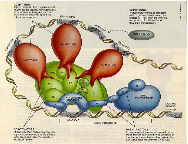
(13) reverse transcript to cDNA (complementary DNA) for RNA amplification.. Figure 1.1 Central dogma of molecular biology. (The figure is obtained from http://cats.med.uvm.edu/.../1_centraldogma_wisc_13.jpg). 1.1.2 Transcriptional Start sites (TSS) Transcription, the process whereby RNA copies are made from sections of the DNA genome, is directed by promoter regions (Down and Hubbard 2002). The promoter is a DNA sequence which is usually located on the upstream of a gene transcriptional starting site (TSS). The core promoter, a region of about 100 base-pairs flanking the transcriptional start site (TSS), serves as the recognition site for the basal transcription apparatus (Ohler, Liao et al. 2002). Figure 1.2 shows a simplified gene structure and promoter region. When RNA polymerase II and some kinds of transcription factors bind onto the gene promoter region 2.

(14) together, the transcription of a gene will be activated and the messenger RNA (mRNA) will be transcribed from the DNA sequence. We have known that the promoter region is always located on the upstream of a gene and we will try to find out some hallmarks nearby the known transcriptional start sites. Thus, we can identify the transcriptional start sites on the unknown DNA sequences by using these hallmarks.. Figure 1.2 A simplified gene structure.. 1.1.3 Transcriptional Regulation Transcriptional regulation is one of the most important means of gene regulation. Uncovering transcriptional regulatory networks helps us to understanding the complex cellular process (Xing and van der Laan 2005). As. 3.

(15) shown in the Figure 1.3, gene transcription is regulated by transcription factors (TFs) which are binding mostly and specifically to the 5’ end of genes. The RNA polymerase II promoter is the critical region that regulates differential transcription of protein coding genes (Solovyev and Shahmuradov 2003), and is located near the transcription start site (TSS). A typical promoter region is believed to comprise short DNA sequences known as regulatory elements, which includes transcription factor binding sites (TFBSs) (Prakash and Tompa 2005). About 10~15% of mammalian DNA re-associated very rapidly. This class includes tandem repeats. It includes Satellites (100 kb to over 1Mb), Ministatellites (1kb ~ 20kb), Microsatellites (Short Tandem repeats, 1~ 6 base in a region less than 150 base). Interspersed repeats are repeated DNA sequences located at dispersed regions in a genome. They are also known as mobile elements or transposable elements. In mammals, the most common mobile elements are LINEs (Long Interspersed Nuclear Elements) and SINEs (Short Interspersed nuclear Elements). The structure of eukaryotic promoters is more complex than prokayotic promoters and they have several sequence motifs, for example TATA box, CCAAT box, GC box, and INR box (Kanhere and Bansal 2005). Therefore, some concepts are also used to analyze the promoter, including the presence of CpG islands close to the transcription start site, the presence of a specific 4.

(16) transcription factor binding site, statistical properties of proximal and core promoters rather than other genomic sequences, the orthologous gene promoters, and restricting the promoter region from using information from mRNA transcripts (Bajic, Tan et al. 2004).. Figure 1.3 Transcriptional regulation. (The figure is obtained from http://www.wellesley.edu/.../06eukaryotes.jpg). 1.2 Motivation To accurately determine the core promoter in gene upstream is the first step to decipher the regulation of gene transcription. In recent years, powerful 5.

(17) computational techniques have increasingly been used to analyze annotated DNA sequences to uncover the secret of human genomes. Gene promoter prediction is important for guiding experimental biologists to find novel gene promoter region. However, the existing promoter prediction tools result in low sensitivity or low specificity. The low prediction accuracy stems from the low quality of regulatory features or training data source. Therefore, a computational method integrated with good regulatory features should be proposed.. 1.3 Goal Developing an efficient and effective system to identify gene transcriptional start sites is important in silico tools for guiding experimental biologists. However, the existing promoter prediction programs can only be used for minor reference because of them results in low sensitivity or low specificity. Therefore, the main purpose of this study is to incorporate the powerful computational method with useful regulatory features of core promoters for gene promoter identification that results in high prediction sensitivity and specificity. This study can help researchers identifying gene transcriptional promoter region more efficiently and exactly.. 1.4 Challenges Before extracting the useful regulatory features for core promoters, the 6.

(18) experimentally verified transcriptional start sites need to be obtained. In this thesis, the main source of the known transcriptional start sites were obtained from DBTSS and the genomic sequences of the mammalian genomes were obtained from NCBI build 35. All the promoter sequences obtained from DBTSS were stored into our databank for analyzing the core promoter region. However, the length of sequences obtained from DBTSS was 1201 bps (from -1000 to +200), which was too short to completely analyze the flanking region of TSS. We used the Blast program to align the promoter sequence of DBTSS to the genomic sequences of NCBI build 35, then the longer sequences of 6001 (from -3000 to +3000) were obtained. Besides, the problem of identifying gene transcriptional start sites itself remains some difficult challenges. The most important one challenge is that no reliable dataset of experimentally verified transcriptional start sites can be used to analyze the specifically regulatory elements of promoter. Moreover, the existing promoter prediction tools result in low numbers of true positive predictions and high numbers of false positive predictions. The detailed description of the existing promoter prediction methods will be discussed in chapter 2. The research scope of this thesis is concentrated on mammalian (human and mouse) genomes. The reason for using the mammalian genomes is that the sequences of gene transcriptional start sites obtained from DBTSS just had human and mouse. In addition, the reason for obtaining the sequences of gene 7.

(19) transcriptional start sites from DBTSS is its amount much more than other databases. Therefore, we constrict our scope to identify transcriptional start sites in mammalian genomes.. 8.

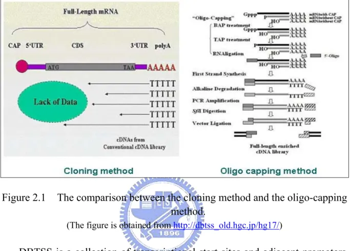
(20) Chapter 2 Related Works 2.1 Experimental TSS data source Two popular experimentally verified transcriptional start site databases, such as Eukaryotic Promoter Database (EPD) and Database of Transcriptional Start Site (DBTSS), were widely used to analyze the promoter region.. 2.1.1 Eukaryotic Promoter Database (EPD) The Eukaryotic Promoter Database (EPD) is an annotated non-redundant collection of eukaryotic POL II promoters, for which the transcription start site has been determined experimentally (Schmid, Praz et al. 2004). EPD is a collection of 4,810 eukaryotic POL II promoters. Tools for analysing sequence motifs around TSSs defined in EPD are provided by the signal search analysis server. EPD can be accessed at http://www.epd. isb-sib.ch.. 2.1.2 Database of Transcriptional Start Sites (DBTSS) Suzuki et al developed a novel method namely oligo-capping to collect the full-length cDNA libraries. The different between cloning method and oligo-capping method is shown in Fig. 2.1. The characteristics of oligo-capping method are extensive, high throughput, and high accuracy. DBTSS (Suzuki, Yamashita et al. 2004) was constructed in 2002 based on the full-length cDNA 9.

(21) libraries.. Figure 2.1. The comparison between the cloning method and the oligo-capping method. (The figure is obtained from http://dbtss_old.hgc.jp/hg17/). DBTSS is a collection of transcriptional start sites and adjacent promoters, which are experimentally determined by intensive analyses of full-length cDNAs. In order to extract biological insight from the compiled sequence information, search engines for putative transcription factor binding sites are implemented. Also, for molecular evolutionary studies of the transcriptional regulations, detailed sequence alignments of the promoters between human, mouse and other model organisms are provided. DBTSS is available on the web in Japan at http://dbtss.hgc.jp. The positional information of the TSSs, sequences of the promoters and related information can also be downloaded in flat file form from the download site. The current release of DBTSS (5.1) contains TSS 10.

(22) information of 15,262 and 14,162 genes determined by 1.4 and 0.4 million cDNAs in humans and mice respectively.. 2.2 Related Works of Gene Promoter Prediction Tools Gene promoter prediction is important in silico analysis for guiding experimental biologists. Although several gene promoter prediction tools had been developed, wet-lab biologists didn’t much believe that because of the low prediction accuracy. Until the appearance of PromoterInspector (Scherf, Klingenhoff et al. 2000), gene promoter prediction tools suffered from low accuracy. After the appearance of PromoterInspector, several efficient gene promoter prediction tools have also been developed. In the following, we expand further on their reviews and include more recent research on gene promoter prediction.. 2.2.1 NNPP (Version 2.2) NNPP 2.2 (Reese 2001) is constructed of time-delay neural networks. The network model is a special case of a feed-forward neural network, which has been successfully applied to voice recognition. Time-delay neural networks slightly differ from feed-forward neural networks in the design of the hidden layer. The hidden nodes of a standard feed-forward model are determined by experiment or by lemma. In a time-delay model, the hidden nodes are. 11.

(23) determined by the number of the input nodes and the input size of the receptive fields. Therefore, the input layer and the hidden layer are no longer fully connected. The hidden nodes in a hidden layer are only connected to input nodes within a particular receptive field. In a time-delay model, the hidden node is also called a feature node and is known as weight sharing in neural network technology. In the training process, all the weights in the same receptive filed will be calculated and then copied to each other. However, the weights computed between the hidden nodes and the output nodes are still based on standard feed-forward algorithms. To optimize promoter prediction accuracy, two time-delay neural network models which recognize TATA-box with 30 bp (-40 bp to -10 bp from the TSS) and Inr (-14 bp to +11 bp from the TSS) regions of promoters are used. A combined model with 51 bps (-40 bps upstream to +11 bps downstream of TSS) is used along with the two models mentioned above for promoter prediction. The testing results showed that NNPP demonstrated 75% true positives for a fruit fly genome with a length of 2.9 Mbps.. 2.2.2 McPromoter MCPromoter (Ohler, Stemmer et al. 2000) coordinated three interpolated Markov chains (IMCs) to look for eukaryotic polymerase II TSSs in genomic DNA. It consists of a model for promoter sequences and a mixture model for non-promoter sequences, containing sub-models for coding and non-coding 12.

(24) sequences. To localize TSSs, a window of 300 bases is shifted over the sequence in steps of 10 bases. At every position, the difference between the log likelihood of the promoter and the non-promoter model is computed. The resulting plot describes the regulatory potential over the sequence and is smoothed by a median and hysteresis filter (see Duda and Hart 1973) to eliminate single false predictions and reduce the high number of neighboring minima that are due to noise. The program then makes a prediction for each local minimum below a pre-specified threshold. The training dataset are extracted from the EPD which contains a total of 565 vertebrate promoter sequences, and each contained 250 bp upstream and 50 bp downstream from the TSS. After the five-fold cross validation evaluation, the system reached an 84% correlation coefficient for promoters versus coding regions and achieved a 53% correlation coefficient for promoters versus non-coding regions.. 2.2.3 Eponine Eponine (Down and Hubbard 2002) proposed a probabilistic method for detecting transcription start sites (TSS) in mammalian genomic sequence, with good specificity and excellent positional accuracy. Eponine models consist of a set of DNA weight matrices recognizing specific sequence motifs. Each of these is associated with a position distribution relative to the transcription start site. 13.

(25) Eponine has been tested by comparing the output with annotated mRNAs from human chromosome 22. From this work, they estimate that using the default threshold (0.999), it detects >50% of transcription start sites with 70% specificity. However, it does not always predict the direction of transcription correctly. It’s an effect which seems to be common among computational TSS finders.. 2.2.4 CpGProD CpGProD (Ponger and Mouchiroud 2002) is a program dedicated to the prediction of promoters associated with CpG Islands in mammalian genomic sequences. In vertebrate genomes, the CpG Islands (CGIs) are involved in DNA methylation of gene transcription. 50-60% of the human genes exhibit a CGI over the transcription start site (TSS) but not all the CGIs are associated with promoter regions (Larsen, Gundersen et al. 1992). CpGProD uses a CGI definition more stringent than that proposed by Gardiner-Garden and Frommer (1987). CpG Island are defined as DNA regions longer than 500 nucleotides (instead 200 bp), with a moving average G + C frequency above 0.5 and a moving average CpG observed/expected (CpG o/e) ratio greater than 0.6. Although it is strictly dedicated to this particular promoter class corresponding to ≈50% of the genes, CpGProD exhibits a higher sensitivity and specificity than other tools used for promoter prediction.. 14.

(26) 2.2.5 PromoterInspector PromoterInspector (Scherf, Klingenhoff et al. 2000) is one of the most well-known content-based gene TSSs prediction tools, which gives attention to analyzing genetic context instead of context location. Its main idea is to extract common sequence features from sequences and generate a set of context features called IUPAC (International Union of Pure and Applied Chemistry) word dictionaries. IUPAC word dictionaries are composed of an IUPAC group which is defined by a set of oligonucleotides and a number of undefined base pairs (i.e. the letter “N” could represent A, C, G or T). To optimally distinguish a promoter region from an un-annotated DNA sequence, PromoterInspector introduces not only a promoter region as the training set but also three non-promoter sequences, that is, exon, intron, and 3’UTR. These training data sets then generate three classifiers: promoter and exon, promoter and intron, and promoter and 3’UTR. These three classifiers are the basis of PromoterInspector. In the experiment results, the vertebrate promoter training data were extracted from EPD, and the non-promoter exon and intron were randomly downloaded from NCBI GenBank; the 3’UTR was selected from the UTR database. The valuation data that were collected by Ficktt and Hatzigeorgiou were tested. The greatest advantage of PromoterInspector seems to be that of dramatically reducing the false positives. This advantage can help lab researchers avoid. 15.

(27) unnecessary experiments or help other prediction tools further and exactly locate the transcriptional start sites.. 2.2.6 Promoter 2.0 Promoter 2.0 (Knudsen 1999) combines several neural networks. Each neural network model uses perceptron-like algorithms. In the training phase, the inputs of the neural networks are a small window of DNA sequence and the output of other networks. For example, giving a network with a given input window size and a set of weights, the network scans along a DNA sequence and records the scores that are generated from every segment. Next, another new network with the same structure but with different weight scans the same DNA sequence. The highest score of each of all the previous networks for the same DNA sequence will be multiplied by a separation function. The result will become the input of this new network. In Promoter 2.0, there are four networks responded to TATA-box, cap site, CCAAT-box and GC box. To optimize these neural networks, genetic algorithms are used to randomly choose and change an individual weight. If the performance of network improved, the new weight was kept. The new weight was ignored if the performance did not improve. Nevertheless, the crossover operation of genetic algorithms is not used in Promoter 2.0. The training and testing data of Promoter 2.0 were 100 vertebrate sequences. For a positive set, 200 bps upstream of the cap site was selected as the promoter sequence. In contrast, 200 bps downstream of the cap site was 16.

(28) assigned as the non-promoter sequence; Promoter 2.0 reported 63% true positives for its testing data.. 2.2.7 Dragon Promoter Finder The Dragon Promoter Finder 1.2 (DPF) (Bajic, Seah et al. 2002) is an gene promoter prediction model for vertebrates. The DPF consists of a nonlinear promoter recognition model, sensors for recognizing specific functional regions of DNA, signal processing, and artificial neural networks. Before using the DPF, a user has to supply a DNA sequence and a selected accuracy range to the DPF system. The DPF then reads the DNA sequence by a sliding window and shifts one base pair each time. The data window’s content passes through three sensors. Each sensor responds to a specific functional region, such as a promoter, exon and intron. A non-linear signal processing model further analyzes the sensor’s output and feeds it into to a neural network to ascertain the input DNA sequence and determine if a promoter region exists. The DPF 1.3 extends the capability for recognizing a GC-rich or GC-poor DNA sequence. The DPF used 793 different vertebrate promoter sequences from EPD as positive training set; each sequence was 250 bps long, covering 200 bps upstream and 50 bps downstream from the TSS. For a negative training set, the DPF used 800 coding-exon and 4000 intron sequences. To further tune the system parameters, DPF extended 400 3’ UTR human sequences and 200 human exon and 500 human intron sequences to the training set. Each sequence 17.

(29) was also 250 bps long. The final testing data contained 146 human and humanviral sequences, which contained 159 TSSs. The DPF showed 66% true positives, which outperformed other tools significantly.. 2.2.8 Dragon Gene Start Finder Dragon Gene Start Finder (Dragon GSF) (Bajic and Seah 2003) combines three systems. The first one is Dragon Promoter Finder (DPF) (Bajic et al (2003), the second one is the system which estimates the presence of the CpG Islands, and the third one combines information from these two into the final predictions. The third system performs the sensor fusion function utilizing data preprocessing and an artificial neural network (ANN). The combination algorithm will only select the one of possibly many predicted TSS locations in the region [-3700,+3700] relative to the central point of the CpG Island, such that jointly with the other input data the ANN produces the highest score above the selected threshold. Dragon GSF made every effort not to mislead the user with claims of superior performance. Dragon GSF presented the performance as found on the tests on different genomic sequences including whole human chromosomes 4, 21, and 22. Based on these results Dragon GSF infer that the gene start finding capabilities of Dragon GSF system are among the best currently available. The estimated performance for the human genome of Dragon GSF implies sensitivity of ~65% (relative to all promoters), sensitivity of ~88% relative to the CpG 18.

(30) Island related promoters, and positive predictive value of ~78% relative to all known genes.. 2.2.9 First Exon Finder First Exon Finder (FirstEF) (Davuluri, Grosse et al. 2001) uses different discriminating functions structured as a decision tree to predict the first exons and promoters in a gene. The probabilistic models are designed to find potential first donor sites and CpG-related and non-CpG-related promoter regions based on discriminating analysis. For each potential first donor and upstream promoter region, FirstEF decides whether the intermediate region could be a potential first exon based on a set of quadratic discriminating functions. Test and training sets came from the same database. FirstEF’s accuracy was tested by ten-fold cross-validation analysis and running the program on the complete exon sequences of genes in chromosomes 21 and 22. First exons predictions were considered true positives if the predicted first donor site was identical to the real donor site and the predicted transcriptional start site (TSS) fell within the region between 500 bp before and 200 bp after the real TSS. Recall, precision, and the correlation coefficient were used to judge the accuracy of FirstEF.. 2.2.10 Summary of Gene Promoter Prediction Tools. 19.

(31) The gene promoter prediction tools introduced in this Session are summarized in Table 2.1. No previously developed tools can achieve the performance with higher sensitivity than 70% and higher specificity than 70%.. 20.

(32) Table 2.1 Tool. Method. Species. Summary of gene promoter prediction tools.. Feature Consider. Data Source. Citation. Sn.. Sp.. False positive rate. Acc.. Available. 53.5%. 73.5%. -. -. Yes. 68%. -. 8%. -. No. 70%. -. 7.2%. -. Yes. 56%. 39%. -. -. Yes. 48%. 85%. -. -. No. Eponine. Relevance Vector Machine (RVM). Mammalian. TATA box in a G+C rich domain. EPD. Reese 2001. Promoter 2.0. ANN. Vertebrate. Four TFBSs (TATA box, CCAAT box, GC box, Inr). EPD. Ohler, Stemmer et al. 2000. NNPP 2.2. ANN. Drosophila. TATA box & Inr. EPD. CpGProD. Statistics based. mammalian. CpG Island. GenBank. Vertebrate. IUPAC. EPD. CpG Island related. EPD. Knudsen 1999. 60.17%. -. -. -. No. DBTSS. Bajic, Seah et al. 2002. 65.10%. -. -. 77.80%. No. EPD. Bajic and Seah 2003. 52.1%. 40.3%. -. -. Yes. NCBI. Davuluri, Grosse et al. 2001. 79.3%. 53.5%. -. -. No. PromoterInspector Statistics based. Human Chr. 22 Human Chr. 4,21,22. Dragon PF. ANN. Dragon GSF. ANN. McPromoter. ANN. Human Chr. 22. First Exon Finder. Quadratic discriminating analysis. Human Chr. 21,22. G+C rich &G+C poor Interpolated Markov Model CpG Island related. * Sn. = Sensitivity, Sp. = Specificity, Acc. = Accuracy.. 21. Down and Hubbard 2002 Ponger and Mouchiroud 2002 Scherf, Klingenhoff et al. 2000.

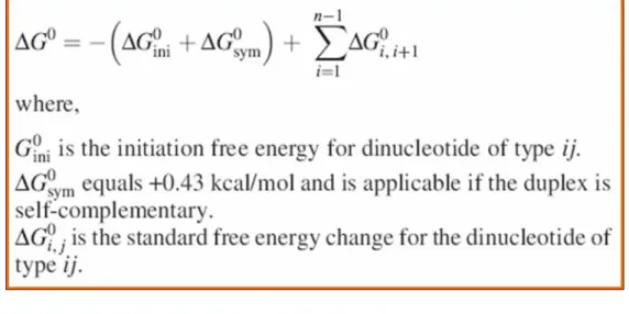
(33) 2.3 DNA stability Aditi Kanhere et al. (Kanhere and Bansal 2005) devised a novel regulatory feature, DNA stability, for prokaryotic promoter prediction. The DNA stability is the structural property of the fragment of the DNA duplex, which is calculated based on the minimum free energy created by the hydrogen bond of the A-T and C-G pairs. There are several factors that stabilize a DNA double helix. Among the significant factors are: 1. Stacking Interaction 2. Watson-Crick Hydrogen Bonding Interaction 3. Interaction with Water Molecules and Metal Ions SantaLucia et al. (SantaLucia 1998) use the unified standard free energy of ten dinucleotides duplexes, such as AA/TT, AT/TA, TA/AT, CA/GT, GT/CA, CT/GA, GA/CT, CG/GC, GC/CG, and GG/CC (SantaLucia 1998), to calculate the standard free energy change of a DNA oligonucleotide based on dinucleotid e composition. The free energy formula and the calculation example that used by Santalucia were shown in Fig. 2.2 and Fig. 2.3, respectively.. 22.

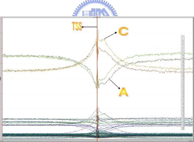
(34) Figure 2.2. The formula of calculating the free energy for the DNA sequence.. Figure 2.3. The example of free energy computation.. Aditi Kanhere and Manju Bansal presented a novel prokaryotic promoter prediction method based on DNA stability (Kanhere and Bansal 2005). They showed that the promoter region is less stable and hence more prone to melting as compared to other genomic regions. Figure 2.4 shows the distributions of average free energy of DNA duplex formation, and reveals a peak near the TSS, lying 23.

(35) between -10 and -30 region, which corresponds to the TATA box in the eukaryotic promoter sequences.. Their analysis also showed that a method of promoter. prediction based on the differences in the stability of DNA sequences in the promoter and non-promoter region works much better compared to existing prokaryotic promoter prediction programs, which are based on sequence motif searches. At present the method works optimally for genomes such as that of Escherichia coli, which have near 50 % G+C composition and also performs satisfactorily in case of other prokaryotic promoters.. Figure 2.4. Average free energy nearby TSSs of three species.. 2.4 Support Vector Machine (SVM) Support Vector Machine (SVM) is a popular technique for classification (Hsu, Chang et al.). A support vector machine (SVM) is a supervised learning technique from the field of machine learning applicable to both classification and regression. 24.

(36) Rooted in the Statistical Learning Theory developed by Vladimir Vapnik and co-workers at AT&T Bell Laboratories in 1995(Vapnik 1995), SVMs are based on the principle of Structural Risk Minimization. As shown in Fig. 2.5, the goal of SVM is to produce a model which predicts target value of data instances in the testing set which are given only the attributes.. Figure 2.5. The concept of SVM. LIBSVM (Chang and Lin 2001) was developed by Chih-Chung Chang and Chih-Jen Lin. LIBSVM is an integrated software for support vector classification, regression, and distribution estimation. LIBSVM supports the multi-class classification. Since version 2.8, it implements an SMO-type algorithm. Their goal is to help users from other fields to easily use SVM as a tool. The SVM process 25.

(37) overview is shown in Fig. 2.6.. Figure 2.6. SVM process overview. 26.

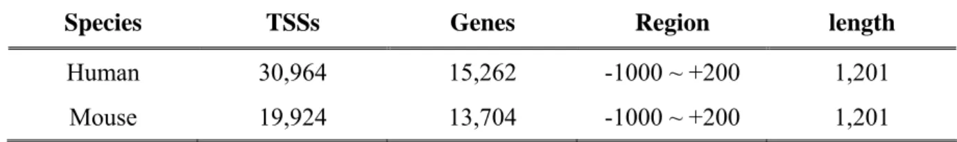
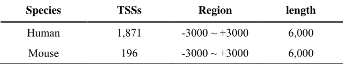
(38) Chapter 3 Material and Methods 3.1 Materials The experimentally verified transcriptional start sites of DBTSS and human genome sequence of NCBI are used in this research.. 3.1.1 Database of Transcriptional Start Site (DBTSS) and EPD We extract the flanking sequence of experimentally verified transcriptional start sites form DBTSS. The vision of DBTSS we used is release 5.1.0. As given in Table 3.1, it contains 30,964 human promoter sequences which are length 1,201 base pairs (from -1,000 to +200) within 15,262 genes. And 8,308 human genes are found to have putative multiple promoters. As shown in Table 3.2, 1,871 human promoter sequences with length 6,000 base pairs (from -3000 to +3000) were obtained from EPD for the independent test, as well as the 196 mouse promoter sequences.. Table 3.1 The statistics of human and mouse experimentally TSSs in DBTSS. Species. TSSs. Genes. Region. length. Human. 30,964. 15,262. -1000 ~ +200. 1,201. Mouse. 19,924. 13,704. -1000 ~ +200. 1,201. 27.

(39) Table 3.2 The statistics of human and mouse experimentally TSSs in EPD. Species. TSSs. Region. length. Human. 1,871. -3000 ~ +3000. 6,000. Mouse. 196. -3000 ~ +3000. 6,000. 3.1.2 NCBI Genome Sequences We extract the human whole genome sequences from NCBI. The vision we used is NCBI build 35 release 1. The total length of sequences assembled was 3,021,400,000 base pair.. 3.2 Methods We developed a gene promoter prediction method which integrates novel regulatory features with Support Vector Machine (SVM). Figure 3.1 shows the system flow in this works, there are three stages in developing TSSs prediction method. Stage 1 is to construct the training dataset for the TSS prediction. In the Stage 2, three kinds of regulatory features in the flanking region of experimentally verified TSSs are extracted and analyzed. Finally, Stage 3 uses the SVM to construct the classifying model for the three selected features and evaluate the prediction performance. We will discuss every stage in detailed as following.. 28.

(40) Figure 3.1. System flow of prediction tool developing.. 3.2.1 Dataset Construction The experimentally verified human promoter sequences were extract from DBTSS which contains 30,964 experimentally TSSs. All the promoter sequence 29.

(41) length of DBTSS are 1,201 base pairs (bps), which is extracted from 1,000 bps upstream to 201 bps downstream of the TSS. Because of the sequences we obtained from DBTSS were too short to be analyzed, we use BLAST to align the promoter sequences of DBTSS to the human whole genome sequence. With the alignment preprocess, we got the 6,000 bps sequence length of each promoter sequence (from 3,000 bps upstream to 3000 downstream of the TSS). After the alignment preprocessing, we should make sure that each promoter sequence only contains just one TSS in the region of 6,000 bps sequence length. Therefore, we dropped the promoter sequences that had multiple experimental TSSs in the region of 6,000 bps sequence length. Finally, it remains 6,464 promoter sequences which have unique TSS in the region of 6,000 bps sequence length. Furthermore, we also consider if the sequences in our dataset contains CpG Island or not. We used the CpG island prediction tool “CpGproD” to classify all the 6,464 promoter sequences into two groups (has CpG Isalnd or not). Table 3.2 shows the number of sequences of three groups, Group 1: all promoter sequences; Group 2: promoter sequences without CpG Island; Group 3: promoter sequences with CpG Island. Table 3.3 Numbers of sequence of group 1, 2, and 3. Group 1 (All) 2 (Non-CpG) 3 (CpG). Numbers of sequence 6,464 1,566 4,898 30.

(42) 3.2.2 Feature Extraction In the feature extraction stage, we were trying to extract the useful regulatory features of promoter sequences to accurately identify human TSSs. We surveyed many related promoter prediction methods, and finally extracted three classifying features such as statistically significant 6-mer pattern, nucleotide composition, and DNA stability.. 3.2.2.1 Statistically Significant 6-mer Pattern First of all, we must to define the positive set and negative set of training data. Positive set was extracted from flanking regions of TSSs liked the upstream 200 to downstream 100 of TSS. The whole genomic regions other than the regions of positive set were defined as negative set. Following, we computed occurrence probability of 6-mer patterns for positive set and negative set according to the formula: n. P=. ∑S. (1). i =1. n. ∑ Len − 5 i =1. , where P denotes the occurrence probability, S denotes the number of 6-mer pattern occurrence in one sequence, and Len denotes the length of a sequence. After that we computed the occurrence ratio of every 6-mer pattern. The formula of Occurrence ratio: 31.

(43) O=. Ppos Pneg. (2). , where O denotes occurrence ratio, Ppos denotes the probability of positive set, and Pneg denotes the probability of negative set. Finally, by optimized the top occurrence ratio pattern number, we chose top 60 occurrence rate of these patterns as features.. 3.2.2.2 Nucleotide Composition We try to analyze the nucleotide composition in the promoter region, the average occurrence rate of monomer, dimer, and trimer nucleotide are calculated in window size 20 bps sliding on the promoter sequence. The formula of average nucleotide occurrence rate: N. AVG =. ∑P. (3). i =1. N. , where AVG denotes average nucleotide occurrence rate of the sliding window with size 10 bps, P denotes pattern occurrence times of every sequence, and N denotes the total number of sequences in our dataset. Then we specify the monomer nucleotide A and C occurrence rate as standard and computed a Pearson correlation coefficient for the other patterns with these two patterns to determine whether their correlation coefficient values are highly correlated. The cutoff value of the Pearson correlation coefficient is set to 0.8 to decide whether two patterns highly correlated or not. 32.

(44) 3.2.2.3 DNA Stability We computed the average of free energy of the 15 bps nucleotides and shift in the size of 5 bps nucleotides in our dataset sequences. The formula of DNA sequences of free energy is shown in Figure 3.2. The standard free energy change ( ΔG370 ) corresponding to the melting transition of an ‘n’ nucleotide (or ‘n-1’ dinucleotides) long DNA molecule, from double strand to single strand, is calculated as shown in Fig. 3.2 (Kanhere and Bansal 2005). ΔGini0 denotes two types of initiation free energy : “initiation with terminal G⋅C” and “initiation with 0 terminal A⋅T”; ΔGsym is +0.43 kcal/mol and is applicable if the duplex is. self-complementary, and ΔGi0, j represents the standard free energy change for type ij dinucleotide. In the present calculation, each promoter sequence is divided into overlapping windows of 15 bps (or 14 dinucleotide steps), and for each window the free energy is calculated as shown above. We used the free energy of the 15 bps nucleotides and shift in the size of 5 bps nucleotides as features.. 33.

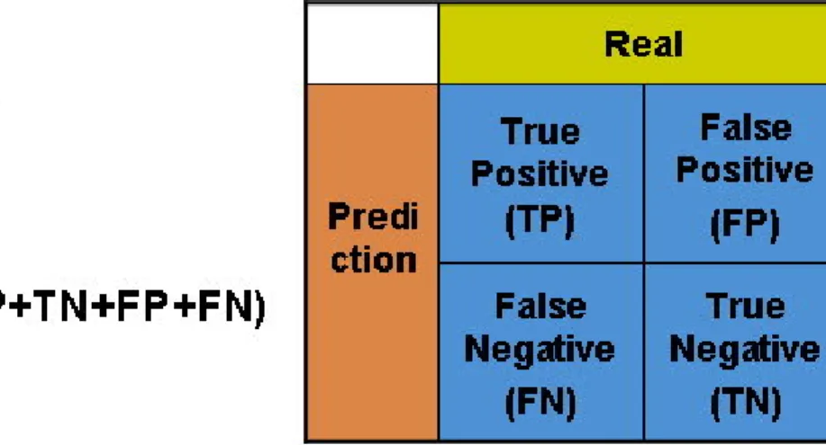
(45) Figure 3.2. Formula of DNA sequences free energy.. Aditi Kanhere et al. (Kanhere and Bansal 2005) demonstrated that the change in DNA stability appears to provide a much better clue than the usual sequence motifs. Therefore, this work provides the DNA stability of the promoter region to enhance the promoter identification.. 3.2.3 Model Learning and Evaluation After the process of feature extraction, the three kinds of feature are trained by LIBSVM (Chang and Lin 2001) which developed by Chih-Chung Chang and Chih-Jen Lin. LIBSVM is an integrated software for support vector classification, regression, and distribution estimation. The three features of the positive and negative training set are transformed into LIBSVM input format, and the input values are normalized before the SVM model construction. The constructed SVM models of the three kinds of feature are evaluated by K-fold cross-validation. We used 5-fold cross validation to evaluate the prediction performance of the SVM-trained model. To express the prediction quality of the models, we applied 34.

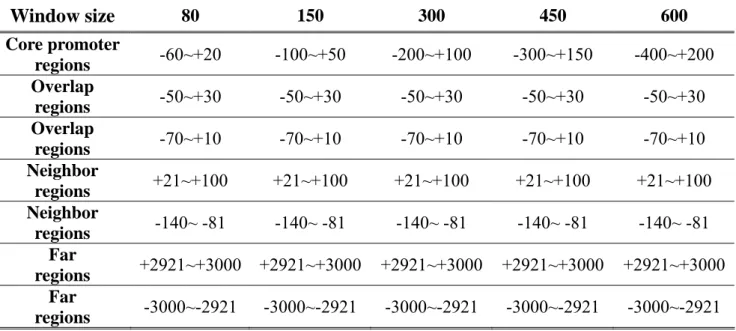
(46) several criteria. These evaluation criteria included sensitivity, specificity, accuracy, and precision. Figure 3.3 shows the definition of sensitivity, specificity, accuracy, and precision. To optimize our models’ performance, we do parameter optimization in the window size, selected numbers of 6-mer pattern, and feature combinations.. Figure 3.3. The definition of four performance measures.. To fairly evaluate the prediction performance of the gene promoter prediction method, an evaluation benchmark should be constructed. By surveying previous related works, one of the several evaluation benchmarks they used was chosen by us. As shown in Fig. 3.4, the positive sets were extracted from the positive region, and negative sets were randomly extracted from the six kinds of negative regions. There are five kinds of window sizes for positive set including 80, 150, 300, 450, and 600 bps. We show the regions of positive and six kinds of negative in detail in Table 3.3. 35.

(47) Figure 3.4. Evaluation Benchmark.. Table 3.4 Positive region and six kinds of negative region of window size we optimized. Window size. 80. 150. 300. 450. 600. Core promoter regions Overlap regions Overlap regions Neighbor regions Neighbor regions Far regions Far regions. -60~+20. -100~+50. -200~+100. -300~+150. -400~+200. -50~+30. -50~+30. -50~+30. -50~+30. -50~+30. -70~+10. -70~+10. -70~+10. -70~+10. -70~+10. +21~+100. +21~+100. +21~+100. +21~+100. +21~+100. -140~ -81. -140~ -81. -140~ -81. -140~ -81. -140~ -81. +2921~+3000. +2921~+3000. +2921~+3000. +2921~+3000. +2921~+3000. -3000~-2921. -3000~-2921. -3000~-2921. -3000~-2921. -3000~-2921. 36.

(48) Chapter 4 Results Here we present the results of our evaluation benchmark to show the prediction performance of the constructed models based on Support Vector Machine (SVM). We also compared our models’ accuracy with several existing gene promoter prediction tools that we obtained.. 4.1 Feature Observations Three features such as statistically significant 6-mer patterns, nucleotide composition, and DNA stability of promoter sequences are extracted and observed to decide some parameters such as the number of 6-mer patterns and the window size of positive set.. 4.1.1 Statistically Significant 6-mer Patterns By optimizing the selected numbers of pattern, we selected the top 60 patterns as our prediction feature .The selected top 60 patterns of group 1 are given in Table 4.1. The selected top 60 patterns of group 2 are given in Table 4.2. The top 60 selected patterns of group 3 are given in Table 4.3. We will show top 100 patterns in detail in appendix.. Table 4.1 Top 60 selected pattern of group 1 (all). 37.

(49) CGCGCG GCGCGC CGCCGC GCGGCG CGGCGC GCGCCG CGCGGC GCCGCG CCGCCG CGGCGG CCGGCG CGCCGG AGCGCG CGCGCT CCGCGG. Table 4.2 CGCGAA CCGCCC ATCCGG CTGCGG CTTCCG TCGACG CGGCAG CGCGGA CGGCGA GCGGCA TCCGCA GCCGGA AGGGCG ACCGGA GGCCGT. Table 4.3 CGCGCG CGGCGC CCGCCG AGCGCG TGCGCG CTCGCG CGCGAC CCGCGC CGGCGA CGCGTC CCGCGA CGACCG GGGGCG. CGCGCA TGCGCG CCCGCG CGCGGG CGCGAG CTCGCG CGCGGA TCCGCG TCGCGA CGCGAC GTCGCG CGTCGC GCGACG CCGCGC GCGCGG. CGCCGA TCGGCG CGGCGA TCGCCG CGAGCG CGCTCG CCGCGA TCGCGG CGCGTC GACGCG ACGCGC GCGCGT CGACGC GCGTCG CGACCG. CGGTCG CGGCCG CGCCCC GGGGCG ACGCCG CGGCGT GCCGCC GGCGGC CCCCGC GCGGGG CCGCCC GGGCGG GCGGCC GGCCGC CCGTCG. Top 60 selected pattern of group 2 (non-CpG island). TTCGCG GGGCGG CCGGAT CGCGAG ACGTCA CCGGAA CTGCCG TCCGCG TCGCCG TGCCGC TGCGGA TCCGGC CGCCCT TCCGGT GCCGAC. CGCCCC CCCCGC GACGTC CTCGCG TGACGT TTCCGG ACTCGC CCGCGA CGACTC CGGCCC CGGGGC GCCCGA CGTCAC GGGCCC GTCGGC. GGGGCG GCGGGG CCGCAG CGGAAG CGTCGA GCCGGC GCGAGT TCGCGG GAGTCG GGGCCG GCCCCG TCGGGC GTGACG ACGGCC CGGCAC. Top 60 selected pattern of sequences group 3 (CpG island). GCGCGC GCGCCG CGGCGG CGCGCT CCCGCG CGCGGA GTCGCG GCGCGG TCGCCG GACGCG TCGCGG CGGTCG ACGCCG. CGCCGC CGCGGC CCGGCG CCGCGG CGCGGG TCCGCG CGTCGC CGCCGA CGAGCG ACGCGC CGACGC CGGCCG CGGCGT 38. GCGGCG GCCGCG CGCCGG CGCGCA CGCGAG TCGCGA GCGACG TCGGCG CGCTCG GCGCGT GCGTCG CGCCCC GCCGCC.

(50) GGCGGC GCGGGG. GCGGCC CCGTCG. GGCCGC CGACGG. CCCCGC CCGCCC. 4.1.2 Nucleotide Composition The distributions of monomer, dimer, and trimer nucleotide composition of group 1, 2, and 3 are shown in Fig. 4.1, 4.2, and 4.3, respectively. The cutoff value of the Pearson correlation coefficient is set to 0.8 to decide whether two distribution patterns highly correlated or not. The selected highly correlated patterns of monomer, dimer, and trimer nucleotide composition are given in Table 4.4, 4.5, and 4.6, respectively.. Figure 4.1. The distribution of monomer, dimer, and trimer nucleotide composition of group 1 (all).. 39.

(51) Table 4.4 The selected highly correlated patterns of nucleotide composition of group 1 (all). C.C. with A >0.8. C.C. with C >0.8. No select. Monomer and Dimer. T,AA,AT, AC,TA,TT,CA. G,CC,CG, GC,GG. AG,TC,TG, CT,GA,GT. Trimer. A A A , A AT, A A C A A G, ATA , AT C AT T, AT G, A C A A C T , A G ATA A TA C , TAT, TA G T TA , T T T, T C A T G A , C A A , C AT CTA. ACG,AGC,TCC,TCG CTC,CCC,CCG,CGA CGT,CGC,CGG,GAC GTC,GCC,GCG,GGA GGC,GGG. ACC,AGT,AGG,TTC TTG,TCT,TGT,TGC TGG,CAC,CAG,CTT CTG,CCA,CCT,GAA GAT,GAC,GAG,GTT GTG,GCA,GCT,GGT. Figure 4.2. The distribution of monomer, dimer, and trimer nucleotide composition of group 2 (non-CpG island). 40.

(52) Table 4.5. Monomer and Dimer. Trimer. The selected highly correlated patterns of nucleotide composition of group 2 (non-CpG island). C.C. with A >0.8. C.C. with C >0.8. No select. AA,AT,TA. G,AG,CC,CG,CT GC,GG,TC. T,AC,CA,GA,GT,TG,TT. ACG,AGC,AGG,CAG C C A , C C C , C C G, C C T CGA,CGT,CGC,CGG CTC,CTG,GAC,GAG GCC,GCG,GCT,GGA GGC,GGG,GTC,TCC TGC,TGG. AAC,AAG,AAT,ACA ACC,ACT,AGA,AGT AT C , AT G, AT T, C A A C A C , C AT, C TA , C T T GAA,GAT,GCA,GGT G TA , G T G, G T T, TA A TA C , TA G, TAT, T C A T C T, T G A , T G T, T TA TTC,TTG,TTT. AAA,ATA. Figure 4.3. The distribution of monomer, dimer, and trimer nucleotide composition of group 3 (CpG island).. 41.

(53) Table 4.6. Monomer to Dimer. Trimer. The selected highly correlated patterns of nucleotide composition of group 3 (CpG island). C.C. with A >0.8. C.C. with C >0.8. No select. T,AA,AT, AC,TA,TT,CA. G,CC,CG, GC,GG. AG,TC,TG, CT,GA,GT. AAA,AAT,AAC,AAG A C C , A G G, T T C ATA,ATC,ATT,ATG ACG,AGC,TCC,TCG T T G, T G T, T G C ACA,ACT,AGA,AGT CTC,CCC,CCG,CGA TGG, CAC,CAG TAA,TAC,TAT,TAG CGT,CGC,CGG,GAC C T T, C T G, C C A TTA,TTT,TCA,TCT GTC,GCC,GCG C C T, G A G, G T T TGA,CAA,CAT,CTA GGA,GGC,GGG G T G, G C A , G C T GAA,GAT,GTA GGT. 4.1.3 DNA Stability The distributions of the average free energy for the 3,000 upstream and 3000 downstream of TSSs with the 15 nucleotides sliding window and shift in 5 nucleotides are shown in Fig. 4.4, 4.5, and 4.6, respectively.. 42.

(54) Figure 4.4. The distribution of average free energy relative to TSSs of group 1 (all).. Figure 4.5. The distribution of average free energy relative to TSSs of group 2 (non-CpG island).. Figure 4.6. The distribution of average free energy relative to TSSs of group 3 (CpG island). 43.

(55) 4.2 Prediction Performance With the evaluation benchmark described previously in chapter 3, the prediction performance of the three SVM models can be evaluated fairly and clearly.. 4.2.1 Statistically Significant 6-mer Patterns The prediction sensitivity (Sen.), specificity (Spe.), accuracy (Acc.), and precision (Pre.) of the constructed SVM model based on statistically significant 6-mer patterns of group 1 (all), 2 (non-CpG), and 3 (CpG) are given in Table 4.7, 4.8, and 4.9, respectively. In addition, the negative set is randomly extracted from six negative regions we define in Table 3.3. As you can see, the larger window size is, the higher prediction performance is. Even so, we still choose the models of window size 300 to be our prediction models because of the prediction accuracy is over 70% and we want to determine the core promoter region accurately. Moreover, the prediction performance of group 3 (CpG) is better than group 1 (all) and 2 (non-CpG). Table 4.7 The models accuracy of 6mer pattern in group 1(all). Negative set Positive set Window size Random - 60 ~ + 20 80 Random -100 ~ + 50 150 Random -200 ~ +100 300 Random -300 ~ +150 450 Random -400 ~ +200 600. 44. Sen. 51% 58% 62% 64% 65%. Spec. 77% 76% 77% 80% 83%. Acc. 64% 67% 70% 72% 74%. Pre. 69% 71% 73% 76% 79%.

(56) Table 4.8 The models accuracy of 6mer pattern in group 2 (non-CpG island). Negative set Positive set Window size Random - 60 ~ + 20 80 Random -100 ~ + 50 150 Random -200 ~ +100 300 Random -300 ~ +150 450 Random -400 ~ +200 600. Sen. 22% 28% 32% 32% 35%. Spec. 85% 85% 83% 83% 82%. Acc. 53% 56% 58% 58% 58%. Pre. 59% 65% 66% 66% 66%. Table 4.9 The models accuracy of 6mer pattern in group 3 (CpG island). Negative set Positive set Window size Random - 60 ~ + 20 80 Random -100 ~ + 50 150 Random -200 ~ +100 300 Random -300 ~ +150 450 Random -400 ~ +200 600. Sen. 56% 67% 75% 77% 79%. Spec. 75% 74% 76% 78% 82%. Acc. 66% 71% 76% 78% 80%. Pre. 70% 72% 76% 78% 81%. Figure 4.7 shows the distribution of predictions by the constructed SVM models (-200 ~ + 100) based on statistically significant 6-mer patterns of group 1, 2, and 3 in the regions of upstream 3,000 bps to downstream 3,000 bps of the TSS. The sliding window size was set to 300 nt which determined by the selective window size (-200 ~ +100) of positive set and shift in the size of 50 bps nt, and the number of predictions were calculated in each window. As it show, the group 1 and 3 have the similar prediction performance, and both of them are better than group 2.. 45.

(57) Figure 4.7 Distributions from 6 mer pattern models’ predictions of group 1, 2, and 3 in the interval [-3000, +3000] relative to the TSS based on DBTSS.. 4.2.2 Nucleotide Composition The prediction sensitivity (Sn.), specificity (Sp.), accuracy (Acc.), and precision (Pre.) of the constructed SVM model based on monomer to dimer and monomer to trimer of group 1 are given in Table 4.10 and 4.11, respectively. Because the results of monomer to trimer did not have much increases, we chosen monomer to dimer to evaluate group 2, and group 3. Thus The prediction sensitivity (Sn.), specificity (Sp.), accuracy (Acc.), and precision (Pre.) of the constructed SVM model based on monomer to dimer of group 2, and 3 are given in Table 4.12, and 4.13, respectively. In addition, the negative set is randomly. 46.

(58) extracted from six negative regions we define in Table 3.3. As you can see, the larger window size is, the higher prediction performance is. Even so, we still choose the models of window size 300 to be our prediction models. Because its’ model accuracy is over 70% and we want to determine the core promoter region accurately. Moreover, the prediction performance of group 3 (CpG) is better than group 1 (all) and 2 (non-CpG).. Table 4.10. The models accuracy of monomer to dimer of group 1 (all).. Negative set Positive set Window size Random - 60 ~ + 20 80 Random -100 ~ + 50 150 Random -200 ~ +100 300 Random -300 ~ +150 450 Random -400 ~ +200 600. Table 4.11. Sn 69% 67% 69% 70% 72%. Sp 69% 71% 74% 75% 75%. Acc 69% 70% 71% 72% 74%. Pre 69% 70% 72% 74% 74%. The models accuracy of monomer to trimer of group 1 (all).. Negative set Positive set Window size Random - 60 ~ + 20 80 Random -100 ~ + 50 150 Random -200 ~ +100 300 Random -300 ~ +150 450 Random -400 ~ +200 600. 47. Sn 66% 67% 67% 69% 71%. Sp 71% 73% 73% 76% 75%. Acc 69% 70% 70% 73% 73%. Pre 70% 71% 71% 74% 74%.

(59) Table 4.12. The models accuracy of monomer to dimer of group 2 (non-CpG island).. Negative set Positive set Window size Random - 60 ~ + 20 80 Random -100 ~ + 50 150 Random -200 ~ +100 300 Random -300 ~ +150 450 Random -400 ~ +200 600. Sn 61% 62% 65% 63% 63%. Sp 71% 68% 69% 68% 68%. Acc 66% 65% 67% 66% 66%. Pre 68% 66% 68% 67% 66%. Table 4.13 The models accuracy of monomer to dimer of group 3 (CpG island). Negative set Positive set Window size Random - 60 ~ + 20 80 Random -100 ~ + 50 150 Random -200 ~ +100 300 Random -300 ~ +150 450 Random -400 ~ +200 600. Sn 74% 75% 76% 77% 80%. Sp 68% 69% 71% 74% 75%. Acc 71% 72% 74% 75% 77%. Pre 70% 71% 73% 74% 76%. Figure 4.8 shows the distribution of predictions by the constructed SVM models (-200 ~ + 100) based on nucleotide composition of group 1, 2, and 3 in the regions of upstream 3,000 bps to downstream 3,000 bps of the TSS. The sliding window size was set to 300 nt which determined by the selective window size (-200 ~ +100) of positive set and shift in the size of 50 bps nt, and the number of predictions were calculated in each window. As it show, the group 1 and 3 have the similar prediction performance, and both of them are better than group 2.. 48.

(60) Figure 4.8 Distributions from nucleotide composition models’ predictions of group 1, 2, and 3 in the interval [-3000, +3000] relative to the TSS based on DBTSS.. 4.2.4 DNA Stability The prediction sensitivity, specificity, accuracy, and precision of the constructed SVM model based on DNA stability in group 1, 2, and 3 are given in Table 4.14, 4.15, and 4.16, respectively. The negative set is randomly extracted from six negative regions we define in Table 3.3. As you can see, the larger window size is, the higher prediction performance is. Even so, we still choose the models of window size 300 to be our prediction models because of the prediction accuracy of the constructed model is more than 70% and we want to determine the core promoter region accurately. Moreover, the prediction performance of group 3 (CpG) is better than group 1 (all) and 2 (non-CpG).. 49.

(61) Table 4.14 The models accuracy of DNA stability in group 1 (all). Negative set Positive set Window size Random - 60 ~ + 20 80 Random -100 ~ + 50 150 Random -200 ~ +100 300 Random -300 ~ +150 450 Random -400 ~ +200 600. Sn 67% 68% 70% 70% 71%. Sp 69% 71% 74% 72% 74%. Acc 68% 69% 71% 71% 72%. Pre 69% 70% 73% 72% 73%. Table 4.15 The models accuracy of DNA stability in group 2 (non-CpG island). Negative set Positive set Window size Random - 60 ~ + 20 80 Random -100 ~ + 50 150 Random -200 ~ +100 300 Random -300 ~ +150 450 Random -400 ~ +200 600. Sn 62% 62% 64% 65% 66%. Sp 68% 69% 68% 69% 70%. Acc 65% 65% 66% 66% 67%. Pre 66% 66% 67% 67% 68%. Table 4.16 The models accuracy of DNA stability in group 3 (CpG island). Negative set Positive set Window size Random - 60 ~ + 20 80 Random -100 ~ + 50 150 Random -200 ~ +100 300 Random -300 ~ +150 450 Random -400 ~ +200 600. Sn 74% 75% 76% 79% 81%. Sp 70% 71% 72% 73% 74%. Acc 71% 73% 74% 76% 77%. Pre 71% 72% 73% 75% 75%. Figure 4.9 shows the distribution of predictions by the constructed SVM models (-200 ~ + 100) based on DNA stability of group 1, 2, and 3 in the regions of upstream 3,000 bps to downstream 3,000 bps of the TSS. The sliding window size was set to 300 nt which determined by the selective window size (-200 ~ +100) of positive set and shift in the size of 50 bps nt, and the number of predictions were calculated in each window. As it show, the group 1 and 3 have the similar 50.

(62) prediction performance, and both of them are better than group 2.. Figure 4.9 Distributions from DNA stability models’ predictions of group 1, 2, and 3 in the interval [-3000, +3000] relative to the TSS based on DBTSS.. 4.2.5 The Prediction Performance of Combinatorial Features We try to test all the combinations of the three kinds of regulatory features, and want to find the best combination for increasing the prediction performance. The prediction sensitivity, specificity, accuracy, and precision of the constructed SVM model based on combinatorial models in group 1, 2, and 3 are given in Table 4.17, 4.18, and 4.19, respectively. As you can see, we selected the highest model accuracy models of combination all of three features to be our prediction model. Moreover, the prediction performance of group 3 (CpG island) is better than group. 51.

(63) 1 (all) and 2 (non-CpG island).. Table 4.17 The model accuracy of Combinational models in group 1 (all). Negative Set Random Random Random Random. Positive Set -200 ~+100 -200 ~+100 -200 ~+100 -200 ~+100. Window size 300 Feature Sn 6m+nc 71% 6m+ds 69% nc+ds 74% 6m+nc+ds 72%. Sp 79% 78% 76% 79%. Acc 75% 74% 75% 76%. Pre 77% 76% 75% 78%. Table 4.18 The model accuracy of Combinational models in group 2(non-CpG island). Negative Set Random Random Random Random. Positive Set -200 ~+100 -200 ~+100 -200 ~+100 -200 ~+100. Window size 300 feature Sn 6m+nc 64% 6m+ds 62% nc+ds 65% 6m+nc+ds 65%. Sp 70% 71% 67% 71%. Acc 67% 66% 66% 68%. Pre 68% 68% 66% 69%. Table 4.19 The model accuracy of Combinational models in group 3 (CpG island). Negative Set Random Random Random Random. Positive Set -200 ~+100 -200 ~+100 -200 ~+100 -200 ~+100. Window size 300 feature Sn 6m+nc 81% 6m+ds 80% nc+ds 82% 6m+nc+ds 81%. Sp 79% 76% 75% 78%. Acc 80% 78% 78% 80%. Pre 79% 77% 77% 79%. Figure 4.10 shows the distribution of predictions by the constructed SVM models (-200 ~ + 100) based on all of those three features of group 1, 2, and 3 in the regions of upstream 3,000 bps to downstream 3,000 bps of the TSS. The sliding window size was set to 300 nt which determined by the selective window 52.

(64) size (-200 ~ +100) of positive set and shift in the size of 50 bps nt, and the number of predictions were calculated in each window. As it show, the group 1 and 3 have the similar prediction performance, and both of them are better than group 2.. Figure 4.10 Distributions of 6-mer pattern, nucleotide composition, and DNA stability models’ predictions of group 1, 2, and 3 in the interval [-3000, +3000] relative to the TSS based on DBTSS.. 4.3 Summary of Results According to the prediction performance of the constructed SVM models described above, it is found that the three models of extracted features have similar accuracy. The model of 6-mer pattern has higher specificity so the numbers of prediction far from real TSS is lower. As shown in Fig. 4.11, the model of nucleotide composition has higher sensitivity so the numbers of prediction of real TSS position is lower. The prediction accuracy of dataset with CpG island is better than dataset without. 53.

(65) CpG island. And by examining all possible combinations of those three models, we demonstrate that such combinations can improve our prediction accuracy.. Figure 4.11 The comparison of the prediction performance for the three kinds of feature and Combination of those three features.. 4.4 Web Interface Considering both the prediction performance and core promoter window size, we chose those models with window size 300 bps as the gene promoter identification models. Here we implemented a user friendly interface that can be access from the World Wide Web. This system is implemented on the Linux operation system (Red Hat Enterprise). We use the Apache web server and the PHP4 server side script engine. Those modules are implemented by using PHP program language. 54.

(66) User can input a DNA sequence and specify considering CpG Island or not for the promoter prediction. If users specify two of those features, the combinational models will be use. Here we makes some clustering of the predictions if predictions around 300 nt, and define the midpoint of that as our prediction TSS position. The user web interface is shown in Fig. 4.12 and Fig. 4.13.. Figure 4.12 Web interface [1].. 55.

(67) Figure 4.13 Web interface [2].. 56.

(68) Chapter 5 Discussion 5.1 Limitations There are several limitations in the system which we proposed. One of the limitations is that the determined window size of selected model were 300 base pairs, the sequence length inputted from user must be longer than 300 base pairs. The other limitation is that, the proposed method was not implemented as standalone package for user to download. Therefore, users only can use the web-based program to identify the core promoter region in the user input sequence.. 5.2 Comparison There are three promoter prediction tools such as NNPP2.2, McPromoter, and Eponine which could be obtained from the internet, so we compared our method with the three tools. We get 1871 human promoter sequences which length 6000 bps (from -3000 to +3000) form EPD for independence test.. 5.2.1 Prediction Accuracy The comparison of our proposed method with NNPP2.2, McPromoter, and Eponine is shown in Table 5.1. The three promoter prediction tools we obtained from internet were evaluated the prediction performance based on the evaluation 57.