減少GPS探偵車回報數量之交通資訊系統設計

國

立

交

通

大

學

網路工程研究所

碩

士

論

文

減少 GPS 探偵車回報數量之交通資訊系統設計

The Design of a Traffic Information System for Reducing

Reports from GPS-equipped Probes

研 究 生：侯羽豪

指導教授：張明峰 教授

減 少 G P S 探 偵 車 回 報 數 量 之 交 通 資 訊 系 統 設 計

The Design of a Traffic Information System for Reducing Reports from

GPS-equipped Probes

研 究 生：侯羽豪 Student：Yu-Hao Hou

指導教授：張明峰 Advisor：Ming-Feng Chang

國 立 交 通 大 學

網 路 工 程 研 究 所

碩 士 論 文

A Thesis

Submitted to Institute of Network Engineering College of Computer Science

National Chiao Tung University in partial Fulfillment of the Requirements

for the Degree of Master

in

Computer Science July 2012

Hsinchu, Taiwan, Republic of China

中華民國 壹 零 壹 年 七 月

I

減 少 G P S 探 偵 車 回 報 數 量 之 交 通 資 訊 系 統 設 計

學生：侯羽豪

指導教授：張明峰教授

國立交通大學網路工程研究所 碩士班

摘要

提供用路人即時交通資訊可避過塞車、節省行車時間及能源消耗。由於智慧 型手機裝載 GPS 接收器與無線資料傳輸技術且逐漸普及，利用智慧型手機作為 GPS 探偵車回報車速取得即時交通資訊成為可行的方式。相對於傳統固定式車輛 偵測器而言，GPS 探偵車大幅降低佈建與維護成本。然而目前 GPS 探偵車的回 報方法可分為：固定週期回報或是固定地點回報，無論是哪種，皆會造成回報資 訊超載的問題，若使用條件式回報可降低回報量，但傳統的條件式回報方式交通 資訊中心不易計算出精確之平均旅行時間。本研究基於條件式回報支方式，提出 交通資訊中心提供下個交通號誌週期之最大旅行時間與最小旅行時間給 GPS 探 偵車，探偵車根據收到的資料與自身旅行資料相比做選擇性回報，能有效降低交 通資訊回報次數和成本，並掌握精確的交通資料。為了分析系統效能，我們使用 運輸模擬軟體 VISSIM 來進行實驗模擬。研究成果證實，我們所提供的資料的方 法可大量減少探偵車資訊回報之數量，減輕交通資訊中心之負載，並能精確掌握 交通狀況之波動。

II

The Design of a Traffic Information System for Reducing Reports from

GPS-equipped Probes

Student: Yu-Hao Hou

Advisor: Prof. Ming-Feng Chang

Institute of Network Engineering

National Chiao Tung University

Abstract

Providing real-time traffic information can help road users to avoid congestion, save traveling time and reduce fuel consumption. With the increasing popularity of smartphones, which have GPS receiver and wireless data communication capability, smartphones on traveling vehicles can be used as probes to obtain the real-time traffic information, such as speed and travel time. The conventional report policy of GPS-equipped probes can be classified into two categories: periodical report and segment-based report. Both approaches may cause a large amount of redundant report messages if there are too many probes on the same road segment. Using conditional report can reduce the communication overhead, but it’s difficult for traffic information center (TIC) to compute the accurate average travel time from limited conditional reports. We propose a report policy based on conditional report policy, and our TIC predicts the maximum and minimum travel time for the next traffic light cycle, broadcasts the predicted travel times to probes. The probes report to the TIC only when their travel times are close to the maximum or the minimum travel time. To evaluate the performance of the system, we have performed simulations using traffic model simulator VISSIM. The simulation results indicate that our approach significantly reduces the number of traffic reports and the loading of the TIC, and we can accurately catch the change of the travel time during traffic congestions.

III

誌謝

首先我要感謝指導教授 張明峰老師。就讀研究所期間，老師的指導使我獲 益匪淺。這兩年來，老師悉心指導，讓我學到了做研究的方法。在構思、撰寫此 論文期間，老師也很有耐心地指點論文不足的地方，使我得以完成碩士論文。感 謝老師兩年來的指導。 非常感謝高佳慧在這兩年給我的幫助。在碩一的時候一起瘋狂享受探索新的 環境新的生活與新竹的一切；在碩二下這半年，壓力最大的時候，即使不能常在 身邊陪伴，仍總是在網路的另一端不斷地給予安慰、鼓舞，並且包容我的暴躁的 脾氣，讓我在不管是寫論文或是準備口試的煩躁情緒下有個安穩的避風港。感謝 妳這五年來的陪伴。 再來也要謝謝實驗室的同學們魏睦倫、魏翔，還有上一屆的學長們邱順胤、 戴境余，感謝你們在課業以及生活上的幫助，使我得以順利完成研究所學業。也 謝謝實驗室學弟妹們的幫助，特別感謝郭建良學弟，在口試的前一週幫忙一起做 模擬、跑數據。感謝以上的陪伴，使我的研究生活多采多姿。 最後，最感謝的是我摯愛的家人。感謝你們的支持，讓我順利完成學業。 侯羽豪 謹識於 國立交通大學網路工程研究所碩士班 中華民國壹零壹年七月

IV

Contents

摘要... I Abstract ... II 誌謝 ... III Contents ... IV List of Figures ... V List of Tables ... VI Chpter 1 Introduction ... 1 1.1 Current Development ... 1 1.2 Motivation ... 2 1.3 Objective ... 5 1.4 Summary ... 6

Chpter 2 Background and Related Work ... 7

2.1 Report Policies for Communication Reduction……….…...……..7

Chpter 3 The System Design ... 13

3.1 System Overview ... 13

3.2 Maximum and Minimum Travel Time ... 14

3.3 The System Operation... 18

3.4 Algorithm of the Probe Car... 19

3.5 Algorithm of Traffic Information Center ... 22

Chpter 4 Evaluation and Analysis ... 28

4.1 Simulation Environment ... 28

4.2 Evaluations ... 30

Chpter 5 Conclusions ... 41

V

List of Figures

Fig. 2-1 An example of virtual trip line ... 7

Fig. 3-1 The System Architecture. ... 13

Fig. 3-2 A congestion environment analysis chart. ... 15

Fig. 3-3 An example change of the travel time distribution. ... 16

Fig. 3-4(a) The flow chart when a PC enters a road segment. ... 20

Fig. 3-4(b) The flow chart when a probe car receives broadcasted TI. ... 20

Fig. 3-4(c) The flow chart when a probe car passed throught a road segment. .. 21

Fig. 3-5(a) The flow chart of the TIC when receiving Tmax (Tmin) report ... 23

Fig. 3-5(b) The flow chart of the TIC when a Traffic Light Cycle ends. ... 24

Fig. 4-1 The VISSIM simulator example. ... 28

Fig. 4-2 The travel times, Tmax_p and Tmin_p at the light traffic flow ... 32

Fig. 4-3 The travel times, Tmax_p and Tmin_p at the moderate traffic flow ... 33

Fig. 4-4 The travel times, Tmax_p and Tmin_p at the heavy traffic flow ... 34

Fig. 4-5 The prediction errors for different penetration rates of probes ... 38

Fig. 4-6 The travel time errors of different penetration rates of probes ... 39

Fig. 4-7 The number of reports for different penetration rates of probes ... 39

VI

List of Tables

Table 2-1 An example of the report policy. ... 9

Table 3-1 Parameters used in the probe car system. ... 20

Table 3-2 Parameters used in the TIC system. ... 22

Table 3-3 The conditinons of adopting a report ... 26

Table 4-1 Parameters used in the simulation ... 29

Table 4-2 Traffic flow setting for the 3 environments ... 29

Table 4-3 The partial VISSIM record of the result file. ... 30

Table 4-4 Prediction accuracy for flow setting 1 (light) ... 36

Table 4-5 Prediction accuracy for flow setting 2 (moderate) ... 36

Table 4-6 Prediction accuracy for flow setting 3 (heavy) ... 36

Table 4-7 Communication overhead for flow setting 1 (light) ... 37

Table 4-8 Communication overhead for flow setting 2 (moderate). ... 37

1

Chpter 1 Introduction

1.1 Current Development

As the number of vehicles constantly increases and traffic congestions become daily phenomenon in urban areas, it is more and more important to provide real-time traffic information data to drivers traveling on urban roads. With real-time traffic information, drivers can avoid congested roads to save travel time and reduce fuel consumption. Many countries around the world have been committed to build Traffic Information System (TIS) for the benefits mentioned above. For example, in 1991, the European Road Transport Telematics Implementation Coordination Organization (ERTICO) committed to providing real-time traffic information [1]. Service providers, such as TomTom [2], IntelliOne [3], ITIS Holdings plc [4] and Mediamobile [5], have developed applications to provide real-time traffic information recently.

There are two primary methods in collecting real-time traffic information. One uses stationary vehicles detectors (VD) [6-7], such as inductive loops, radar devices, and video image processors cameras installed on the road segments under surveillance to obtain real-time traffic data. Inductive loops are embedded in the road surface to measure the number of vehicles passing by and the speed of the vehicles. Video image processors installed beside or above road segments also measure the flow and speed of the passing-by vehicles. The average speed of the passing-by vehicles in a time interval measured by a stationary VD is referred to as Time Mean Speed (TMS). Some intelligent video image processors are capable of reading vehicle plate numbers. When a vehicle passes by two such processors, the vehicle’s traveling speed between can be obtained. This speed is referred to as space mean speed. Although vehicle

2

detectors are very accurate in calculating the number of passing vehicles, Each VD requires a communications link back to the Traffic Information Center (TIC). Moreover, due to extreme temperature exposure, the failure rates of VDs are usually high. Therefore, stationary VDs are very expensive to install, operate and maintain, and their installations are typically limited to freeway or highway surveillance.

The other method uses floating car data (FCD) to measure traffic speed. In FCD systems, probe vehicles collect their own traveling data, and share the information with others. As long as probe vehicles travel on a road, the traffic information of the road can be shared. The coverage of the shared traffic information can be very wide if a sufficient number of probe vehicles are deployed. Because of there are no needs to build the extra traffic sensor and maintain, compared with stationary VD technique, FCD systems are more cost–effective, and cover a wider road network. It’s suitable to use FCD system to maintain the traffic information in urban roads.

1.2 Motivation

The FCD systems implementation can be distributed into two primary methods. One is uses moving vehicles equipped with GPS receivers and wireless communications are used as probes to measure the road traffic information [11-16]. The data collected from GPS-equipped probe vehicles may include: location, timestamp, speed, and heading. As the electronic technologies advance, GPS receivers with wireless communication capability are getting cheaper and cheaper. In addition, because of the widely use of smart phones with GPS capabilities, Mohan et al. [8] has proposed a method using mobile smartphones as probes to monitor the traffic conditions. So the number of probes can be huge.

3

Another form of FCD systems use cellular network control messages, such as location update and handover, to detect traffic speed and congestion [9]. One of the advantages of using cellular-network control message to estimate traffic information is that it requires little extra cost, since, since cellular networks have already been deployed and mobile phones on moving vehicles are used as probes. Compared with the conventional GPS-equipped probe vehicles, this approach does not require any additional on-vehicle devices, and there are sufficient probes since MSs are so pervasively used. However, the accuracy of the traffic speeds estimated by this technique is lower than that obtained from GPS-equipped probes. To estimate traffic speed using cellular network control messages, we need to locate a mobile phone at two different locations and divide the distance of the two locations by the time elapsed. The errors in locating a mobile phone would result in errors in estimating the traffic speed. However, a cellular network can’t pinpoint the exact location of a mobile phone from the control messages exchanged between the mobile phone and the network. For example, from a normal location update (NLU) message, the network can only locate a mobile phone in an area of a cell, whose diameter is typically hundreds of meters. Therefore, NLUs can only be used to estimate the traffic speed of road segments of length dozen of kilometers, but not for short road segments. To deal with this problem, handover messages are used to short road segments. However, handovers between two neighbor cell also occurs in an area between the two cells, which means errors in location a mobile phone performing a handover In addition, the cell breathing technique that allows overloaded cell to reduce its size also increases the errors in locating an handover event. Since the location of a mobile phone can only be roughly located, it is difficulty identify the route that a mobile phone travels from the handover events that the mobile phone performs.

4

On the other hand, the position errors in locating GPS-equipped probe vehicles are typically within tens of meters. Therefore, traffic speed obtained GPS-equipped probe vehicles are much more accurate than that from cellular control messages. Traditionally, fleet vehicles, such as taxi and public transportation buses, are equipped with GPS receivers and used as probes. With smart phones equipped with GPS receivers so widely used nowadays, it is feasible to used smart phones as probes. In thesis, we only consider the GPS approach.

Collecting traffic information from GPS-equipped probes can be carried out in a centralized or decentralized structure. In a centralized structure, a centralized server called Traffic Information Center (TIC) collects traffic data from a group of Probe Cars (PCs). The PCs measure the traffic data of the road segment where the PCs currently travel, and report the measured data to the TIC periodically or when the PCs passes predetermined locations. From the traffic data collected, the TIC generates traffic speed and/or travel time for each road segment. If a road segment has not been traveled by probes for a period of time, the TIC may use historic traffic information. The traffic information generated by the TIC can be delivered to PCs and general vehicle drivers in two ways: pull or push. In “pull” approach, PCs can send requests to TIC and retrieve the traffic information by wireless communication. In “push” approach, the TIC broadcasts the generated traffic information periodically. In order to get the accurate traffic condition of the whole road network, PCs have to be distributed widely and evenly. To achieve this, smart phone users in vehicles can be used as probes. The reason is, first, most smart phones have built-in GPS receiver. The position information not only includes the position information but also has speed and heading information. Second, the mobile networks have been widely built. Using smartphones as probes, the volume of probe would be huge and the probes would be

5

widely spread. Most traffic information systems we have studied adopted this type of structure. In this thesis, we also use the centralized structure to design our system.

Wischhof et al. [10] have proposed a decentralized traffic information system; PCs exchange traffic data based on inter-vehicle communications. Each PC broadcasts traffic data to other probe cars periodically; no central server exists in their system. Therefore, this type of structure can be viewed as a peer-to-peer (P2P) architecture. The advantage of decentralized approach, it does not need a server to collect the traffic information, so there is no bottleneck problem. But the wireless broadcast system infrastructure has not been fully built completely.

1.3 Objective

In this thesis, we present a traffic notification system using centralized structure with conditional report to reduce the number of report messages from GPS-equipped probes. Prashanth Mohan et al. [8] proposed a method that using mobile smartphone to monitor the traffic conditions. The smartphones in moving vehicles are our probes. Our traffic notification system has the following features:

(1) GPS-equipped smartphones are our probes.

(2) Using conditional report policy to reduce the number of report messages (3) Instead of providing the probes the reported traffic information, we provide

the prediction value according to the trend of traffic.

(4) When the predicted value is inaccurate and no report from probes is received, we propose an automatic fixing method.

6

Our contribution of this thesis include designing a report policy that effectively reduces the communication cost and providing the period travel information to get the more accuracy. In addition, we propose an automatic fixing method to deal with the inaccurate prediction problem.

1.4 Summary

The remaining part is organized as follows. Chapter 2 describes the current work in Floating Car Data report policies related to our system. Chapter 3 describes our system design in details. Chapter 4 discusses the experiment results and analysis in our system. Finally, we give our conclusions in Chapter 5.

7

Chpter 2 Background and Related

Work

2.1 Report Policies for Communication Reduction

The TIC generates the real-time traffic information based on the traveling data of the GPS-equipped probes. One of the design issues is how often the probes should send traveling data to the TIC. In conventional systems, probes send reports to the TIC periodically, for example, Schaefer et al. [11] proposed an urban traffic information system using GPS-equipped probe taxis, and each taxi has to send the GPS position to taxi headquarters at least once per minute. One of the advantages of periodical reports is that it is easy to implement. Traffic information of a road segment can be obtained as long as a probe vehicle travels by. However, when GPS-equipped smart phones are used as probes, there may be a large number of probes on a road segment. As a result, many redundant traffic reports would be sent to the TIC. This wastes the valuable wireless transmission bandwidth and may over-load the TIC’s computation resources.

B. Hoh et al. [12] has use virtual trip lines to collect the traffic information. The virtual trip line can be figure as follow:

8

A virtual trip line (VTL) is a line in geographic space that, when vehicles cross, triggers a client’s location update to the traffic monitoring server. More specially, it is define by

[id, x1, y1, x2, y2, d]

Where id, is the trip line ID, x1, y1, x2, and y2 are the (x, y) coordinates of two line endpoints, and d is a default direction vector. When a vehicle traverse the trip line, its location update comprises time, trip line ID, speed, and the direction of crossing. The trip lines are pre-generated and stored in probes. The advantage of the virtual trip line approach is that it reduces the number of reports to only once in a segment. However, as the number of probes increases, there will be redundant reports for the same segment from different probes sent to the TIC.

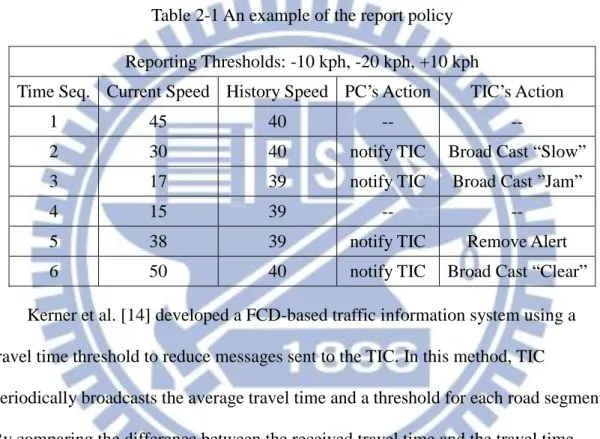
Van Buer et al. [13] proposed a notification system for reporting the traffic anomaly condition. In their system, each probe car has an on-board database to record its historical travel data, and it determines its speed anomaly during each trip. Each probe car needs to compare its historical database with its current speed, and

determine whether the speed discrepancy is greater than a predefine threshold or not. If the discrepancy satisfies the predefine threshold, probe car report its current speed to the TIC. When the TIC receives the probe car report, the TIC generates and broadcasts an alert to probe cars on the road segment. After receiving an alert from the TIC, each probe car has to compare its speed discrepancy with the alert, and report to the TIC if the speed discrepancy is greater than a predefine threshold. Table 2-1 is an example of this report policy. In step 2, the probe car detects that the speed discrepancy is equal the predefine threshold (-10 mph), and notifies the TIC that it detects anomaly changes. When the TIC receives the notification, the TIC generates

9

the “Traffic Slow” alert to all probe cars. In step 3, a probe car detects that the speed discrepancy is larger than the “Slow” alert threshold, so the probe car notifies the TIC. When the TIC receives the notification, it broadcast “Jam” alert to probe cars. The disadvantage of this method is that each probe car compares its current speed with its historic speed data. Since a probe car may be driven by different drivers with different driving behaviors, it is possible that the probe car may generate anomaly traffic data.

Table 2-1 An example of the report policy Reporting Thresholds: -10 kph, -20 kph, +10 kph

Time Seq. Current Speed History Speed PC’s Action TIC’s Action

1 45 40 -- --

2 30 40 notify TIC Broad Cast “Slow” 3 17 39 notify TIC Broad Cast ”Jam”

4 15 39 -- --

5 38 39 notify TIC Remove Alert 6 50 40 notify TIC Broad Cast “Clear” Kerner et al. [14] developed a FCD-based traffic information system using a travel time threshold to reduce messages sent to the TIC. In this method, TIC

periodically broadcasts the average travel time and a threshold for each road segment. By comparing the difference between the received travel time and the travel time record itself with the threshold, the PC decides whether or not to send a report to the TIC. The decision is based on the following equation:

∣ 𝑅_𝑘(𝑣)− 𝑅_𝑘(𝑐) ∣< 𝛥𝑅_𝑘(𝑐) (2.1)

Where 𝑅_𝑘(𝑣) is the travel time measure by probe car, 𝑅_𝑘(𝑐) is the travel time broadcasted by the TIC, and 𝛥𝑅_𝑘(𝑐) is the threshold value. The in-equality above checks if the travel time difference between the probe cars measured value and the

10

TIC broadcasted value is greater than the TIC broadcasted threshold. If the condition is satisfied, the probe car sends the traffic information report to the TIC. Using threshold values does reduce the communication cost, but the accuracy of the generated traffic information may also decrease.

Tanizaki and Wolfson [15] designed a randomized report policy to improve the threshold approach. They define server delay, which is a delay from a probe car sending reports to the TIC till the TIC broadcasts a new threshold. In this delay time interval, there may be a large amount of unanimous traffic information sent to the TIC if there are many probes traveling on the same road segment. To address this problem, when the threshold is satisfied, instead of always sending a report to the TIC, the probe sending the report with a probability p,this is determined by the TIC for each road segment to reduce the number of reports and achieve high accuracy. This reduces the volume of reports sent at the server delay interval, but may result in incomplete traffic data received by the TIC and less real-timeliness of the traffic information generated.

To deal with the issues above, Ayala et al. [16] proposed a flow-based report policy for FCD-based traffic information systems. They don’t use threshold values to determine whether to send the traveling data to the TIC or not. Every probe car has the same probability to transmit the traveling data to the TIC. The transmission

11

probability 𝑝 = 𝑘 / 𝑁, where k is the number of messages that the TIC needs to receive from probe cars in order to guarantee a given confidence in the average speed computation, and N is the estimated of the flow of vehicles through the road segment during the collection period. When a vehicle reaches the end of a road segment it computes k and N. The sample size k is compute by probes based on central limit theorem, and N is an estimate of the flow of vehicles through the road segment during the collection period. The speed-flow model chosen for the flow-based policy is Greenshields model. The relationship is given by the equation (2.2). Where d is the traffic-jam density, 𝑉_𝑏 is the average velocity of the previous collection period, and V is the free-flow speed on the given segment. The equation comes from the speed-flow relationship where flow is 0 at zero speed (𝑉_𝑏 = 0) and at free-flow speed (𝑉_𝑏 = 𝑉).

flow ≈ d ∗ 𝑉_𝑏(1 −𝑉𝑏

𝑉) (2.2) Use the equation (2.2) above, one can compute the flow throughout the collection period as equation (2.3), where τ is the length of the collection period (in seconds) [16].

N = flow ∗ τ (2.3) After computing the k and N, the probe vehicle transmits the traffic record to the TIC with probability 𝑝 = 𝑘 / 𝑁 . Compared with the threshold method, this policy generates more accurate traffic information and lowers the communication cost. This

12

method uses Greenshields model to estimate the traffic flow. However, Greenshields model is suitable for highway road segments, but unsuitable for urban roads.

Our TIS design based on the threshold model provides more accurate traffic information for urban roads according to the current trend of the traffic condition trends to reduce the number of reports sent by the probes.

13

Chpter 3 The System Design

3.1 System Overview

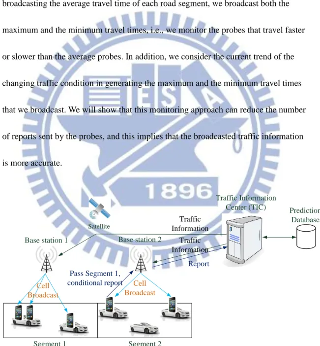
Our TIS design is based on the reporting threshold model, but instead of broadcasting the average travel time of each road segment, we broadcast both the maximum and the minimum travel times, i.e., we monitor the probes that travel faster or slower than the average probes. In addition, we consider the current trend of the changing traffic condition in generating the maximum and the minimum travel times that we broadcast. We will show that this monitoring approach can reduce the number of reports sent by the probes, and this implies that the broadcasted traffic information is more accurate.

Traffic Information

Center (TIC) _Prediction Database

Satellite

Segment 1 Segment 2

Base station 1 Base station 2

Cell Broadcast Cell Broadcast Traffic Information Report Pass Segment 1, conditional report Traffic Information

14

Fig 3-1 depicts our system architecture. Our system consists of two types of components: a Traffic Information Center (TIC) and Probe Cars (PCs). The TIC is a centralized server, which receives the traffic reports from probe cars and generates the traffic information for each road segment. In our system, a road segment is defined as the roads between two big intersections in the road network. PCs are general vehicles with people on-board carrying smart phones equipped with Global Position System (GPS) receiver and wireless communication ability, and installed our traffic

information reporting application. The smart phones receive the maximum and the minimum travel time of the traveling road segment from the TIC, and measure the traffic condition. After the smart phones passed the road segment, they send reports to the TIC if reporting conditions are met. So, there is a close-loop feedback in our system. Probe cars report their traveling data to the TIC, and based on the reports the TIC predicts the traffic information broadcasting to the probe cars.

3.2 Maximum and Minimum Travel Time

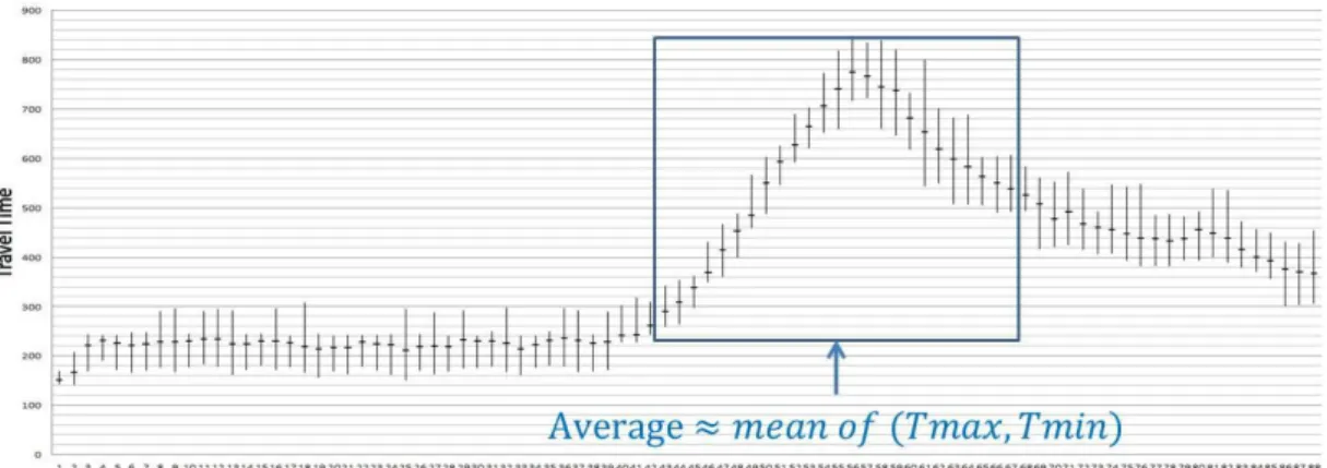
Before we design our TIS, we have used traffic simulation software to simulate traffic congestion on urban roads. Fig 3-2 shows one of the results.

15

Fig 3-2 A congestion environment analysis chart

In this experiment, the simulation time is 3 hours, and the simulated road segment is 1.6 km long. The initial input traffic flow is 1800 vehicle/hr. The input traffic flow start to increase at simulation time 1 hour, and keep increasing at 200 vehicle/hr. every 5 minutes until simulation time 1.5 hours, the largest flow is 3000 vehicle/hr. The input traffic flow starts to decrease at simulation time 1.5 hours200 vehicle/hr. every 5 minutes until the simulation time 2 hours, and back into initial flow (1800 vehicle/hr.) in the last hour. The traffic light cycle is 120 seconds. We record the maximum, minimum and the average travel times of the vehicles passing the road segment in each traffic light cycle. Each vertical stick represents the range between the maximum and the minimum travel time, and the short horizontal bar on the stick represents the average travel time. In the congestion period, we can find that the average travel time of the segment is roughly equal to the mean of the maximum and the minimum travel times. From this simulation, we can observe that it is possible to estimate the average travel time from the maximum and the minimum travel time.

16

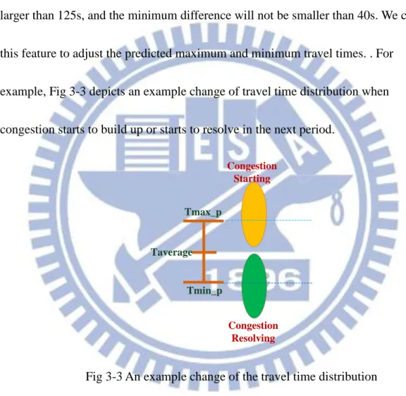
We also found that the difference between the maximum and the minimum travel times is within a stable range for plurality data; we call this range Δ. After our statistics, the value will fall in 40s to 125s, i.e. the maximum difference between the maximum travel time and the minimum travel time in a traffic light cycle will not be larger than 125s, and the minimum difference will not be smaller than 40s. We can use this feature to adjust the predicted maximum and minimum travel times. . For

example, Fig 3-3 depicts an example change of travel time distribution when congestion starts to build up or starts to resolve in the next period.

Tmax_p Tmin_p Taverage Congestion Starting Congestion Resolving

Fig 3-3 An example change of the travel time distribution

The eclipses represent the travel time distribution in the next cycle. When traffic congestion starts to build up, the travel time distribution moves up; when a congestion starts to resolve, the distribution moves down. Using conditional report thresholds, the TIC may only receive reports with travel times larger than Tmax-p when a traffic

17

congestion worsens, and receive reports smaller than Tmin-p when a traffic congestion

improves.

Compared with the conventional methods which calculate the average travel time in a time interval and provide the average travel to the probes, our method is more accurate in generating the traffic data. First, it’s difficult to obtain the accurate average travel time with a small number of probe cars. Second, using conditional report

methods to obtain the average travel time is likely to produce large errors. Fig 3-3 is an example of generating an inaccurate average at the start and the end of a

congestion using conditional report thresholds. If the traffic condition is the end of congestion, because of the conditional report, only the probe cars that travel time is less than dotted line will report their data, if we average these probes’ reports to get the average travel time, we will get the wrong value.

Generally, there are few probes whose travel times on a road segment are close to the maximum or the minimum travel time. In our design, these probes are required to send their travel times to the TIC. This would reduce the number of reports sent to the TIC significantly. In addition, when the TIC can accurately predict the maximum and the minimum travel times from the reports received, the number of reports will be further reduced, because the reporting ranges will be small by accurate predictions.

18

3.3 The System Operation

The goal of our system design is to reduce the number of traffic reports that PCs send to the TIC, while maintaining the accuracy of the traffic information broadcasted by the TIC. To achieve the goal, PCs adopt a conditional report policy, i.e., PCs send reports only when certain conditions are met. In our system, the TIC would broadcast the predicted maximum travel time (denoted Tmax-p) and the predicted minimum travel

time (denoted Tmin-p) of each road segment. When a PC travels through a road

segment, the PC compares its travel time (denoted TPC) with the maximum travel time

and the minimum travel time broadcasted by the TIC. The PC sends a report containing the traveled segment and the travel time to the TIC when TPC >

(1+α)*Tmax-p or TPC < (1-β)*Tmin-p, i.e., only the PCs that travel faster or slower than

the average are required to report. In this way, we can monitor the changes of the maximum and the minimum travel times that PCs take on a road segment. Compared with the convention TISs where PCs report periodically or when passing a road segment, this conditional report policy would reduce the number of reports sent to the TIC when there are a large number of PCs on the road network.

Second, to further reduce the number of reports sent by the PCs while

maintaining the accuracy of the traffic information broadcasted by the TIC. The TIC generates Tmax-p and Tmax-p based on the trend of the changing traffic condition. For

19

example, when the TIC detects that the traffic is slowing down; the TIC would predict larger Tmax-p and Tmin-p, so that it would keep receiving the reports of travel times from

PCs that travel faster or slower than the average. Otherwise, the TIC would not receive the reports of travel times from PCs that are faster than the average because the traffic is slowing down and no PC travels the road segment in a shorter time interval than Tmin-p.

Last, since the travel time prediction based on the trend of the changing traffic condition could be wrong, so that there is no report from PCs travel faster or slower than the average. The TIC would detect this problem and modify the Tmax-p or Tmax-p

accordingly. The modification process may repeat a couple cycles before the respective reports of travel time are received by the TIC.

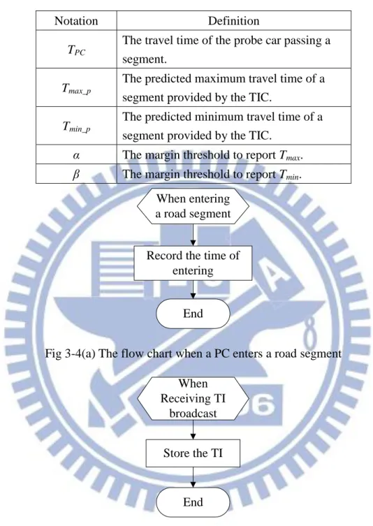
3.4 Algorithm of the Probe Car

Our probe car is designed to be an event trigger system. Table 3-1 lists notation that used in probe car system. The events that a PC system needs to deal with can be classified into three cases. First is when a PC entering a pre-defined road segment, second, when a PC receives Traffic Information (TI, Tmax-p and Tmin-p) broadcasted by

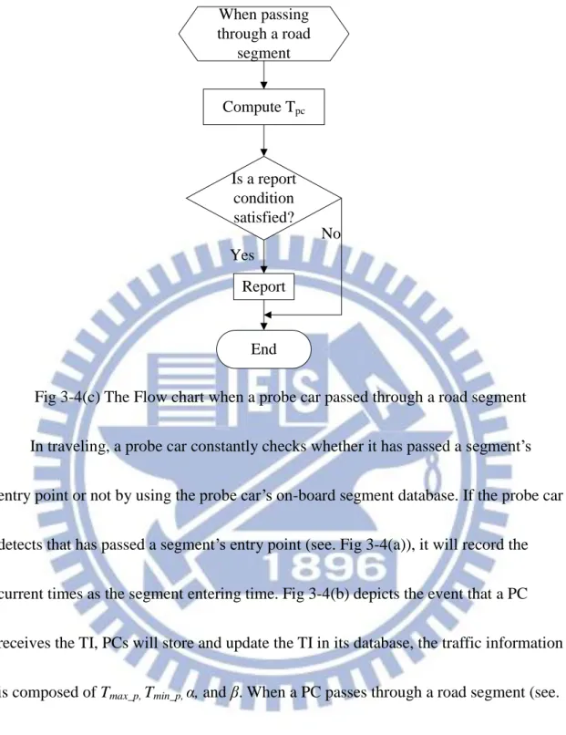
the TIC, and the last, when a PC passing through a pre-defined road segment. Figs 3-4(a) to (c) describe the flow chart of the three events above in our PCs system.

20

Table 3-1 Parameters used in the probe car system. Notation Definition

TPC

The travel time of the probe car passing a segment.

Tmax_p

The predicted maximum travel time of a segment provided by the TIC.

Tmin_p

The predicted minimum travel time of a segment provided by the TIC.

α The margin threshold to report Tmax.

β The margin threshold to report Tmin.

When entering a road segment Record the time of

entering End

Fig 3-4(a) The flow chart when a PC enters a road segment

When Receiving TI

broadcast Store the TI

End

21 When passing through a road segment Compute Tpc Is a report condition satisfied? Report Yes No End

Fig 3-4(c) The Flow chart when a probe car passed through a road segment In traveling, a probe car constantly checks whether it has passed a segment’s entry point or not by using the probe car’s on-board segment database. If the probe car detects that has passed a segment’s entry point (see. Fig 3-4(a)), it will record the current times as the segment entering time. Fig 3-4(b) depicts the event that a PC receives the TI, PCs will store and update the TI in its database, the traffic information is composed of Tmax_p, Tmin_p, α, and β. When a PC passes through a road segment (see.

Fig 3-4(c)), the PC will first compute the segment travel time TPC by using the current

time minus the entering time. After calculate TPC, the PC compare it with the Tmax_p

and Tmin_p with threshold α and β. Check if TPC > (1-α)*Tmax-p, or TPC < (1+β) Tmin-p. If

one of the conditions is satisfied, then the PC report TPC as Tmax or Tmin to the TIC.

22

3.5 Algorithm of Traffic Information Center

The TIC is designed to be an event trigger system. Table 3-2 lists notation that used in our TIC system. The events that the TIC system needs to deal with can be classified into two cases. First is when receiving Tmax (Tmin) report, second, when a

traffic light cycle ends. The Figs 3-5(a) to (b) describe the flow chart of the two events above in our TIC system.

Table 3-2 Parameters used in the TIC system. Notation Definition

Tmax

The report value of the maximum travel time

Tmin

The report value of the minimum travel time

adoption_flag A flag indicated that the report is adopted

by the TIC or not

significant_change

A flag indicated that the report has a significant difference with the prediction value

steadyArg Argument for determine the trend is steady

or not, initial = 0.05

ϒ Argument for calculate the prediction value,

initial = 1/3

AdjustArg Argument for modify the prediction value,

initial = 0.04

Δ The suitable range for Tmax_p and Tmin_p,

23

Store the report

Determine the trend

Does it match the trend?

Adopted Predict new Tmax_p (Tmin_p)

Add new Tmax_p (Tmin_p) to

prediction table

End

Non-adopted Yes

No

Set significant_change = true

Is any report significant_change == true in the previous 120

seconds No Yes No Yes When receiving Tmax (Tmin) report

% 15 (Tmin_p) Tmax_p (Tmin_p) Tmax_p -(Tmin) Tmax 

24

Broadcast the maximum Tmax_p and the minimum Tmin_p

from prediction table for each road segment End

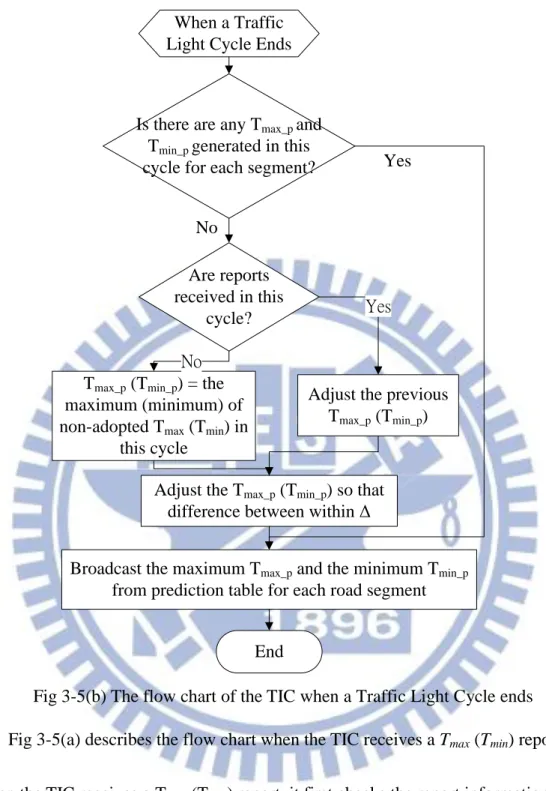
When a Traffic Light Cycle Ends

Is there are any Tmax_p and

Tmin_p generated in this

cycle for each segment? Yes

Are reports received in this

cycle? No

Tmax_p (Tmin_p) = the

maximum (minimum) of non-adopted Tmax (Tmin) in

this cycle

Adjust the previous Tmax_p (Tmin_p)

No

Yes

Adjust the Tmax_p (Tmin_p) so that

difference between within Δ

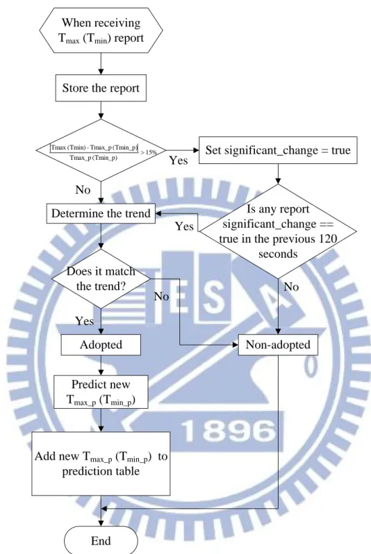
Fig 3-5(b) The flow chart of the TIC when a Traffic Light Cycle ends Fig 3-5(a) describes the flow chart when the TIC receives a Tmax (Tmin) report.

When the TIC receives a Tmax (Tmin) report, it first checks the report information (i.e. segment ID, Tmax or Tmin) and then stores the report in the corresponding reported

table. In our TIC system, each road segment has its own report table for storing Tmax

and Tmin reported by PCs. Then, the TIC checks if the Tmax (Tmin) is of significant

25

called significant_change true, checks if there is another report of significant change in the previous 120 seconds. If not, the TIC does not adopt the report and sets the report’s adoption_flag false. Otherwise, it sets the adoption_flag true and goes on to determine trend procedure. In this step, we reject an isolated report of significant change.

To determine the changing trend of traffic condition, the TIC computes 4 factors based on the reports of each traffic light cycle as follows,

M_max = The maximum of Tmax M_avg = The average of Tmax m_min = The minimum of Tmin

m_avg = The average of Tmin

Then, the TIC divides the four factors of the current cycle divides by those of the previous 2 cycle (e.g._{𝑀_max (𝑇−2)}𝑀_max (𝑇) , T denotes the current cycle), respectively, to obtain four trend factors. A threshold, steadyArg, is used to determine the trend of each trend factor; the trend may be rising, declining or stable. If a trend factor is larger than (1+

steadyArg), it indicates a rising trend. If it is smaller than (1- steadyArg), a declining

trend. Otherwise, it is a stable trend. After that, the final trend is determined by majority vote of the four trend factors.

26

the trend or not. If the report matches the trend, the TIC adopts this report, and vice versa. The conditions of adopting a report are in Table 3-3. A Tmax report is adopted

during a rising or stable trend, if it’s the maximum of all Tmax in the previous 120

seconds, but it is adopted immediately during a declining trend. A Tmin report is

adopted during a declining or stable trend, if it’s the minimum of all Tmin in the

previous 120 seconds, but it is adopted immediately during a rising trend. The TIC also sets the report’s adoption_flag accordingly. If the report is adopted, the TIC goes on to prediction procedure.

Table 3-3 The conditions of adopting a report. Adoption table

Condition Rising Trend Declining Trend Stable Trend

Tmax

maximum value in

120 seconds adopt immediately

maximum value in 120 seconds

Tmin adopt immediately

minimum value in 120 seconds

minimum value in 120 seconds In the prediction procedure, the TIC uses the average factor related to the report type (i.e. M_avg for a Tmax report and m_avg for a Tmin report to generate the predicted

Tmin-p or Tmin-p as follows.

_ = + (M_ vg( ) − M_ vg( − 2)) ∗ ϒ _ = + ( _ vg( ) − _ vg( − 2)) ∗ ϒ (3.1)

If M_avg(T-2) or m_avg(T-2) factor is not available, then the predicted value will be the reported Tmax (Tmin). After that, the TIC adds the Tmax_p (Tmin_p) to the

27

corresponding prediction table with the current timestamp.

Fig 3-5(b) shows the operation flow chart of the TIC when a traffic light cycle ends. In this event, the TIC first checks if there are any Tmax_p and Tmin_p generated in this cycle for each segment. If so, the TIC broadcasts the maximum of Tmax_p and the minimum of Tmin_p generated in this cycle for each segment. If not, the TIC checks if there are any reports received in this cycle. If so, the TIC set the new Tmax_p (Tmin_p) to

be the maximum (minimum) of the non-adopted Tmax (Tmin) in this cycle. If there is no

report in this cycle, then the TIC adjusts the previous prediction with an AdjustArg. In adjusting Tmax_p, the TIC multiplies the previous Tmax_p with (1- AdjustArg), and in

adjusting Tmin_p, the TIC multiplies the previous Tmin_p with (1+ AdjustArg). After

generating the new Tmax_p (Tmin_p), the TIC use Δ to adjust the generated value to

ensure that the difference of Tmax_p and Tmin_p is in a suitable range. After that, the TIC

28

Chpter 4 Evaluation and Analysis

4.1 Simulation Environment

We use VISSIM [17], a traffic model simulator, to develop our simulation environment. Fig. 4-1 depicts a simulated 6.8-km long urban main road, which is composed of 16 intersections with 16 branch roads. The 16 intersections evenly divide the main road into 17 small segments, each of which is 400 meters long. We collect traffic information for each 1.6-km long road segment, which is composed of 4 small segments, as the brown line and the green line depicted in Fig. 4-1. The vehicle flow will be input from the left side of the main road, and every branch also inputs vehicle flow into the main road. Starting from the entry of the main road, at every four branches 60% of the vehicles on the outer lane of the main road make right turns to the branch.

Fig. 4-1 The VISSIM simulator example

29

traffic congestion. The simulated traffic flow changes from a smooth flow to a maximum flow and finally back to smooth. In the simulation, the input flow can be divided into 4 intervals: (1) a smooth flow for 1 hour, (2) increasing the flow for 30 minutes with a flow rise every 5 minutes, (3) decreasing the flow for 30 minutes with a flow decline every 5 minutes, (4) a smooth flow for 1 hour. We have simulated 3 flow settings: light, moderate and heavy traffic flows. Table 4-1 shows the simulation parameters used in our simulation, and Table 4-2 shows the traffic flow for each setting.

Table 4-1 Parameters used in the simulation Total road length 6.8 km

Number of lanes 3

Number of segments 2

Vehicle Composition 10% probe cars, 88% regular cars, 2% vans Desired Speed Car: 40 - 60 kph (uniformly distributed)

Van: 40 - 45 kph (uniformly distributed)

Simulation time 3 hr

Traffic light cycle(120 seconds) Green Yellow Red

Main 65 s 5 s 50 s

Branch 45 s 5 s 70 s

Table 4-2 Traffic flow setting for the 3 environments Traffic flow Smooth flow Maximum flow

light 1800 veh/hr 2000 veh/hr moderate 1800 veh/hr 2500 veh/hr heavy 1800 veh/hr 3000 veh/hr

30

records of the simulated cars. Each record consists of the simulation time, the ID of a car and the car’s location. Table 4-3 list a number of location records of probe cars. The location records of probe cars are used as inputs to the emulation program of the probe cars.

Table 4-3 The partial VISSIM record of the result file. Simulation time ID of probe car Position (x-axis

coordinate) 65.0 77 18.0 66.0 49 294.0 66.0 6 393.1 66.0 3 393.2 66.0 76 33.4 66.0 34 349.0

4.2 Evaluations

We use Java programming language to develop an emulation program that implements the functions of our probe cars and the TIC; we called the emulation program TIS_Emu. We input the location records generated by VISSIM to TIS_Emu, and TIS_Emu generates reports to the TIC for each probe car, and Tmax_p and Tmin_p

based on the probe cars’ reports for the TIC.

To evaluate the performance of our system, we first check if the Tmax_p and Tmin_p

predicted by the TIC match the change of the traffic Figs. 4-2 to 4-4 plot the travel times of all vehicles and the predicted Tmax_p and Tmin_p against the simulation time.

31

Each blue square dot represents a general vehicles’ travel time, and each orange square dot represents of a probe cars’ travel time. A red square represents a Tmax_p and

a green circle represents a Tmin_p generated by TIC. Fig. 4-2 plots the results of the

light traffic flow setting (see Table 4-2), Fig. 4-3 plots the results of the moderate flow setting and Fig. 4-4 plots the results of the heavy flow setting. We can see that in every setting of flow, the predicted Tmax_p and Tmin_p generated by the TIC follow the

traffic trends properly.

For the light traffic flow (see Fig. 4-2), the travel times are divided into three groups, with most of the vehicles in the middle group and very few vehicles on the upper group. The predicted Tmax_p remains at the top of the middle group for both

segments 1 and 2. , Note that at simulation time about 4200, 6600, and 7500 seconds, there are three isolated Tmax of significant change, which do not affect the predicted

Tmax_p. We can see in both segment 1 and segment 2, the Tmin_p fluctuates around the

lower group. The reason is that the volume of vehicles in the lower group is too small and the limited sampling of the 10% probe cars may not fall in the lower group for every cycle, which leads to no Tmin report. In this case, the TIC modified the Tmin_p by

multiplying it by (1+AdjustArg) with the constraint that the difference between Tmin_p

and Tmax_p must fall in the range of . Therefore, Tmin_p fluctuates but remains in the

32

Fig. 4-2 The travel times, Tmax_p and Tmin_p at the light traffic flow.

For the moderate traffic flow (see Fig. 4-3), the Tmax_p catches the change of the

maximum travel time. We can observe that in the congestion worsening period (during simulation time 5000 to 7000 sec.), there is no Tmin report, but Tmin_p is

33

period, there is no Tmax report, but Tmax_p is properly adjusted by the Tmin reports. For

the heavy traffic flow (see Fig. 4-3), the results are similar to those of the moderate traffic flow setting.

34

Fig. 4-4 The travel times, Tmax_p and Tmin_p at the heavy traffic flow

Second, we evaluate the accuracy of the predicted Tmax_p and Tmin_p in our design.

A predicted Tmax_p (Tmin_p) is compared with the maximum (minimum) travel time of

all vehicles passing the segment after the predicted Tmax_p (Tmin_p) is broadcasted and

35

(Tmin_p) is defined to be the absolute error between the predicted Tmax_p (Tmin_p) and the

maximum (minimum) travel time of all vehicles.

For all vehicles’ experience, we count the number of vehicles whose travel time is larger than the latest broadcasted Tmax_p and the number of vehicles whose travel

time is smaller than the latest broadcasted Tmin_p. In addition, we compute the Mean

Absolute Error (MAE) between each vehicle’s travel time and the mean of the latest broadcasted Tmax_p and Tmin_p. For each flow setting; we simulate with 10 different

random seeds and average the 10 simulation results.

Tables 4-4 to 4-6 list the accuracy of the TIC’s predictions for each traffic flow setting. The simulation results indicate that the prediction errors of Tmax_p and Tmin_p

are about the same for both segments and for all three traffic flow settings. The MAE in percentage of Tmax_p fall in the range from 8.5% to 11.2%, and that of Tmin_p from

9.3% to 11.2%. For all vehicles’ experience, 20-23% of the vehicles experience a travel time larger than Tmax_p, and 5-12% experience a travel time smaller than Tmin_p.

Although the prediction errors of Tmax_p and Tmin_p are about the same, more vehicles

experience a travel time larger than Tmax_p. This does not imply we have poorer

predictions for Tmax_p. With 20 % of the vehicles whose travel time is larger than

Tmax_p and 10 % of them are probe cars, we would have 2% of all vehicles reporting

36

we have fewer vehicles reporting Tmin. In particular, during the traffic congestion

worsening period, we have almost no Tmin report, because Tmin_p is under-estimated.

The TIC can only adjust Tmin_p from Tmax_p. The MAE of using the mean of Tmax_p and

Tmin_p to predict the average travel time is in a range of 27-39 sec. or 11-13% in

percentage.

Table 4-4 Prediction accuracy for flow setting 1 (light) Prediction Error (error percentage)

Tmax_p Tmin_p

Segment 1 26.35 (9.5%) 15.73 (9.4%) Segment 2 30.3 (10.9%) 16.11 (9.3%)

All Vehicles’ Experience

number of > Tmax_p number of < Tmin_p Travel time Error

Segment 1 1210/5471 (22.0%) 387/5471 (7.0%) 29.75 (13.4%) Segment 2 1300/5934 (21.9%) 330/5934 (5.3%) 27.19 (12.3%)

Table 4-5 Prediction accuracy for flow setting 2 (moderate) Prediction Error (error percentage)

Tmax_p Tmin_p

Segment 1 29.01 (9.9%) 20.31 (10.9%) Segment 2 32.12 (10.1%) 24.87 (11.2%)

All Vehicles’ Experience

number of > Tmax_p number of < Tmin_p Travel time Error

Segment 1 1162/5728 (20.1%) 521/5728 (9.1%) 30.97 (13.0%) Segment 2 1232/6186 (20.0%) 570/6186 (9.2%) 31.77 (11.9%)

Table 4-6 Prediction accuracy for flow setting 3 (heavy) Prediction Error (error percentage)

Tmax_p Tmin_p

Segment 1 33.11 (8.5%) 31.8 (10.3%) Segment 2 34.62 (9.5%) 30.76 (10.8%)

37

number of > Tmax_p number of < Tmin_p Travel time Error

Segment 1 1302/5692 (23.0%) 678/5692 (11.9%) 39.34 (12.1%) Segment 2 1295/6102 (21.3%) 631/6102 (10.6%) 34.42 (11.1%) We also compute the communication overhead of our system. Tables 4-7 to 4-9 list the communication overhead for each traffic flow setting. We count the numbers of Tmax reports, Tmin reports and broadcast messages (BMs). The total number of PCs

passing segment 1 or 2 is about 1000 for each flow setting. About 200 PCs send Tmax

reports and 100 PCs send Tmin reports. This indicates that we reduce the number of

reports by 67% to 72%, compared with the segment-based report approach. Since the TIC broadcasts the traffic information every traffic light cycle, in three hours, TIC only broadcast 180 times for 2 segments.

Table 4-7 Communication overhead for flow setting 1 (light) Communication Overhead

number of PCs Report Max Report Min number of BMs

Total 990.3 205.2 73.4

180 Reports

reduced 72.0%

Table 4-8 Communication overhead for flow setting 2 (moderate) Communication Overhead

number of PCs Report Max Report Min number of BMs Total 1041.6 195.7 110.3

180 Reports

38

Table 4-9 Communication overhead for flow setting 3 (heavy) Communication Overhead

number of PCs Report Max Report Min number of BMs Total 1021.9 213.5 125.6

180 Reports

reduced 67.0%

At last, we investigate the effects of the penetration rate of the probes. We simulate the three flow settings with various penetration rates of probes equals, 2.5%, 5%, 10%, 20% and 40%. We compare the prediction error, the travel time error, the number of reports and the percentage of reports reduced. The results are depicted in Figs. 4-5 to 4-8.

Fig. 4-5 The prediction errors for different penetration rates of probes

0% 5% 10% 15% 2.50% 5% 10% 20% 40%

PC percentage

Prediction Error

α, β = 0 α, β = 0.04

39

Fig. 4-6 The travel time errors of different penetration rates of probes

Fig. 4-7 The number of reports for different penetration rates of probes 0% 5% 10% 15% 20% 2.50% 5% 10% 20% 40%

PC percentage

Travel Time Error

α, β = 0 α, β = 0.04 0 500 1,000 1,500 2,000 2.50% 5% 10% 20% 40%

PC percentage

Number of reports

α, β = 0 α, β = 0.04

40

Fig. 4-8 The reports reduced for different penetration rates of probes Figs 4-5 and 4-6 show that when the penetration rate of probes increases, both the prediction error and the travel time error decrease slightly. We also simulate two settings of α and β, α = 0, β = 0 and α = 0.04, β = 0.04. The results in Fig. 4-5 and 4-6 indicate that for the two settings of α and β, the prediction error and the travel time error are about the same. Fig. 4-7 shows that as the penetration rate of probes

increases, the number of reports increases significantly. In addition, the rising slop of the red line (α = 0.04, β = 0.04) is much bigger than the blue line (α = 0, β = 0). The results in Fig. 4-8 show that as the penetration rate of probes increases, the percentage of the reduced reports increases, and the reduced reports of blue line (α = 0, β = 0) is much larger than that of the red line (α = 0.04, β = 0.04).

0% 20% 40% 60% 80% 100% 2.50% 5% 10% 20% 40%

PC percentage

Reports reduced

α, β = 0 α, β = 0.04

41

Chpter 5 Conclusions

In this thesis, we propose a FCD-based traffic notification system that addresses the issue of reducing communication requirements. The system consists of a

centralized traffic information center (TIC) and a group of probe cars (PCs). The PCs can be general vehicles with people on-board carrying smart phones equipped with Global Position System (GPS) receiver and, wireless communication ability, and installed our traffic information reporting application. In our system, the TIC

generates and broadcasts the predicted maximum and minimum travel time of a road segment to PCs periodically. In the conventional FCD-based TIS, the PCs send

reports to the TIC periodically or when a road segment is traveled. In our system, only PCs that travel near the maximum or the minimum travel times are required to send reports. We have performed computer simulations to evaluate our design. The

simulation results indicate that our approach reduced the number of reports by 70% in average, compared with the conventional segment-based report policy. The prediction error of the maximum and minimum travel time on a road segment of 1.6 km is 10% in average. In addition, when using the mean of the maximum and the minimum travel time as the average travel time, the estimation error of the average travel time compared with the all vehicles’ experience is 12.3% in average.

42

In our system, the TIC needs to broadcast the traffic information periodically to the PCs. However, the broadcast function is not yet well supported by the public wireless networks, such as the UMTS, or by the vehicular communication networks, such as WAVE. Without the broadcast function, real-time traffic information cannot be efficiently delivered to all the PCs on the road network, new approaches for real-time traffic dissipation to PCs need to be studied.

43

References

[1] L. Figueiredo, I. Jesus, J. Machado, J. Ferreira, and J. Santos, “Toward the development of intelligent transportation systems”, in Proceedings of the 4th IEEE Intelligent Transportation Systems Conference, Oakland, CA, 2001, pp. 1207-1212.

[2] TomTom, http://www.tomtom.com/

[3] IntelliOne, http://www.intellione.com/

[4] ITIS Holdings plc, http://www.itisholdings.com/

[5] Mediamobile, http://www.mediamobile.com/

[6] P. T. Martin, Y. Feng, and X. Wang, “Detector technology evaluation”, Department of Civil Environmental Engineering, University of Utah-Traffic Lab, Salt Lake City, UT, 2003.

[7] D. Middleton and R. Parker, “Vehicle Detector Evaluation”, Publication FHWA/TX-03 /2119-1. Texas Transportation Institute, Texas Department of Transportation, FHWA, 2002.

[8] Prashanth Mohan, Venkata N. Padmanabhan, Ramachandran Ramjee, “Nericell: Rich Monitoring of Road and Traffic Conditions using Mobile Smartphones”, 2008

[9] H. Bar-Gera. “Evaluation of a cellular phone-based system for measurements of traffic speeds and travel times: a case study from Israel.” Transportation Research C, 15(6):380{391, 2007.

[10] Lars Wischhof, Andre Ebner, Hermann Rohling, Matthias Lott, and Rüdiger Halfmann, “SOTIS - A Self-Organizing Traffic Information System”, in

44

Proceedings of the 57th IEEE Vehicular Technology Conference, 2003.

[11] R.-P. Schaefer, K.-U. Thiessenhusen, and P. Wagner. A Traffic Information System by Means of Real-time Floating-car Data. In Proc. ITS World Congress, Chicago USA, 2002.

[12] Baik Hoh, Marco Gruteser, Ryan Herring, Jeff Ban, Daniel Work, Juan-Carlos Herrera, Alexandre M. Bayen, Murali Annavaram, Quinn Jacobson, “Virtual Trip Lines for Distributed Privacy-Preserving Traffic Monitoring”, 2008

[13] Darrel J. Van Buer, Son K. Dao, Xiaowen Dai, et al., “Traffic Notification System for Reporting Traffic Anomalies Based on Historical Probe Vehicle Data”, US 7460948, 2008.

[14] B. Kerner, C. Demir, R. Herrtwich, S. Klenov, H. Rehborn,M. Aleksic, and A. Haug, “Traffic State Detection with Floating Car Data in Road Networks”, in IEEE Proc. on Intelligent Transportation Systems, 2005.

[15] M. Tanizaki and O. Wolfson, “Randomization in Traffic Information Sharing Systems,” in GIS ’07: Proc. of the 15th annual ACM Intl. Symp. on Advances in Geographic Information Systems, 2007.

[16] Daniel Ayala, Jie Lin, Ouri Wolfson, Naphtali Rishe, and Masaaki Tanizaki, “Communication Reduction for Floating Car Data-based Traffic Information Systems”, 2010 Second International Conference on Advanced Geographic Information Systems, Applications, and Services Communication, 2010.