A support vector machine approach to CMOS-based radar signal processing for vehicle classification and speed estimation

(1)

Contents lists available atSciVerse ScienceDirect

Mathematical and Computer Modelling

journal homepage:www.elsevier.com/locate/mcm

A support vector machine approach to CMOS-based radar signal

processing for vehicle classification and speed estimation

Hsun-Jung Cho

∗

, Ming-Te Tseng

Department of Transportation Technology and Management, National Chiao Tung University, Taiwan

a r t i c l e i n f o Keywords:

Vehicle detector Radar signal CMOS

Support vector machine Speed

Classification Optimization

a b s t r a c t

In this work, a complementary metal-oxide semiconductor (CMOS) based transceiver with a sensitivity time control antenna is successfully implemented for advanced traffic signal processing. The collected signals from the CMOS radar system are processed with optimization algorithms for vehicle-type classification and speed determination. The high recognition rate optimization algorithms are mainly based upon the information of short setup time and different environmental installation of each sensor. In the course of optimization, a video recognition module is further adopted as a supervisor of support vector machine and support vector regression. Compared with conventional circuit-based detector systems, the developed CMOS radar integrates submicron semiconductor devices and thus not only possesses low stand-by power but also is ready for production. In the meantime, the developed algorithm of this study simultaneously optimizes the vehicle-type classification and speed determination in a computationally cost-effective manner, which benefits real-time intelligent transportation systems.

Accurate, economic methods of collecting traffic information are essential in an intelligent transportation system (ITS). Traffic data has been gathered primarily via inductive loop detectors, pneumatic road tubes, and temporary manual counts [1,2]. However, traffic detectors developed recently use video, sonic, ultrasonic, radar or infrared energy [3–5]. These detectors are non-intrusive and mounted either overhead or to the side of traffic lanes. Considering the cost, radar and video sensors both have multi-lanes capability. A single detector of either of these types can detect up to eight or ten lanes. However, poor weather conditions, such as snow and heavy rain, can seriously impact video sensors. In contrast, radar sensors still function effectively in poor weather. Therefore, radar sensors are a good choice in ITS applications owing to their multi-lane coverage and resistance to weather impacts.

Motorcycles are a major transportation mode in many Asian countries, including Taiwan, Malaysia and Vietnam. However, the mixing of motorcycles and other traffic is hazardous. The key step to overcome this problem is to know the flow information of motorcycles. Currently, most radar detection algorithms classify vehicles into three or five categories, but generally exclude motorcycles from the classification system. Well designed radar hardware can be used in conjunction with a classification algorithm to detect motorcycles. This study thus illustrates a radar sensor classification scheme that classifies vehicles into four categories: motorcycles, small, medium and large vehicles.

Considering radar hardware, frequency-modulation continuous-wave (FMCW) is the main technology used by radar sensors to support multi-lane capabilities. The two most popular methods for making FMCW sensor transceivers at microwaves and millimeter waves are hybrid microwave integrated circuits and the GaAs monolithic microwave integrated

∗_{Corresponding author. Fax: +886 3 5710657.} E-mail address:[email protected](H.-J. Cho).

(2)

Table 1

The specifications of radar sensor. Height 4–7 m Central frequency 10.5 GHz Band width 50 MHz Pulse repeat frequency 1500 Hz Down range resolution 3 m Max range 60 m Max range shift frequency 30 KHz Elevation angle/Azimuth angle 50°/20°

ADC 200 KHz

FFT 128 points

circuit chipset. This investigation tests the vehicle classification and speed estimation for a new FMCW radar incorporating a complementary metal-oxide semiconductor (CMOS) transceiver [6,7] with an equivalent sensitivity time control (STC) planar antenna. Comparing to traditional hybrid integrated circuit radar, the CMOS radar is ready for production, cost-effective, miniaturized and consumes low power. This is the reason why this work develops CMOS radar. The planar antenna adds attenuation in the receiver as a function of time, and thus reduces the near-field interference by a factor of one over some power of the range. Restated, the antenna incorporates a STC function. This study reports, to the best of the authors’ knowledge, the first X -band CMOS sensor with a uniformly distributed signal-to-noise ratio for monitoring multiple-lane traffic. One contribution of this study is to prove that the first X -band CMOS radar vehicle detector does detect motorcycles and vehicles accurately in ITS.

A radar vehicle classifier [8,9] has two general constraints: short setup time and different environmental installation of each sensor. Since the environmental installation of a radar sensor strongly impacts vehicle radar cross section (RCS), the features of vehicles will depend on the environmental installation of sensors. It is difficult to include all possible installation data in training a classifier. A supervised classifier is difficult to collect training data for all environmental installation conditions. Because the traffic managers hope to reduce the influence of traffic conditions, the setup time should be as short as possible. When the setup time is short, the collected training data will be skewed in categories. Traffic volume may include numerous small cars, few buses and trucks during the short training period. The unsupervised classifier will have poor recognition rates in skewed data. Therefore, traditional supervised or unsupervised classifiers are hard to apply directly for the sensor under these two constraints. Hence, vehicle classifications for roadside radars are in a gray area where two types of classifiers can’t be applied directly. The important contribution of this work is to combine support vector machine (SVM) with a video system to overcome this drawback.

Numerous classifiers have been developed and tested for data cluster or pattern recognition [10], and these classifiers are categorized into two types: supervised and unsupervised. In supervised learning, the aim is to learn a mapping from the input to an output whose correct vehicle classes are provided by a supervisor. In unsupervised learning, there is no such supervisor and we only have input of data. K -means cluster is a famous unsupervised classifier that has been used for numerous applications. Furthermore, SVM [11,12] and linear discriminant analysis (LDA) [13,14] are two supervised classifiers. LDA was originally developed in 1936 by R.A. Fisher. SVMs have been used for isolated handwritten digit recognition, object recognition, speaker identification and face detection in images. To find the optimal classifier, this study tests these three classifiers under two constraints. Vehicle speed is estimated using a virtual loop concept [1,2,15] that requires vehicle and virtual loop length to make an estimate. Support vector regression (SVR) is used to predict vehicle length, while a video calibrating system is used to measure virtual loop length. A skew training dataset and numerous classification scenarios are used to test the classifiers. Finally, the results are analyzed and compared.

The remainder of this paper is organized as follows. Section2introduces the radar system and introduces the radar system and considers the proposed vehicle classification technique and the speed estimation method. Test results demonstrating the system performance are then presented in Section3. Finally, conclusions are presented in Section4.

2. Vehicle classification and speed estimation

In this section, the radar system is first introduced and the requirements of the radar sensor are also presented in Section2.1. The algorithm of vehicle classification and speed estimation will be shown in the following subsections. 2.1. Radar system

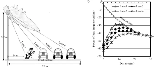
To support multi-lane capabilities, the FMCW radar detector is designed for roadside installation, as illustrated inFig. 1(a). The radar’s height is the same as that of general poles, namely from 4 to 7 m. The central frequency is 10.5 GHz. The vehicle width leads the radar with 50 MHz band width and 3 m down range resolution. The radar is designed to cover a maximum of eight lanes, and can be positioned a maximum of 60 m from the roadside. The total frames per second, or the pulse repeat frequency, are 1500 Hz. Therefore, the max range shift frequency is 30 kHz. The corresponding signal processing speed for ADC is 200 kHz. Furthermore, the elevation and azimuth angles of the planar antenna are 50°and 20°. The specifications of the radar system are summarized inTable 1.

(3)

a

b

Fig. 1. (a) Installation of radar sensor. There are four lanes. The sensor is installed at a height of 5.2 m above the ground and at a distance of 14 m from the

first lane. The maximal distance is 32 m of the sensor from the most distant lane. (b) The echo power distribution for each lane of road. The echo power of each lane is near-constant from the distances 14 to 32 m. The dashed line is a curve that fits the echo power distribution of the vehicle on the road surface.

Fig. 2. Block diagram of the proposed X -band FMCW sensor system [6,7], comprising two external antenna arrays, a single-chip CMOS transceiver (enclosed by the dashed line) and an external digital signal processing unit along with the necessary electronics. A power amplifier is added to increase output power level.

The building blocks of the X -band FMCW of the radar are shown inFig. 2. Dual planar antenna arrays are located at the transmitter output and the receiver input. The planar antennas have an equivalent STC function. As shown inside the dashed lines, the radio frequency transceiver is a chip based on a standard 0

.

18

µ

m CMOS technology [6,7]. The CMOS transceiver performs most of the required RF signal processing. A power amplifier is added to increase output power. Furthermore, a baseband digital signal processing unit is used for instantaneous and simultaneous assessment of range measurements.

Fig. 1(b) illustrates the beat frequency power distribution of the antenna corresponding to the installation inFig. 1(a). There are four echo power curves for four lanes. Generally, the echo power of most antennas decays at a rate 1

/

R4_{. For this specially} designed planar antenna, the shorter range power decay can be cancelled by the near field interference. The dashed line, shown inFig. 1(b), is the road surface curve. Restated, the echo power of the vehicle signal will stay on the four inter-points of the road surface curve. The empirical results, illustrated in Section3, show that complementing the magnitude of the vehicles with the second power of the frequency can obtain an accurate vehicle classification rate.

2.2. Algorithm

The RCS of a vehicle is the key information used in vehicle classification and speed estimation.Fig. 3shows a sample RCS signal of a car received from the installation ofFig. 1(a). The profile of a vehicle signal resembles a mountain, and different vehicles create different shaped mountains. The vehicle classifier extracts features from the profiles and classifies vehicles accordingly. The speed estimator also identifies features from the profiles and calculates the vehicle speed. Vehicle RCS is

(4)

a

b

Fig. 3. (a) A picture of a vehicle passing through the detection area of a radar detector. The closed area indicated by a dashed line is the detection area of

the radar detector. (b) The spectrogram of the vehicle is shown in (a).

influenced by radar height and angle, radar distance from the first lane, vehicle speed, vehicle shape and vehicle distance to radar. Most of these factors are only fixed on the completion of the radar sensor installation. Restated, the vehicle profiles were completely changed when the environmental installation was adjusted. This is a constraint for the supervised classifier, which needs to be retrained for each new environmental installation. Generally, traffic managers hope that sensor setup minimally impacts traffic conditions. It means that the sensor setup time must be minimized. The setup time influences the learning time and learning data of a classifier. If a training classifier is provided, the learning data is gathered during setup. Short setup time results in a skewed distribution of vehicle types. The number of cars may be large while the number of trucks is low. This forms the second constraint: short training time and skewed training data.

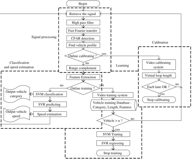
Fig. 4presents an overview of an algorithm for these two constraints. The algorithm includes four phases, namely signal processing, calibration, learning and ‘classification and speed estimation’. After retrieving the radar signal, a high pass filter is applied to filter background clutter signals. Fast Fourier transformation is used to get the range profiles of vehicles on lanes. Then, constant false alarm rate (CFAR) thresholds are used to detect the presence of vehicles. If calibrating work is needed, the video calibrating system will be used to calibrate the virtual loop lengths. When the calibrating job is finished, the vehicle profiles will be complemented by the range of vehicle. The aim is to let vehicles have the same signal gains in different lanes. The next step is to extract nine features from the complemented vehicle profile. While the training job has never been done before, these features will be saved in a vehicle training database. The category and length of vehicle, which is the output of the video recognition system, will be saved into the training database, too. If the number of vehicles is bigger than a threshold, SVM and SVR will finish the learning step. When the learning job is done, SVM will use vehicle features to classify a vehicle’s category. Finally, SVR will predict the length of the vehicle and output the vehicle speed. The details of the algorithm will be presented in the following subsections. The pseudocode of the algorithm is shown as follows. Void Vehicle_classifier_and_speed_estimation_algorithm() begin while true Signal_processing(); if need calibrating Calibrating(); endif if vehicle

<

n Feature_extracting(); endif if need training Learning() endif if training done Vehicle_classification_and_speed_estimation(); endif endwhile End void Signal_processing() begin

(5)

Online training ? Retrieve the signal

High pass filter Fast Fourier transfer

CFAR detection

Feature Extraction

SVM Traning SVM classification

SVR regressing SVR predicting Vehicle training Database :

Category, Length, Features Video traning system

Vehicle > n ? Output vehicle

[

n

]

is retrieved from the time

domain during a pulse interval t. Each discrete signal frame has 128 points (n

=

1

· · ·

128), and there are a total of 1500 signal frames per second (pulse repeating frequency

=

1500). Since noise and background clutter disturb the normal vehicle echo signals, a simple high pass filter H

(

z

) =

1

−

z−1is used to cancel the background clutter. The filtered signal yt

[

n

]

is

shown in Eq.(1):

yt

[

n

] =

xt

[

n

] −

xt−1

[

n

]

.

(1)

Furthermore, the high pass filter can also emphasize the movement of vehicles. Since a high magnitude of some frequencies means that some vehicles present on some lanes, a fast Fourier transform (FFT) is performed on yt

[

n

]

to get the frequency

domain data Yt

[

n

]

. That is to say, when a vehicle is presented at distance 3

∗

n m at time t

, |

Yt

[

n

]|

is greater than some

threshold. To avoid false alarms of vehicle presence, the clutter-map constant false alarm rate (CFAR) [16] technique is adopted. The basic characteristic of clutter-map CFAR is that the false alarm probability remains approximately constant in clutter by a dynamic threshold. Vehicles with an echo power exceeding the threshold thus can still be detected. Eq.(2)

shows the clutter-map CFAR threshold for the range n during pulse t:

Tt

[

n

] =

α (γ × |

Yt−1

[

n

]| +

(

1

−

γ ) × |

Yt−2

[

n

]|

)

(2) where

α =

2 and

γ =

0

.

9.

The final step in signal processing is to collect the vehicle profile Vt

[

m

]

presented at m-th range bin Yt

[

m

]

during the

time interval in which the vehicle is present in the detection area. All classification methods are based on the vehicle profile from which features are extracted. Eq.(3)defines the profile of the vehicle signal. Each magnitude of m-th range bin

|

Yt

[

m

]|

is multiplied by power k of range frequency fmto compensate for the decay of received power:

Vt

[

m

] = |

Yt

[

m

]| ×

fmk (3)

where T1

<

t

<

T2and T1and T2are the first and last detection times of a vehicle which passes through the radar detection area.

(7)

2.2.2. Feature extraction

Nine features need to be extracted from the vehicle profile, most of which are based on the physical characteristics of the vehicle. First, the energy of the vehicle profile is shown in Eq.(4). A large vehicle implies large RCS, which in turn means high energy. Squared energy is used to emphasize this characteristic. Other features are obtained from the statistical parameters associated with the vehicle magnitude profile. These features include the maximal, mean and mean square error for elements of Vt

[

m

]

: Energy

=

T2



t=T1 Vt

(

m

).

(4)

Another physical phenomenon of vehicles is the vibration of the vehicle profile. Small vehicles have low vibration while large vehicles have high vibration. Eq.(5)calculates vehicle vibration. To increase the weighting of these characteristics, the square of vibration is used. The vibration is just used to do mathematical differentiation and the energy is the same concept as doing mathematical integration. These features of each vehicle profile form a point in the feature space:

Vibration

=

T2



t=T1

|

Vt

(

m

) −

Vt−1(m

)|.

(5)

2.2.3. Learning and classification

This section aims to identify a classifier for effectively classifying vehicles into one of four categories: motorcycles, small, medium and large.

First, this study tries the K -means clustering (denoted as K -means). K -means is one of the best known data clustering methods. The goal of k-means is to find k points of a dataset that best represent the dataset in a certain mathematical sense. These k points are also known as cluster centers. After obtaining these cluster centers, they can be used for data classification. Here K -means is used as a method of partitional clustering in which the numbers of clusters and random centers are specified before starting the clustering process. The number of clusters is set to four. An objective function is then defined as the sum of the squared distances between a point in a feature space and the nearest cluster centers. The standard K -means procedure is then followed to minimize the objective function iteratively by finding a new set of cluster centers. These cluster centers can reduce the value of the objective function at each iteration. Here the maximal iteration is set to 10.

The next classifier is LDA, which is a supervisory classifier. LDA obtains a linear transformation (‘‘discriminant function’’) of the two predictors, X and Y , which yields a new set of transformed values that provides more accurate discrimination than either predictor alone. A transformation function is found that maximizes the ratio of between-class to within-class variance. The transformation seeks to rotate the axes so as to maximize the differences between the groups when the categories are projected on the new axes. In the ideal case, a projection can be found that completely separates the categories. However, in most cases no transformation exists that provides full separation, so the objective is to obtain the transformation that minimizes the overlap among the transformed distributions. The LDA can be derived as a plug-in Bayes classifier. LDA projects the nine feature dimensional space considered in this study into a three dimensional linear discriminant (LD) space. The plug-in classifier finds the average group centers for each vehicle category and saves it. When predicting a test sample vehicle, the classifier measures the Mahalanobis distance between the group center and the LD projected point of the vehicle features. The plug-in classifier then estimates the posterior probability of each group using the Mahalanobis distance, the prior probability which is the group probability of the training set, and the covariance matrix. The testing vehicle belongs to the group with the highest posterior.

The last classifier is SVM, which is also a supervisory classifier. SVMs attempt to identify a set of support vectors, two support hyperplanes, and an optimal hyperplane for separating two groups. SVM is a binary classifier. Two strategies can be developed to support multiple classifications: one-against-one and one-against-rest. The one-against-rest strategy constructs k SVMs to separate k groups. The m-th SVM separates the m-th group from the others. For k groups, the one-against-one strategy constructs k

(

k

−

1

)/

2 SVMs to separate each pair of groups. This study tests SVM using the one-against-one approach, in which six SVMs are constructed, each of which trains data from two different vehicle groups. Prediction is performed by voting, where each classifier makes a prediction and the most frequently predicted class wins (‘‘Max Wins’’). In cases where two groups receive an identical number of votes, this study simply selects the one with the smallest index.

For supervisory classifiers LDA and SVM, the environmental installation problem leads to retraining of the classifier for each installation of the radar sensors. To resolve the problem, this study proposes a learning method based on a video training system, as shown inFig. 5. Using clutter-map CFAR, the radar system can know the in and out time of a vehicle. When the radar system sends vehicle-in or vehicle-out triggers to the video system, the video system immediately captures a video frame. These two video frames can then be used to perform image processing to obtain the vehicle type. The vehicle type and its features are saved in a training database which can be used to train a supervisory classifier.

2.2.4. Calibration and speed estimation

The vehicle speed is estimated using Eq.(6). The detection zone of each lane forms a virtual loop. The key to correctly estimating the speed is to more precisely calculate the three parameters of Eq.(6):

(8)

Fig. 5. Video training and calibrating system. The system receives vehicle-in and vehicle-out triggers when a vehicle is either inside or outside the detection

area. After receiving the triggers, the system captures two video frames. The image processing unit then outputs virtual loop length, vehicle category and vehicle length.

Table 2

Set of vehicles used to test the classifier.

Motorcycle Small Medium Large Total 30 145 12 4

Speed

=

Lv

+

Lz

∆T

,

(6)

where L_v denotes the length of the vehicle, Lz represents the length of the virtual loop and ∆T is the time of vehicle

occupation.

It is easy to obtain the vehicle occupation time from clutter-map CFAR. The length of the virtual loop must be carefully calibrated. The length of the virtual loop is also an environmental installation problem. The length differs between environmental installations. Theoretically, the virtual loop length can be obtained from radar equations, antenna patterns, and the height and angle of the radar sensor. However, these methods are imprecise and inconvenient. A more accurate method is to take measurements in the field.Fig. 5presents a video calibrating system for measuring the virtual loop length via image processing. Based on clutter-map CFAR, the times at which the vehicle is either in or outside of the virtual loop can be derived. The video calibrating system can obtain two video frames at a time. Image processing can be performed to obtain the distance of vehicle movement between the two frames. The moving distance exactly equals the virtual loop length. SVR is used to estimate the vehicle length. SVR is almost the same as SVM, with one difference being that the optimal hyperplane is used to predict values in SVR, while in SVM it is used to separate classes. Since SVR is still a supervised regression method, the video system is still required to measure the vehicle lengths and save them in the training database.

3. Results and discussion

Table 2lists a dataset to train two classifiers: SVM and LDA. Generally, users require installing the radar sensor as soon as possible. During the short setup time, the numbers of vehicle in four categories is skewed. A good classifier requires an acceptable classification rate, after applying its learning algorithm to skew data constraints. The training data satisfies the short setup time and skew data constraints.

After applying the K -means, LDA and SVM to the training data inTable 2, the classification rate is 42%, 93% and 94%, respectively. The rate results in K -means not being a good classifier in situations involving constraints. The LDA and SVM have a near identical leave-one-out recognition rate, and moreover this rate is acceptable. Both methods are good classifiers, and can resolve any associated environmental installation problems. The following paragraphs analyze and compare these two classifiers in more detail (seeTable 3).

(9)

Table 3

The classification rate of classifiers.

K -means LDA SVM

42% 93% 94%

Table 4

Vehicles obtained from the field.

Category Motorcycle Small Medium Large Type ID 1 2 3 4 5 Type Motorcycle Car Van Bus Truck Subtotal 30 79 66 12 4 Total 191

Table 5

Leave-one-out recognition rate for different classifiers and categories.

Category LDA(fm) SVM(fm) LDA(fm2) SVM(fm2) LDA(fm4) SVM(fm4)

1 vs. 2 vs. 3 vs. 4 vs. 5 73% (140/191) 76% (145/191) 76% (146/191) 82% (156/191) 78% (149/191) 71% (136/191) 1 vs. 2345 95% (182/191) 98% (187/191) 96% (183/191) 99% (189/191) 94% (180/191) 97% (186/191) 1 vs. 23 vs. 4 vs. 5 93% (177/191) 94% (180/191) 95% (181/191) 98% (186/191) 93% (178/191) 93% (177/191) 23 vs. 45 96% (155/161) 97% (156/161) 97% (156/161) 99% (159/161) 96% (154/16) 96% (155/161) 23 vs. 4 vs. 5 96% (155/161) 96% (155/161) 98% (158/161) 98% (158/161) 96% (154/161) 95% (153/161) 2 vs. 3 vs. 4 vs. 5 72% (116/161) 75% (121/161) 75% (121/161) 80% (128/161) 76% (123/161) 71% (115/161) 2 vs. 3 76% (110/145) 75% (109/145) 77% (112/145) 79% (114/145) 78% (113/145) 74% (108/145) 4 vs. 5 88% (14/16) 94% (15/16) 88% (14/16) 94% (15/16) 94% (15/16) 100% (16/16)

Table 4lists another testing dataset that meets the short setup time and skew data constraints. The test data were obtained from a field site on a road in Chu-Pei City, Taiwan. The radar is installed as illustrated inFig. 1. The same traffic volume can be collected on a normal urban road within a 10–15 min period. The five vehicle types from the table can be classified into four categories. All vehicles from different lanes are merged into a single training dataset. According to the radar equation, in Eq.(7), the receiver power of the vehicle is decayed by 1

/

R4_{. As shown in}_{Fig. 1}_{(b), the planar antenna} is specially designed to perform an SPC function which compensates for the decay in each lane. The receiver power of the road surface, indicated by the dashed line curve, resembles a curve with some power of the range. Therefore some software STC functions are tested, as shown in Eq.(3), to compensate for the decay of the road surface. Before extracting the features from the vehicle profile, the amplitude of the profile is multiplied by some power of the frequency. Although the classifier is designed to classify vehicles into four categories, recognition rates remain an area of interest for numerous combinations of different vehicle types:

Pr

=

PtG2

λ

2

σ

(

4

π)

3_R4

,

(7)

where Prdenotes receiver power, Ptrepresents transmitter power,

λ

is wavelength, G denotes antenna gains,

σ

represents

RCS, and R is vehicle range.

Table 5lists the test results for different powers of frequency for SVM and LDA. The highlighted cells represent the highest leave-one-all recognition rates for different categories. SVM wins almost all scenarios in fm2cases.Table 6lists the

error matrix for a SVM

(

fm2

)

case. Therefore, by compensating the received signal with power two of the frequency, SVM can

obtain the best recognition rate. The first row, ‘‘1 vs. 2 vs. 3 vs. 4 vs. 5’’, indicates a low recognition rate for each classifier. This low rate means that creating excessively narrow categories will result in a low recognition rate. Comparing the third and fifth rows, ‘‘1 vs. 23 vs. 4 vs. 5’’ and ‘‘23 vs. 4 vs. 5’’, reveals that the recognition rates are almost equal in the same classifier. Motorcycles can generally be separated from other vehicle types. The second row, ‘‘1 vs. 2345’’, confirms this. Examining the last two rows, ‘‘2 vs. 3’’ and ‘‘4 vs. 5’’, reveals that cars and vans are difficult to separate, while buses and trucks can generally be separated.

Table 7shows the calibrated virtual loop length which is output from the video calibrating system. The far lane is slightly longer than the near lane. The planar antenna design is responsible for this effect.Fig. 6shows the vehicle length output by SVR. The estimated truck lengths are shorter than the visually measured lengths obtained from the video system, and the estimated motorcycle lengths are longer than the visually measured ones (seeFig. 6(b)). The reason is that the total number of vans and cars is 75%. The training data is skewed, leading SVR to make length predictions for all vehicles that are close to those of cars.Fig. 7describes the vehicle speed. Since the estimates of motorcycle length are high, the motorcycle speed always exceeds that of visual measurements obtained using the video system (seeFig. 7(b)). The situation for trucks is the reverse of the above, with estimates of length and speed being lower than the visual measurements.

(10)

Table 6

Leave-one-out error matrix for SVM(fm2).

Detect vehicle class Actual vehicle class

Motorcycle Small Medium Large Motorcycle (1) 29 1 0 0 Small (2, 3) 1 143 1 0 Medium (4) 0 1 11 1 Large (5) 0 0 0 3 Total 30 145 12 4 Error (%) 3 1 8 25 Recognition rate (%) 98 Length(m) Vision Detect Length(m) Vision Detect 16 14 12 10 8 6 4 2 0 1 11 21 31 41 51 Vehicle number

a

5 4 3 2 1 0 1 2 3 4 5 6 7 8 9 10 11 12 Motorcycle number

b

Fig. 6. Vehicle output lengths from SVR. The open triangles with dashed lines denote the lengths measured from the video calibrating system. Meanwhile,

the rectangles with black lines represent the estimated lengths obtained using the proposed algorithm. (a) The vehicle lengths were output from SVR. (b) The motorcycle lengths output from SVR.

Speed(km/h) Vision Detect Speed(km/h) 120 100 80 60 40 20 0 1 11 21 31 41 51 Vehicle number 3 4 1 2 5 6 7 8 9 10 11 12 13 14 15 Motorcycle number 90 80 70 60 50 40 30 20

a

b

Vision Detect

Fig. 7. Estimated vehicle speeds. The open triangles with dashed line are the speeds measured from the video system. The rectangles with black line are

the speeds estimated using the proposed algorithm. (a) Estimated speeds for all vehicle categories. (b) Estimated speeds for motorcycles.

Table 7

Virtual loop length for each lane.

Lane1 Lane2 Lane3 Lane4 Virtual loop length 7.9 m 8. 1 m 9.2 m 9.9 m

4. Conclusions

In this study, a CMOS based transceiver with STC antenna has been successfully implemented for advanced traffic signal processing. The collected signals from the CMOS radar system have been processed with developed optimization algorithms for vehicle-type classification and speed determination. The high recognition rate optimization algorithms are mainly based upon the information of short setup time and different environmental installation of each sensor. The algorithm includes four phases, namely signal processing, calibration, learning and ‘classification and speed estimation’. In the calibration and learning phases, a video recognition module has been further adopted as a supervisor of SVM and SVR. SVM has successfully classified vehicles into four categories: motorcycles, small, medium and large vehicles in the classification phase. SVR has estimated vehicle lengths and determined their speeds accurately in the speed estimation phase. Specially, the proposed algorithm can detect motorcycles and estimate their speeds precisely. Compared with conventional circuit-based detector systems, the developed CMOS radar integrates submicron semiconductor devices and thus not only possesses low stand-by power but also is ready for production. In the meantime, the algorithm has successfully provided a high recognition rate in a gray area where traditional unsupervised classifiers have low recognition rates and supervised classifiers are hard to prepare training data. Furthermore, the developed algorithm of this study simultaneously optimizes the vehicle-type classification and speed determination in a computationally cost-effective manner, which benefits real-time intelligent transportation

(11)

system. In the future, enhanced vehicle length and speed accuracy can be obtained by applying SVR to each category of vehicles. Another direction for future research could be to apply the SVM model to vehicle signals of each lane.

Acknowledgments

The authors would like to thank the National Science Council of Taiwan (Contract Nos. 98-2221-E-009-104 and 99-2221-E-009-091-MY2) for financially supporting this research.

References

[1] W.-H. Lin, J. Dahlgren, H. Huo, An enhancement to speed estimation using single loop detectors, Proceeding of Intelligent Transportation Systems 1 (2003) 417–422.

[2] J.J. Reijmers, On-line vehicle classification, IEEE Transactions on Vehicular Technology 29 (1980) 156–161.

[3] G. Palubinskas, H. Runge, Radar signatures of a passenger car, IEEE Geoscience and Remote Sensing Letters 4 (2007) 644–648.

[4] I. Urazghildiiev, R. Ragnarsson, P. Ridderstrom, A. Rydberg, E. Ojefors, K. Wallin, P. Enochsson, M. Ericson, G. Lofqvist, Vehicle classification based on the radar measurement of height profiles, IEEE Transactions on Intelligent Transportation Systems 8 (2007) 245–253.

[5] G. Alessandretti, A. Broggi, P. Cerri, Vehicle and guard rail detection using radar and vision data fusion, IEEE Transactions on Intelligent Transportation Systems 8 (2007) 95–105.

[6] S. Wang, H.-S. Wu, C.-H. Chang, C.-K. Tzuang, Modeling and suppressing substrate coupling of RF CMOS FMCW sensor incorporating synthetic Quasi-TEM transmission lines, in: IEEE MTT-S International Microwave Symposium, 2007, pp. 1939–1942.

[7] C.-K. Tzuang, C.-H. Chang, H.-S. Wu, S. Wang, S.X. Lee, C.C. Chen, C.Y. Hsu, K.H. Tsai, J. Chen, An X -band CMOS multifunction-chip FMCW radar, in: IEEE MTT-S International Microwave Symposium, 2006, pp. 2011–2014.

[8] S.-J. Park, T.-Y. Kim, S.-M. Kang, K.-H. Koo, A novel signal processing technique for vehicle detection radar, Microwave Symposium Digest 1 (2003) 607–610.

[9] J.M. Munoz-Ferreras, F. Perez-Martinez, J. Calvo-Gallego, A. Asensio-Lopez, B.P. Dorta-Naranjo, A. Blanco-del-Campo, Blanco-del-Campo, Traffic surveillance system based on a high-resolution radar, IEEE Transactions on GeoScience and Remote Sensing 46 (2008) 1624–1633.

[10] K. Fukunaga, Introduction to Statistical Pattern Classification, Academic Press, San Diego, California, USA, 1990.

[11] P.-F. Pai, System reliability forecasting by support vector machines with genetic algorithms, Mathematical and Computer Modelling 43 (2006) 262–274.

[12] Q. He, Z.-Z. Shi, L.-A. Ren, E.-S. Lee, A novel classification method based on hypersurface, Mathematical and Computer Modelling 38 (2003) 395–407. [13] L. Edler, J. Grassmann, S. Suhai, Role and results of statistical methods in protein fold class prediction, Mathematical and Computer Modelling 33

(2001) 1401–1417.

[14] J. Duchene, S. Leclercq, An optimal transformation for discriminant and principal component analysis, IEEE Transactions on PAMI 10 (1988) 978–983. [15] H.-S. Lai, H.-C. Yung, Vehicle-type identification through automated virtual loop assignment and block-based direction-biased motion estimation,

IEEE Transactions on Intelligent Transportation Systems 1 (2000) 86–97.