Scattering of water wave by a submerged horizontal plate and a submerged permeable breakwater

Scattering of water wave by a submerged

horizontal plate and a submerged permeable

breakwater

Hu-Hsiao Hsu, Yung-Chao Wu

Department of Civil Engineering, National Chiao-Tung University, Hsinchu, Taiwan Received 12 July 1997; accepted 15 October 1997

Abstract

Based on a two-dimensional linear water wave theory, this study develops the boundary element method (BEM) to examine normally incident wave scattering by a fixed, submerged, horizontal, impermeable plate and a submerged permeable breakwater in water of finite depth. Numerical results for the transmission coefficients are also presented. In addition, the numeri-cal technique’s accuracy is demonstrated by comparing the numerinumeri-cal results with previously published numerical and experimental ones. According to that comparison, the transmission coefficient relies not only on the submergence of the horizontal impermeable plate and the height of the permeable breakwater, but also on the distance between horizontal plate and permeable breakwater. Results presented herein confirm that the transmission coefficient is minimum for the distance approximately equal to four times the water depth.1998 Elsevier Science Ltd. All rights reserved.

Keywords: Boundary element method; Submerge horizontal plate; Submerge permeable breakwater; Transmission coefficient; Reflection coefficient; Linear friction coefficient

1. Introduction

Offshore structures, both submerged horizontal plate and submerged breakwater, are generally used to protect harbours, inlets, and beaches from wave action. In such

* Corresponding author.

0029-8018/99/$—see front matter1998 Elsevier Science Ltd. All rights reserved. PII: S 0 0 2 9 - 8 0 1 8 ( 9 7 ) 1 0 0 3 2 - 4

cases, a minimum transmission coefficient is of priority concern in their design. In general, submerged structures are advantageous in that they are less expensive than a subaerial breakwater. Moreover, they do not obstruct the ocean view, which is critical for recreational and residential shore development.

Previous investigations have treated the two-dimensional scattering of linear water waves by thin rigid plates in several manners. Burke (1964) analytically solved wave scattering by a submerged horizontal plate in deep water using the Wiener-Hopf technique. Siew and Hurley (1977) employed the method of matched asymptotic expansions to solve the problem of a submerged horizontal plate in shallow water. Patarapanich (1984a, b) applied the finite element and calculated the reflection and transmission coefficients for a submerged horizontal plate from deep to shallow-water limits. McIver (1985) considered the scattering of surface waves by a moored, submerged, horizontal plate, using eigenfunction expansions within the finite domain. Parson and Martin (1992) solved the problem of wave scattering by a submerged, horizontal plate, using a hypersingular integral equation for the discontinuity in the potential across the plate.

Wave propagation over various two-dimensional underwater permeable structures has been widely studied. A model describing wave transformation over a submerged breakwater or sill is a prerequisite in coastal design. Several investigators have addressed this problem with different subsequent models. Wave transmission, reflec-tion and energy dissipareflec-tion have been experimentally studied by Dick and Brebner (1968), Dattatri et al. (1978) and Seelig (1980). Sollitt and Cross (1972), Madsen (1974) and Madsen (1983) considered the dissipation of wave energy inside rec-tangular, emerged and porous structures under normal wave incidence. Sulisz (1985) resolved the problem for an arbitrary cross-section and Dalrymple et al. (1991) util-ized the eigenfunction method, demonstrating that for oblique waves incident upon a vertical porous structure, the reflection and transmission coefficients are significantly altered. Rojanakamthorn et al. (1989, 1990) presented a mathematical model based on linear wave theory for a rectangular submerged breakwater and extended the solution to derive a modified mild-slope equation, including wave breaking, to evalu-ate wave transformation over a trapezoidal porous breakwevalu-ater. Losada (1991) derived a similar linear model to examine monochromatic wave transformation over and through porous beds or on a submerged rectangular structure, including oblique inci-dence. Losada et al. (1996a, b) developed a linear model based on the theory of Sollitt and Cross (1972) for waves in porous media, in which the analysis focused primarily on the hydrodynamics induced inside and outside a submerged porous structure under oblique incoming regular wave trains.

In this study, we adopt the boundary element method (BEM) to treat the wave scattering problem by a fixed, submerged, horizontal impermeable plate and a sub-merged permeable breakwater under normal wave incidence. To increase the numeri-cal solution’s accuracy, the linear element is used to perform computation. To con-firm the numerical solution’s accuracy, the numerical solutions for the transmission coefficient by a fixed, submerged, horizontal plate are compared with the experi-mental results of Dick and Brebner (1968) and the numerical solutions of Patarapan-ich (1984a, b). Moreover, the numerical solutions for the reflection coefficient by a

submerged permeable breakwater are compared with the experimental results of Lee and Huang (1996).

2. Theoretical formulation of the problem

Consider a horizontal impermeable plate located above a trapezoidal permeable breakwater submerged in a water depth, h, as shown in Fig. 1. The distance is Lt

between horizontal plate and permeable breakwater. The system is idealized as two-dimensional. A Cartesian coordinate is chosen with the origin located at the still water surface. The incident wave is specified propagating in the +x direction with a wave height H and a period T.

By separating the flow field into two regions, i.e. a plate-water region (⌽1) and a porous structure region (⌽2), under the assumption of irrotational motion and an incompressible fluid outside and inside the porous structure (Sollitt and Cross, 1972), the Laplace equation must hold in every region.

ⵜ2⌽

j =0; j=1,2 (1)

The velocity potentials ⌽j(x,z,t) can be expressed as

⌽j(x,z,t)=Real[␾j(x,z)e−

i␻t_{] (2)}

where i= √ −1, ␻ denotes the wave frequency. The frequency ␻ must satisfy the dispersion relation

␻2=_{gktanh(kh) (3)}

where g represents the gravity acceleration, and k is the wave number. The velocity V → j is defined as V → j = −ⵜ⌽j (4)

whereⵜ denotes the gradient operator. The velocity potential must satisfy the follow-ing boundary conditions:

1. The free surface boundary condition (Dean and Dalrymple, 1984): ∂␾1

∂z =

␻2

g ␾1on z=0 (5)

2. The boundary condition at the water bottom: ∂␾j

∂→n

=0 on z= −h; j=1,2 (6)

i.e. the bottom is impermeable. Where n→ represents the unit normal vector point-ing out of the computation domain.

3. The boundary condition on the horizontal plate: ∂␾1

∂→n

=0 on Sm (7)

i.e. the normal velocity is zero on the solid boundary, where Smis the submerged

surface of the horizontal plate.

4. The radiation conditions:This condition expresses the behaviour of an outgoing wave at W¯ distance away from the porous structure.

5. The matching boundary conditions:Since the solutions in adjacent regions must be continuous at each interface, continuity of mass flux and pressure must be satisfied at the interfaces. In terms of the velocity potentials these conditions can be expressed as

∂␾1 ∂x =⑀

∂␾2

␾1=(S−if)␾2 (9) where ⑀ denotes the porosity of the permeable material, S represents the virtual mass coefficient and f is the linearized friction coefficient (Sollitt and Cross, 1972).

Furthermore, the solution of the system of equations requires a known value for the linearized friction coefficient f. To evaluate f an additional condition is necessary. In line with Sollitt and Cross (1972), the Lorentz’s (1926) hypothesis of equivalent work can be assumed. In doing so, f can be evaluated from the following equation,

f = 1 ␻

再

冕

冕

冕

冕

冎

where␯ denotes the kinematic fluid viscosity, Cfrepresents the turbulence drag

coef-ficient, Kp is the intrinsic permeability of the porous medium and q denotes the real

part of the seepage velocity. In addition, Kp and Cfare related to the type of porous

structure considered and are taken as given. Above parameters can be evaluated a priori experimentally and f is calculated by iterations.

The reflection and transmission coefficients of the linear water wave are defined as Kr=

Hr

H Kt= Ht

H (11)

where Hr and Ht represent the reflected and transmitted wave heights respectively.

3. BEM formulation

The boundary element method (BEM) has been used to solve a variety of problems in theoretical hydrodynamics and elasticity theory (Brebbia and Dominguez, 1989). For a boundary value problem in which the free space Green’s function, i.e. funda-mental solution, is known, the BEM can be used to perform computations only on the boundary of the domain. The effective dimensionality of the problem is reduced by one. Averting detailed computations inside the domain allows the BEM method to be more efficient than the domain type methods.

To utilize the BEM, the boundary value problems must be initially converted into an integral equation representation. Using Green’s second identity

冕

冕

where Q denotes fundamental solution of the governing equation, ⌫ represents the boundary of the solution domain,⍀ is the solution domain, and␾ denotes the velo-city potential at a selected point of the boundary.

Because the governing equation of the fluid domain is Laplace equation, the funda-mental solution is (Greenberg, 1971)

Q = 1 2␲ln

冉

1

r

冊

in which r represents the distance from the source point to the field point. From Eq. (12) any velocity potential␾ˆmof the boundary is given by

− ␤ 2␲ ␾ˆm=

冕

冉

冊

in which m is the source point, and␤ denotes the internal angle of the source point m. The integration of Eq. (14) is then carried out numerically, using Gaussian quadra-ture.

The numerical procedure of the BEM involves dividing the boundary into N seg-ments or eleseg-ments. To increase the numerical result’s accuracy, the linear element is used to perform computation on the boundary of the domain. Therefore the values

of␾ and ∂␾/∂→n at any point on the element can be defined in terms of their nodal

values and two linear interpolation functions.

For a well-posed boundary value problem, either ␾ or ␾n or a relation between

them is known at all points of the boundaries. Since both␾ and ␾n at the radiation

boundaries are unknowns, the relation between ␾ and ␾n can be constructed by

using the matching conditions of velocity and pressure, at interface AB (Fig. 1) (Wu, 1987), i.e. ␾1=␾ r=gH 2␻ cosh[k(h + z)] cosh kh e ik(x + W¯ + b_t) +gHr 2␻ cosh[k(h + z)] cosh kh e −ik(x + W¯ + b_t) +

冘

冘

The subscript of␾1denotes flow region. Hrrepresents the wave height of reflection

wave. km and␻ must satisfy the following relation.

␻2= −_gk

mtan(kmh) m=1,2,…,⬁ (17)

The relation between velocity,␾1, and normal velocity, ␾1n, on the vertical inter-face AB is derived in Appendix A, Eq. A(3) and, in the present context, can be written as: ␾1=H g ␻ cosh k(h + z) cosh kh + cosh k(h + z) ikQ0

冕

冘

冕

Similarly, on the vertical interface CD(x=(W¯ + bt)), one can obtain

␾1=␾ t=gHt 2␻ cosh[k(h + z)] cosh kh e ik(x−W¯ −b_t) +

冘

冘

␾1 and ␾1non the interface CD can be established as (see Appendix A) ␾1= cosh k(h + z) ikQ0

冕

冘

冕

The discretized forms of the radiation boundaries are established on the basis of the linear element. Rearranging in such a manner that all unknowns are taken to the left hand side and all the knowns are move to the right side leads to

[A][X]=[B] (22) where [X] denotes the vector of unknown ␾ and ∂␾/∂n, [B] represents the known vector, and [A] is the matrix of coefficients. The fact that a sufficient number of equations are available to solve unknown quantities accounts for why Eq. (22) can be solved by using the Gauss elimination method.

At corners the flux at both sides may not be unique (so called corner point). To consider the possibility that the flux at a point before a corner (not necessarily a corner point) may be different from the flux at a point after a corner, two nodes are taken at every corner in the proposed model. That is the corner node is replaced by two different nodes inside each of the two adjacent elements.

4. Numerical results and discussion

This study has developed the boundary element method (BEM) to examine the problem of scattering by a fixed, submerged, horizontal impermeable plate and a submerged permeable breakwater in water of constant depth. To our knowledge, no analytical or numerical method has been able to resolve this problem, and no experi-mental data in previous literature are available either. To ensure the current

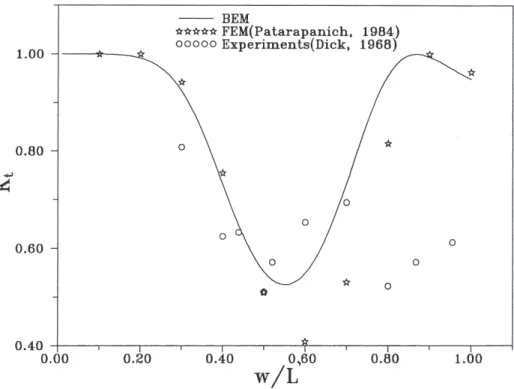
compu-Fig. 2. Comparison of transmission coefficient obtained by FEM and experiments. (d/h=0.2, t¯/h=0.1, h/L=0.2, h=0.3 m).

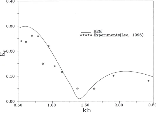
tation’s accuracy, the numerical solutions for the transmission coefficient by a fixed, submerged, horizontal impermeable plate, are compared with the experimental results of Dick and Brebner (1968) and the numerical solutions of Patarapanich (1984a); Patarapanich, (1984b)). Fig. 2 plots those results. According to this figure, L⬘ denotes the wave length above the submerged plate. The comparisons indicate that the current numerical results of linear BEM have the same trend as other scholars’ results. There-fore, the numerical solutions for the reflection coefficient by a submerged permeable breakwater are compared with the experimental results of Lee and Huang (1996), as plotted in Fig. 3. As this figure reveals, the numerical of the present for normal wave incidence correlate reasonably well with the experimental data of Lee and Huang (1996). In this case, the submerged breakwater is a homogeneous, isotropic and rectangular structure (i.e. S0=0, b/h=1.268, h¯/h=0.505). The medium proper-ties are⑀ = 0.678, Kp = 3.37 ×10−9 m2, Cf =0.047 and S =1.015. The kinematic

fluid viscosity (␯) is 1.12 ×10−6 _m2_/s.

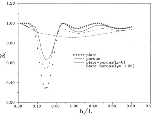
Fig. 4 displays the transmission coefficient (Kt) of a horizontal submerged

imper-meable plate located above trapezoidal submerged porous breakwater for Lt=0 and

Lt = − 1.0h, as compared with the results of a submerged horizontal impermeable

plate and a submerged porous breakwater. The plate’s geometry is w = 2.0h, d = 0.2h, t¯=0.04h and the water depth h =1.0 m. The porous breakwater’s geometry is b=0.2h, S0 =1.5, h¯=0.4h and the water depth h =1.0 m. The porous materials

Fig. 3. Comparison of reflection coefficient obtained by experiments. (b/h=1.268, h¯/h=0.505, Kp=

3.37×10−9_m2_{, C}

Fig. 4. Transmission coefficient Ktversus relative depth, h/L. Influence of the distance, Lt. (b/h=0.2,

h¯/h=0.4, Kp=1.0572×10−7m2, Cf=0.295,⑀=0.439, S=1.0,␯=1.0126×10−6m2/s, S0=1.5, w/h

=2.0, d/h=0.2, t¯/h=0.04, h=1.0 m).

characteristics are⑀=0.439, Kp=1.0572×10−7m2, Cf=0.295 and S=1.0. Herein,

only this kind of porous material is considered. The kinematic fluid viscosity (␯) is 1.0126×10−6 _m2_{/s. Comparing with the results of Fig. 4 reveals that a horizontally} submerged impermeable plate located above a trapezoidal submerged porous break-water is improving in Kt. In the following, the important effect of this distance (Lt)

on the Kt is closely examined. Because the geometry is symmetrical, only the case

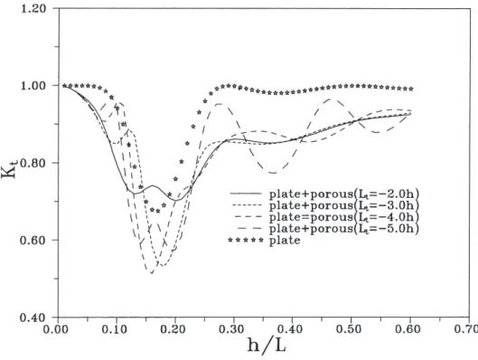
of Lt⬍ 0 is considered herein. Fig. 5 displays the variation of Ktwith relative depth

h/L for Lt = − 2.0h, Lt= − 3.0h, Lt = − 4.0h and Lt = −5.0h (w =2.0h, d = 0.2h,

t¯=0.04h, b = 0.2h, h¯=0.4h, S0 = 1.5, h = 1.0 m). According to this figure, Kt

markedly decreases with an increasing distance (Lt). As Fig. 5 reveals, increasing

distance (Lt) denotes a reduction in wave transmission taking a minimum value in

Lt ⬇ − 4.0h. Fig. 6 depicts the variation of the transmission coefficient, Kt with

relative depth h/L for given geometry (w = 2.0h, d = 0.2h, t¯=0.04h, b = 0.2h, h¯=0.5h, S0 =1.5, h =1.0 m) and the same porous material parameters (⑀=0.439,

Kp = 1.0572 × 10−

7 _m2_{, C}

f = 0.295, S = 1.0). As this figure reveals, Kt gradually

decreases with an increasing distance (Lt). The minimum Kt is in Lt⬇ −4.0h.

Fig. 7 presents the transmission coefficients, for given geometry (w = 2.0h, d = 0.3h, t¯=0.04h, b = 0.2h, h¯=0.4h, S0 = 1.5, h = 1.0 m), as a function of relative

Fig. 5. Transmission coefficient Ktversus relative depth, h/L. Influence of the distance, Lt. (b/h=0.2,

h¯/h=0.4, Kp=1.0572×10−7m2, Cf=0.295,⑀=0.439, S=1.0,␯=1.0126×10−6m2/s, S0=1.5, w/h

=2.0, d/h=0.2, t¯/h=0.04, h=1.0 m).

depth, h/L. Fig. 8 displays the variation of the transmission coefficient, Ktfor given

geometry (w= 2.0h, d =3.0h, t¯=0.04h, b= 0.2h, h¯=0.5h, S0 = 1.5, h =1.0 m). Therefore, according to Figs. 7 and 8, the oscillation of the transmission coefficient, Ktwith relative depth h/L for Lt= −5.0h. Those figures also indicate that increasing

distance (Lt) denotes a reduction in wave transmission taking a minimum value in

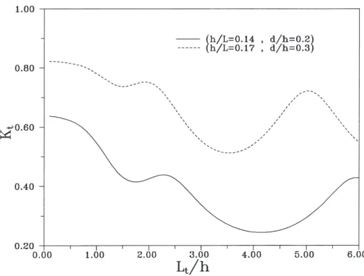
Lt ⬇ −4.0h. Fig. 9 depicts the variation of the transmission coefficients with Lt/h

for given geometry (w = 2.0h, t¯=0.04h, b = 0.2h, h¯=0.4h, S0 = 1.5, h = 1.0 m) and two different computational conditions (d/h=0.2, h/L=0.14 and d/h=0.3, h/L =0.17). From Fig. 9, we can infer that the transmission coefficient is minimum for the distance approximately equal to four times water depth (Lt ⬇ 4.0h).

5. Conclusions

The BEM with linear element has been established to examine the problem of scattering by a fixed, submerged, horizontal, impermeable plate above a submerged permeable breakwater under normal wave incidence. Comparing numerical results with previously published results and experimental results demonstrates the

numeri-Fig. 6. Transmission coefficient Ktversus relative depth, h/L. Influence of the distance, Lt. (b/h=0.2,

h¯/h=0.5, Kp=1.0572×10−7m2, Cf=0.295,⑀=0.439, S=1.0,␯=1.0126×10−6m2/s, S0=1.5, w/h

=2.0, d/h=0.2, t¯/h=0.04, h=1.0 m).

cal technique’s accuracy. The transmission coefficient, Kt, relies not only on the

submergence of the horizontal impermeable plate (d) and the height of the porous breakwater (h¯), but also on the distance between horizontal plate and porous break-water (Lt). Moreover, increasing distance (Lt) denotes a reduction in wave

trans-mission taking a minimum value in Lt ⬇ −4.0h.

Acknowledgement

The authors are grateful for financial support from National Science Council of Taiwan, R.O.C., under Grant number NSC-86-2611-E-009-003.

Appendix A

Accordingly, the matching conditions provide continuity of pressures and horizon-tal velocities normal to the vertical interface AB we can establish

Fig. 7. Transmission coefficient Ktversus relative depth, h/L. Influence of the distance, Lt. (b/h=0.2, h¯/h=0.4, Kp=1.0572×10−7m2, Cf=0.295,⑀=0.439, S=1.0,␯=1.0126×10−6m2/s, S0=1.5, w/h =2.0, d/h=0.3, t¯/h=0.04, h=1.0 m). ␾1=␾r= gH 2␻ cosh[k(h + z)] cosh kh + gHr 2␻ cosh[k(h + z)] cosh kh +

冘

冘

between ␾1 and␾1non the interface AB can be established as

␾1=H g ␻ cosh k(h + z) cosh kh + cosh k(h + z) ikQ0

冕

Fig. 8. Transmission coefficient Ktversus depth, h/L. Influence of the distance, Lt. (b/h=0.2, h¯/h=0.5, Kp=1.0572×10−7m2, Cf=0.295,⑀=0.439, S=1.0,␯=1.0126×10−6m2/s, S0=1.5, w/h=2.0, d/h =0.3, t¯/h=0.04, h=1.0 m). −

冘

冕

冕

冕

冕

Fig. 9. Transmission coefficient Ktversus Lt/h. (b/h=0.2, h¯/h=0.4, Kp=1.0572×10−7m2, Cf=0.295, ⑀=0.439, S=1.0,␯=1.0126×10−6_m2_{/s, S} 0=1.5, w/h=2.0, t¯/h=0.04, h=1.0 m). Qm=

冕

Similarly, on the vertical interface CD, we can establish

␾1=␾ t=gHt 2␻ cosh[k(h + z)] cosh kh +

冘

冘

␾1= cosh k(h + z) ikQ0

冕

冘

冕

in which Ht= 2␻ cosh (kh) igkQ0

冕

冕

Brebbia, C.A., Dominguez, J., 1989. Boundary Elements: An Introductory Course. McGraw-Hill, New York.

Burke, J.E., 1964. Scattering of surface waves on an infinitely deep fluid. J. Math. Phys. 5, 805–819. Dalrymple, R.A., Losada, M.A., Martin, P.A., 1991. Reflection and transmission from porous structures

under oblique wave attack. J. Fluid Mech. 224, 625–644.

Dattatri, J., Raman, H., Shankar, J.N., 1978. Performance characteristics of submerged breakwaters. In: Proceedings of 16th Coastal Engineering Conference, Hamburg. ASCE, New York, pp. 2153–2171. Dean, R.G., Dalrymple, R.A., 1984. Water Wave Mechanics for Engineers and Scientists. Prentice-Hall,

Englewood Cliffs, New Jersey.

Dick, T.M., Brebner, A., 1968. Solid and permeable submerged breakwaters. In: Proceedings of 11th Coastal Engineering Conference, London. ASCE, New York, pp. 1141-1158.

Greenberg, M.D., 1971. Application of Green’s Function in Science and Engineering. Prentice-Hall, New Jersey.

Lee, J.F., Huang, S., 1996. Wave interaction with submerged porous structures. In: Proceedings of 18th Chinese Conference on Coastal Engineering, pp. 273-282 (in Chinese).

Lorentz, H.A., 1926. Report of The State Committee Zuidersee 1918-1926. Den Haag, Alg, Landsdrukkerij, Dutch Text.

Losada, I.J., 1991. Estudio de la propagacio´n de un tren lineal de ondas por un medio discontinuo. Ph.D. Thesis, Universidad de Cantabria (in Spanish).

Losada, I.J., Silva, R., Losada, M.A., 1996a. 3-D Non-breaking regular wave interaction with submerged breakwaters. Coastal Engineering 28, 229–248.

Losada, I.J., Silva, R., Losada, M.A., 1996b. Interaction of non-breaking directional random waves with submerged breakwaters. Coastal Engineering 28, 249–266.

Madsen, O.S., 1974. Wave transmission through porous structures. J. Waterway, Port, Coastal, Ocean Engng Div., ASCE 100, 169-188.

Madsen, P.A., 1983. Wave reflection from a vertical permeable wave absorber. Coastal Engineering 7, 381–396.

McIver, M., 1985. Diffraction of water waves by a moored, horizontal, flat plate. J. Engng Math. 19, 297–319.

Parson, N.F., Martin, P.A., 1992. Scattering of water waves by submerged plate using hypersingular integral equations. Applied Ocean Research 14, 313–321.

Patarapanich, M., 1984a. Maximum and zero reflection from submerged plate. J. Waterway, Port, Coastal, Ocean Engng, ASCE 110, 171–181.

Patarapanich, M., 1984b. Forces and moment on a horizontal plate due to wave scattering. Coastal Engin-eering 8, 279–301.

Rojanakamthorn, S., Isobe, M., Watanabe, A., 1989. A Mathematical model of wave transformation over a submerged breakwater. Coastal Engng Japan 32, 209–234.

breakwater. In: Proceedings of 22nd Coastal Engineering Conference, Delft. ASCE, New York, pp. 1060-1073.

Seelig, W.N., 1980. Two-dimensional tests of wave transmission and reflection characteristics of labora-tory breakwaters. Tech. Report No. 80-1. U.S. Army Coastal Engineering Research Center, Fort Belvoir, Va.

Siew, P.F., Hurley, D.G., 1977. Long surface waves incident on a submerged horizontal plane. J. Fluid Mech. 83, 141–151.

Sollitt, C.K., Cross, R.H., 1972. Wave transmission through permeable breakwaters. In: Proceedings of the 13th International Conference on Coastal Engineering, vol. III, pp. 1837-1846.

Sulisz, W., 1985. Wave reflection and transmission at permeable breakwaters of arbitrary cross section. Coastal Engineering 9, 371–386.

Wu, Y.C., 1987. Analysis of wave fields generated by a directional wavemaker. Coastal Engineering 11, 241–261.