THE SEARCHING OVER SEPARATORS STRATEGY TO SOLVE SOME NP-HARD PROBLEMS IN SUBEXPONENTIAL TIME

Algorithmica (1993) 9:398-423

Algorithmica

9 1993 Springer-Verlag New York Inc.

The Searching over Separators Strategy To Solve

Some NP-Hard Problems in Subexponentiai Time x

Ro Z. H w a n g , 2 R. C. C h a n g , 3'4 a n d R. C. T. Lee 2'4

Abstract. In this paper we propose a new strategy for designing algorithms, called the searching over separators strategy. Suppose that we have a problem where the divide-and-conquer strategy can not be applied directly. Yet, also suppose that in an optimal solution to ~his problem, there exists a separator which divides the input points into two parts, A d and Cd' in such a way that after solving these two subproblems with Ad and Cd as inputs, respectively, we can merge the respective subsotutions into an optimal solution. Let us further assume that this problem is an optimization problem. In this case our searching over separators strategy will use a separator generator to generate all possible separators. For each separator, the problem is solved by the divide-and-conquer strategy, ff the separator generator is guaranteed to generate the desired separator existing in an optimal solution, our searching over separators strategy will always produce an optimal solution. The performance of our approach will critically depend upon the performance of the separator generator: It will perform well if the tota! number of separators generated is relatively small. We apply this approach to solve the discrete Euclidean P-median problem (DEPM), the discrete Euclidean P-center problem (DEPC), the Euclidean P-center problem (EPC), and the Euclidean traveling salesperson problem (ETSP). We propose O(n ~ algorithms for the DEPM problem, the DEPC problem, and the EPC problem, and we propose an O(n ~ algorithm for the ETSP problem, where n is the number of input points. Key Words. Computational geometry, NP-hardness.

1. Introduction. T h e d i v i d e - a n d - c o n q u e r strategy is a w e l l . k n o w n a p p r o a c h to designing efficient a l g o r i t h m s (Aho et al., 1976; P r e p a r a t a a n d Shamos, t985; H o r o w i t z a n d Sahni, 1978; Bentley, 1976, 1980). T h e basic idea of this a p p r o a c h is as follows:

(1) W e divide the i n p u t d a t a i n t o two subsets Ad a n d Ca.

(2) We t h e n recursively solve the two s u b p r o b l e m s with An a n d Cd as i n p u t data, respectively.

(3) Finally, we find a n efficient way to merge the s o l u t i o n s to the two s u b p r o b t e m s i n t o the s o l u t i o n to the original one.

A typical example is the closest-pair problem, which is defined as follows: given a set of n p o i n t s in the plane, find the closest pair of these points. W e c a n solve this p r o b l e m by the d i v i d e - a n d - c o n q u e r a p p r o a c h . First, we find a m e d i a n line

1 This research work was Partially supported by the National Science Council of the Republic of China under Grant NSC 79-0408-E007-04.

2 Institute of Computer Science, National Tsing Hua University, Hsinchu, Taiwan, Republic of China. 3 Institute of Computer Science, National Chiao Tung University, Hsinchu, Taiwan, Republic of China. 4 Academia Sinica, Taipei, Taiwan, Republic of China.

which divides the data into two subsets of equal size. We then find the closest pairs in An and Ca, respectively. Let the distance of the closest pair in A n (resp. Cn) be denoted as d, (resp.

db),

and d = min(d,,

db).

To find the closest pair of the entire set, we only have to examine the points in the strip which centers at the median line with 2" d as its width. F o r more details, consult Bentley (1976) and Preparata and Shamos (1985).

Many problems can be solved by the divide-and-conquer strategy (Horowitz and Sahni, 1978). It usually yields efficient polynomial algorithms. Unfortunately, not every problem can be solved efficiently by the divide-and-conquer approach. One of the reasons is that we cannot easily divide the input data into two unrelated subsets, such that the two subproblems with these two subsets as inputs can be solved independently and the solution later merged into an optimal solution.

In this paper we point out that there may exist cases characterized by the following properties:

(1) The problem is an N P - h a r d problem. Thus it is quite unlikely that it can be solved by the divide-and-conquer strategy directly.

(2) On the other hand, as far as an optimal solution S is concerned, there exists a separator, called B. The separator B divides the input data D into two parts An and Ca. Then the final solution can be derived by merging the optimal solutions to subproblems A a and Ca.

(3) The separator B has some kind of characteristic. All possible separators with such properties can be generated efficiently.

If a problem has the above properties, then although it cannot be solved by the divide-and-conquer strategy, it can be solved by

the searching over separators

strategy

which we now propose and explain in the following:

Let us further assume that our problem is an optimization problem, and we are looking for an optimal solution with the minimum cost. The searching over separators strategy works as follows:

The Searching over Separators Strategy

Input:

A set of input data D.

Output:

An optimal solution S and its cost C. Step Step Step Step Step Step Step Step Let us P points 1. Let C : = oo.

2. Use some procedure, called Procedure A, to generate all possible separators.

3. For each possible separator B, do:

4. Use B to divide the input data D into two subsets An and C d. 5. Recursively solve the subproblems with A n and C n as inputs,

respectively. Let the solutions be A s and C s, respectively. 6. Merge A S and C~ into S'. Let C' be the cost associated with S'. 7. tf C > C', then S : = S', C : = C'.

8. Return solution S as an optimal solution and the optimal cost C. consider a case where we are given a set of n points and we are to select out of them to form an optimal solution. A straightforward approach is

400 R.Z. Hwang, R. C. Chang, and R. C. T, Lee

tooxamino

..oro (;).o siblo

Therefore, the time complexity of this straightforward approach is at least

Now suppose that we apply the searching over separators strategy to solve this problem. Let

T(n,

P) be the time complexity of solving this problem by using the searching over separators approach. Assume that the separator B has some kind of characteristic, such that, after dividing, the time complexity of each subproblem is bounded by

T(n, ~.P)

and the total number of possible separators and the time needed to generate these separators are both bounded by

O(nC"/g),

Where 0 < e < 1 and c is some constant. Then we have the following formula:

T(n, P) <_ O(n c'/~) . 2" T(n, c~ . P)

<_ O(nC"/g" 2"n~"J~'g), 2" T(n,

e 2 . p ) = O(n~'/~a +~/g))-2 9

T(n, c~Z:P)

<_ O(n ~ ~,~(1 +,/;+,/~+...~)

< O(n~

Compared with the straightforward approach, the searching over separators strategy achieves a better performance.

In order for the above searching over separators strategy to work. Procedure A must be able to produce the particular separator B existing in an optimal solution as described above. If it does, the searching over separators strategy is guaranteed to have examined an optimal solution and correctly present it as a solution.

In this paper we show that the searching over separators strategy can be used to solve four geometry problems: the discrete Euclidean P-median problem (DEPM), the discrete Euclidean P-center problem (DEPC), the Euclidean P-center problem (EPC), and the Euclidean traveling salesperson problem (ETSP).

This paper is organized as follows: In Section 2 we solve the D E P M problem and the D E P C problems. In Section 3 we extend the method in Section 2 to sotve the E P C problem. In Section 4 we solve the E T S P problem. Finally, the concluding remarks are stated in Section 5.

2. The Algorithm To Solve the Discrete Euclidean P-Median Problem and the Discrete Euclidean P-Center Problem

2.1. Preliminaries.

The E P M problem is defined as follows: given n demand points on the plane, the E P M problem is to select P locations as supply points, such that the sum of distances from all demand points to their respective nearest

supply points is minimized. The D E P M problem is its related problem, in which the supply points must be selected from the set of the given demand points. There are many real-world applications of the D E P M problem. One of these applications is to choose P locations to build warehouses, such that the sum of distances from all stores to their respective nearest selected warehouses is minimized.

Formally we can formulate the D E P M problem as follows: given a set D =

{dr, d2,..., dn}

of demand points, find a set S of P supply points from the set of demand points, to minimize the following cost function:

dieD

where

l(di, s j)

is the Euclidean distance between

di

and

sj.

Megiddo and Supowit (1984) proved that the E P M problem is an NP-hard problem. Papadimitriou (1981) proved the NP-hardness of the D E P M problem.

The D E P M problem can be solved by enumerating all possible combinations of P points as the supply points and selecting the set of points which minimizes the total sum of distances from the n demand points to their respective nearest supply points. This approach takes

O(P. n P+ 1)

time (Papadimitriou, 1981). In this paper we solve the D E P M problem in

O(n ~

time.

2.2. The Generalized Discrete Euclidean P-Median Problem.

For reasons which will become clear later, we try to solve a generalized version of the D E P M problem instead of the original problem. Let us now modify the original D E P M problem into

the 9eneralized discrete Euclidean P-median problem (GDEPM).

The G D E P M problem is defined as follows: given a set D of n demand points, a set fl ~ D of fixed supply points, and the number P, we have to select a set S of P supply points from D, where fl and S are disjoint, such that

I min

{l(di, sj)}t

is minimized. di~Dks:~S~fl )

To distinguish the different problems, we use the GDEPM-(P, D, fl) problem to denote the G D E P M problem with P, D, fi as inputs.

We can immediately see that the original D E P M problem is a special case of the G D E P M problem in which fl is an empty set. Note that we have to distinguish two kinds of supply points. Thus, throughout the rest of this paper, we use fi to denote the set of the fixed supply points, and use S to denote the set of the unfixed supply points.

Essentially, we show that, for an optimal solution S to the G D E P M problem, there exists a cycle, named

the B-cycle.

Let B s c S denote the set of unfixed supply points in the B-cycle. The B-cycle has the following properties:

(1) fBs[ is no more than x/8 .(P + 3). (Note that [Bs[ denotes the number of points in the set [Bs[.)

(2) The B-cycle divides the other unfixed supply points in S into the interior part A s and the exterior part C~, where ]As], I Cs[ <

2P/3.

402 R.Z. Hwang, R. C. Chang, and R. C: T. Lee

(3) The B-cycle divides D into interior part Ad and exterior part Ca. For each demand point in A d (resp. Ca), its nearest supply point is in A, ~resp. Cs) or

B~ ~/~.

The third property implies that we can divide the original problem into two subproblems with ([A~I, Aa, Bs w fi) and (]C~I, Ca, BsW 13) as inputs. We can see that the solution to the original problem can be obtained by merging the solutions to the two subproblems. The first property guarantees that the number of possible separators can be bounded by a tolerable value. The second property guarantees that the number unfixed supply points in each subproblem is at most 2P/3.

To show the existence of the B-cycle, we first note that we can construct a Delaunay triangulation (Preparata and Shamos. 1985) out of the unfixed supply points of an optimal solution with some special arrangement, such that this Delaunay triangulation is a maximal planar graph in which very face is of size 3 (Nishizeki and Chiba, 1988). Therefore we can use the simple cycle separator theorem proved by Miller (1986), which was m turn based upon the planar separator theorem proved by Lipton and Tarjan (Mehlhorn, 1984; Lipton and Tarjan, 1979). For a comprehensive discussion of this topic~ consult Nishizeki and Chiba (1988).

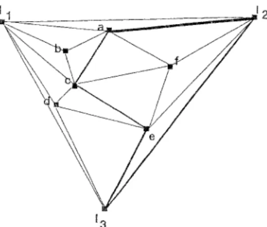
Miller (1986) assumed that we were given a planar graph G with nonnegative weights assigned to vertices, faces, and edges which sum to 1. For o u r case, we simply assume that the weights of faces and edges are all zeros. In other words. weights are assigned o n l y to vertices. For a simple cycle B of G, the size of this cycle is the number of the vertices on B. Note that a simple cycle of G will always divide G into two parts, the interior A and the exterior C. The weight of the interior part (resp. the exterior part) is the sum of weights of vertices in the interior part (resp. the exterior part). Figure 2.1 shows a planar graph and the thick edges form a simple cycle. F o r this case, the size of the cycle, the weight of its interior, and the weight of its exterior are 7, 0.35, and 0.45, respectively.

The theorem proved by Miller (1986) is now stated as follows. (Note that it is slightly different from that original one stated by Miller (1986)0 because we do not assign weights to faces and edges.)

0.05

_0.0.5

0.02 ~

0.05

C O.Ot

O.

0.05

THEOREM 2.1 (Miller, 1986). I f G is a 2-connected planar graph with all nonnegative weights assigned to vertices which sum to 1, there exists a simple cycle, called the simple cycle separator, of size at most 2 ~ , dividing the graph into interior and exterior two parts, such that the sum of the weights in both parts is no more than two-thirds, where d is the maximum face size (the face size is the number of edges contained in the facial cycle) and k is the number of vertices in G.

In our case we are interested in the maximal planar graph (Nishizeki and Chiba, 1988), where d is equal to 3. Hence the size of the separator is accordingly x / ~ .

Given a set S of P unfixed supply points, the Delaunay triangulation of S cannot be a maximal planar graph, because the outer face is not necessarily of size 3. There is a simple way to change the Delaunay triangulation graph into a maximal planar graph, by adding a set I of three extra points to form a triangle enclosing all points in S. Let S' = S w I. The Delaunay triangulation of S' is a maximal planar graph, because its outer face contains exactly three edges and other faces are triangulated. Hence we can apply Theorem 2.1 to the Delaunay triangulation of S'.

In our algorithm we treat the three points of the triangle as supply points, and they are not related to any demand point. We define the enclosing I as follows: the enclosing points are three points which form a triangular boundary enclosing all points, such that no demand point's distance to its closest supply point is longer than its distance to any of the enclosing points. We can see that it is trivial to find these enclosing points. We simply select them far enough from any of the demand points.

By applying Theorem 2.1 to S', we can see that there exists a simple cycle separator B with size less than x f ~ + 3) which divides the Delaunay triangula- tion graph of S' into the interior and exterior parts, such that the number of unfixed supply points in each part is less than 2P/3. This result is derived by assigning zero weights to the enclosing points and equal weights to the unfixed supply points.

Nevertheless, Miller's simple cycle separator theorem cannot guarantee that the sets of D and S divided by the simple cycle separator satisfy the third property of the B-cycle. This is due to the fact that we construct our Delaunay triangulation graph out of the unfixed supply points in S only and totally ignore the demand points in D. In Figure 2.2 we show an example. In this example, there exists a

C "

" ~ ~"v-~" Its nearest supply point

"/.~" isinAs

A V o r o simple cycle separator

404 R.Z. Hwang, R. C. Chang, and R. C. T. Lee demand point lying in Cd and its closest supply point is in A,, if we treat the simple cycle separator as the desired B-cycle.

In the following we define the rules which construct the B-cycle from the smaple cycle separator B. Let Vor(S') denote the Voronoi diagram of S' (Voronoi, 1907; Preparata and Shamos, 1985; Edelsbrunner, 1987~ and let DT(S'~ denote the Delaunay triangulation of S' (Delaunay, 1934; Preparata and Shamos. 1985; Edelsbrunner, 1987). Given a simple cycle separator B on DT{S'), the correspond- ing B-cycle is defined as follows: for every connected pair of supply points s~ and sj in the simple cycle separator B, find its associated edge e in the Vor(S'). (Note that for any edge on the DT(S'), there is an associated edge on Vor(S').) Let one of the two points of the edge e be v~j. Draw sivlj and vi~sj. This new corresponding cycle, consisting of all such siv~fs and viisj's, is called the B-cycle of S'.

Consider Figure 2.3. Figure 2.3(a) shows a simple cycle separator and Figure 2.3(b) shows the corresponding B-cycle.

It is obvious that the B-cycle, constructed by the above rules, satisfies the first property, that is, the number of unfixed supply points in the B-cycle is less than

,,/8"(P + 3). Now we want to show the second property. From Miller's simple

cycle separator, we know that the sets of unfixed supply points divided bv the simple cycle separator satisfy the second property. Now we want to show. in the following lemma, that the sets of unfixed supply points divided by a simple cycle separator B are identical to that divided by its corresponding B-cycle. Yhis way we can prove the second property.

LEMMA 2.1. The sets of unfixed supply points in the interior and exterior parrs partitioned by the simple separator cycle B and its corresponding B-cycle are identical.

(a)

Fig. 2.3. (a) A simple cycle separator and (b)

. / !

\

Fig. 2.4. No unfixed supply point in the shaded area.

PROOF. Consider any edge sisi in the separator cycle B. Let e be the Voronoi edge associated with sisj. Let vq be one of the vertices on e. Consider si, si, and v~j, as shown in Figure 2.4. According to Theorem 5.8 of Preparata and Shamos (1985), there is no unfixed supply point in this triangle. Therefore, if we replace

sls~ by s~vij and v~jsi, the partition of unfixed supply points is not changed. []

The last and most important property is the third one. Now we want to show that, for each demand point in Ae (resp. Cd), its nearest supply point is in A~ (resp.

Cs) or B~ u [3.

THEOREM 2.2. Given an instance of GDEPM(P, D, [3) or GDEPC(P, D, [3), its optimal solution S, and the corresponding B-cycle, let B~ be the set of supply points on the B-cycle. The B-cycle divides D (resp. S) into interior and exterior two parts, called Ad and C~ (resp. A~ and C~). Then, for each demand point in A a (resp. Ca), its nearest supply point is in A~ (resp. C~) or B~ ~ ft.

PROOF. To show that, for each demand point in Aa (resp. Cd), its nearest supply point belongs to A~ (resp. C~) or fl ~ B~, we first use the fact that no edge in the B-cycle crosses V(s') where s'~B~ (where V(s) denotes the Voronoi polygon associated with s, s e S). This fact is due to the rules constructing the B-cycle.

Let d ~ A d and let the nearest supply point Of d be s e C~. Hence d must be on

V(s), if Vor(S w I) is constructed, where 1 is the set of enclosing points. Because d

is in the interior part of the B-cycle and s is in the exterior part, there must exist some edges of the B-cycle passing through V(s). However, from the above fact of the B-cycle, the edges can only cross the polygon associated with the unfixed supply points in B~. Therefore no such a demand point d exists. This means that the nearest supply point of any demand point in A d (resp. Ce) must be in A~ (resp.

C~) or B~ u fi. []

The above theorem certifies that the two subproblems are independent. This independent property is very important because it guarantees the correctness of our searching over separators approach.

Now let us show a simple example to explain how to divide the input points by using the B-cycle. In this example we assume that S' is given as in Figure 2.5 and P is 18. The largest size of the B-cycle is therefore at most ,,/8 "(18 + 3). In

406 R.Z. Hwang, R. C. Chang, and R, C. T. Lee

L.

9 I I | 0 i i

.r

/ B m o r n i i =o. ~ . \ " . " / /

"

/

/

Fig. 2.5. An example of how to divide input points by using a B-cycle. n, demand points; O, supply points.

Figure 2.5 there are a set of demand points (denoted as squares), a set of unfixed supply points (drawn as dots), the enclosing points, and the B-cycle of the Delaunay triangulation of

S',

constructed out of two enclosing points and four unfixed supply points. The B-cycle divides the points into two parts. We can see that, for each demand point in the interior (resp. exterior) part of the B-cycle, its nearest supply point is either in the interior (resp. exterior) or on the B-cycle.

2.3. Generating Possible B-Cycles.

In the preceding subsection we showed the properties and the existence of a B-cycle. In this section we introduce two procedures, which will generate possible B-cycles, one of which is the desired B-cycle.

Let us first discuss the problem of generating a simple cycle separator. A simple cycle separator consists of less than ~ + 3) points. We exhaustively try all possible ways of selecting i points out of n + 3 points (including the three enclosing points), where i ranges from 3 to ,fi(-P + 3) (for a simple cycle needs at least three

points). (Thus, there are at most

ways to select i points.) For each set of i points, we construct a complete graph. Out of this complete graph, we select any i edges and test whether they form a simple cycle or not. (Since there are i" (i - 1) edges in the graph, there are at most 0 possible selections. To test whether they form a simple cycle needs

l

at most 0(i2).) One of these cycles must be the desired simple cycle separator. From the above discussion, we know that the time needed to generate all possible simple cycle separators is

O ( ( ( n + 3 )

~ . ~ ( i . ( i - - 1 ) ) . i 2 ) = O ( n C l . j ~ + c 2 ) ,

\ \ ~ / 8 ( P + 3)/ k i

where c 1 and C 2 are some constants.

Next, we should try to construct the corresponding B-cycle of a given simple cycle separator by using the rules defined in Section 2.2. Those rules tell us that we can construct the B-cycle by connecting all such

slviSs

and

vijsj's

for each edge

s~sj

in the simple cycle, where vlj is the Voronoi polygon shared by

V(si)

and

V(sj),

where

V(si)

(resp.

V(sj))

is the Voronoi polygon associated with si (resp. st). We cannot find vii directly, for

V(sl)

and

V(sj)

are unknown. Therefore we propose an exhaustive search approach to find all possible candidates of vii. The Voronoi vertex vij must be the center of the circle formed by s~, sj and the third unknown point

Sk.

We know that

Sk ~ S w I.

Therefore

Sk ~ D u I.

We may try all points in D ~ I as the candidates of

Sk.

This way, for each edge

sis~

in the simple cycle, we have ID u I[ = (n + 3) possible viSs, by finding the center of the circumscribed circles defined by the three points s i, s j, and any point in D ~ I.

Consider the time complexity of the above steps. Step 1 takes

( ~ + 3 ) " ( i + 1 ) ! < ( n + 3 ) i + 1 + 1

steps. Steps 2-8 take O(i 2) time. The time needed in this procedure is

O((n + 3) '+ 1. i2).

Since i + 1 is the number of points in the simple cycle and (i + 1) < x / ~ + 3), we can see that the time complexity is bounded by

O(nC3"/g+c4),

where c 3 and c 4 are some constants.

In the next section we show the entire algorithm to solve the G D E P M problem, by using the above two procedures.

408 R.Z. Hwang, R. C. Chang, and R: C. T. Lee

2.4. The Algorithm and Its Time Complexity~

In this section we present an algorithm to solve the G D E P M problem. This algorithm is called Algorithm G D E P M .

Algorithm G D E P M ( P , D,/3, S, C). (An algorithm ro solve the G D E P M problem based upon the search over separators strategy.)

Input:

D, a set of n demand points;/~, a set of fixed supply points; and P; a number.

Output:

S, a set of supply points which is an optimal solution to the G D E P M prob!em; C, the optimal cost of the G D E P M problem. Step 1. Step 2. Step 3. Step 4. Step 5. Step 6. Step 7. Step 8. Step 9. Step 10. Step 11. Step 12. Step 13. Let C = oo. If P _< 3, then do steps 3 5'

F o r each subset S' c D of P points do:

For all points in D, find their corresponding nearest points in

S' w ~

and sum up all these weighted distances to C'. I f C > C ' , t h e n C = C ' a n d S - S ' .

Else do steps %13:

Generate all possible B-cycles (using the m e t h o d discussed in the above section).

F o r each possible B-cycle, we divide D into the interior part A} and the exterior part C5, and do steps 9-13:

F o r k = 0 to

2P/3

do: I f ( P -

i - k) <_ 2P/3

do: Call G D E P M ( k , AS, B'~ ,~/3, S~, C 0. Call G D E P M ( P ~ i - k, C5, B; ~/3, $2, C2). I f C t + C 2 < C , t h e n S - S ~ w S 2,~B'~and C = C 1 - ~ C 2 .

N o w let us discuss the time complexity of Algorithm G D E P M . Let the total time complexity of this algorithm be

T(P).

We can see that steps 2-5 take

O(n e+l

.P), P < 3. Step 7 needs O(n ~c',/g+~)+(c3"j~+c4)) =

O(nC~/g+c6),

as described in the above section, where c 5 = c 1 + c 3 and c 6 = c 2 -,- c,~. Steps 9-13 are bounded by

0((2P/3).

2. T(2P/3)) _<

O(2n. T(2P/3)),

for P _< n. Therefore the time complex- ity from step 7 to step 13 is bounded by

O(n c~,/g+c~ 1). T(2P/3).

Hence we have the following formula:

{<O(n~,/g+~+l).T(2P/3)

when P > 3.

T(P)

O(ne+ 1. p) ~

O(n 4) when P < 3.

When P > 3,

T(P) < O(n c~'/g+~+

t).

T(2P/3)

< O(n~,,pf+ ~ + ~). O(n~,,~2/Y~ + c~ + 1). T(4P/9))

' + t ) " |og3/2 P )

< O(n~S(,/p + ,/2e/3 + ,/4e/9 -..) + (c6 +

< O(nCS.(1/(1-,j~/3)).,~-+lc6+l)-log3/2e) = O(rlO(,/Pl).

2.5. The Discrete Euclidean P-Center Problem. After showing how the D E P M problem can be solved by the searching over separators strategy, in this section we show that the D E P C problem can be solved in exactly the same way.

The D E P C problem is defined as follows: given a set D

= {dl, d2,... ,dn}

of demand points, find a set S of P supply points from D, in order to minimize

Megiddo and Supowit (1984) proved that the E P C problem is NP-hard. Drezner proposed an O(n 2v+ 1 "log n) algorithm (Drezner, 1984) for the E P C problem, which can be improved to O(n 2v-~.log n) by combining it with the result that the Euclidean 1-center problem can be solved in O(n) time (Megiddo, 1983). The way of combining these two results is similar to that of Drezner (1987).

We can see that the D E P C problem is almost exactly the same as the D E P M problem. We need to define a 9eneralized discrete Euclidean P-center problem as follows: given a set D of n demand points, a set/~ c D of fixed supply points, and a number P, select a set S of P supply points from D where fl and S are disjoint, such that

is minimized.

We may denote the above problem as the GDEPC-(P, D,/~) problem or the G D E P C problem. Thus, if we change step 13 of algorithm D E P M to be as follows:

Step 13. If max{C1, Cz} < C, then S = S 1 u S 2 t j B s and C = max{C1, C2}.

then algorithm D E P M can also be used to solve the D E P C problem with time complexity O(n~

3. The Euclidean P-Center Problem

3.1. Drezner's Algorithm. The E P C problem is similar to the D E P C problem,

except in this case the supply points do not have to be chosen from demand points. Yet, by using Drezner's algorithm (Drezner, 1984), we can easily transfer this problem to a problem similar to the D E P C problem and thus the search over

separators strategy can be used again.

Note that P circles of radius r can cover n demand points if and only if there are P supply points and the longest distance between each demand point and its closest supply points is r. Drezner (1984) pointed out that a circle is defined by one, two, or three points. F o r the case of circles defined by three points, these three points define the boundary of the smallest circle enclosing all three of them.

410 R.Z. Hwang~ R. C. Chang, and R C. Y. Lee F o r the case defined by two points, they f o r m the diameter of this circte. A circle defined by only one point is a degenerated case, where the radius of this circle can be considered as zero and the entire circle contracts to one point. Hence, we ( ~ ) ( n ) and ( ~ ) circles defined can simply e n u m e r a t e all of the circles. There are ' 2 '

by one, two. a n d three points, respectively. We call these circles the bounding circles.

Given a n y solution to the P-center problem, the largest radius r (the longest of all distances between each d e m a n d point and its closest supply point) must be equal to the radius of one of the b o u n d i n g circles b o u n d e d by two or three points. Hence, if we have an algorithm which can determine whether P circles o f a given radius r can cover all these points, we can perform a binary search over all radii of the b o u n d i n g circles to find an optimal one.

Let us sort all of the radii of the b o u n d i n g circles. Then we choose one of them, say r, a n d we ask the following question: can P circles of radius r cover the n points? To answer this question, a p p a r e n t l y we have to determine where these P circles should be placed.

D r e z n e r (1984) also showed that there are only

O(n 2)

possible supply points for a given radius r. He claimed that there exists a set Sp of O(n 2) possible supply points, such that if P circles of radius r can cover the n d e m a n d points, then we can find P circles centered at some of the points in Sp which can cover the n d e m a n d points. The points in set Sp are called the possible supply points, found as follows: F o r a n y two points in the n d e m a n d points, we find the two circles of radius r passing t h r o u g h these two points. The set Sp is the union of the centers of these circles and the n d e m a n d points.

N o w let us see w h y Drezner's claim holds. Assume that we have found that a set C = {cl, c2 . . . Ce} of circles of radius r can cover all n d e m a n d points. If there are m o r e than two d e m a n d points o n the b o u n d a r y of circle ci ~ C, then the center of ci belongs to Sp. If there are less than two d e m a n d points on the b o u n d a r y of circle cj ~ C, then there are two possibilities. O n e is that this circle covers only one d e m a n d point. In this case we m o v e this circle so that it centers at this d e m a n d point. A n o t h e r case is that this circle covers m o r e than two d e m a n d points. In this case we can m o v e this circle until two d e m a n d points touch the b o u n d a r y of this circle. Again this new center belongs to Sp. We can see that these new circles cover the same set of d e m a n d points as the old circles do. So we have a new solution and the centers of the circles in this solution are all points in Sp.

Therefore we can select any P points in Sp a n d then check whether these circles of radius r centered at these P points cover all of the n d e m a n d points. Since there are O(n 2) possible supply points, we have (,O 2) possible selections, and it takes

O(n) time to check whether these P circles cover all points, a n d O(log n 3) = O(log n)

to do the binary search~ So the time complexity is O(n 2e + 1. log hi.

3.2. The Searehin9 over Separators Strategy To Solve the (P, D, Sp) Circle Cover

Optimization Problem, As we discussed above, o u r basic problem is as follows:

points (generated by using Drezner's algorithm (Drezner, 1984)), determine whether there exists a set S c Sp of P supply points, such that the P circles of radius r centered at these P points can cover the n demand points. We call this problem

the

(P,

D, r, Sp) circle cover decision problem

(the (P, D, r, Sp) CCD problem).

In order to solve the above (P, D, r, Sv) CCD problem, we may first solve the following

(P, D, Sp) circle cover optimization problem

(the

(P, D, Sp)

CCO problem): given a set D of n demand points and a set Sp of

O(n 2)

possible supply points, find the smallest

rs,

such that P circles of radius rs centered at some P points selected from Sp can cover the n demand points. We can see that if this r S is longer than r, then the answer to the

(P, D, r, Sp)

CCD problem is "false"; otherwise it is "true." Thus, if the

(P, D, Sv)

CCO problem is solved, the (P, D, r, Sv) CCD problem is also solved.

It can be easily seen that the (P, D, Sp) CCO problem is similar to the GDEPC-(P, D, fl) problem except in this case there are O(n 2) points in Sv and we select the supply points from

Sp,

instead of D. Thus the algorithm for solving the G D E P C problem can be used to solve the

(P, D, Sp)

CCO problem with time complexity

O(n~

4. The Euclidean Traveling Salesperson Problem

4.1. Preliminaries.

In the above sections we described how to apply the searching over separators strategy to the D E P C problem. We now show how the searching over separators strategy can be applied to solve

the Euclidean traveling salesperson

(ETSP) problem.

In this problem, given n points in the plane, we are asked to find a shortest cycle out of these n points. This problem is an NP-hard problem (Papadimitriou, 1977; Papadimitriou and Steiglitz, 1976) and it can be solved by the dynamic programing strategy in time O(2"n 2) (Held and Karp, 1962; Horowitz and Sahni, 1978; LaMer

et al.,

1985). A very thorough review of many algorithms for this problem can be found in Lawler

et al.

(1985). We show that through the searching over separators strategy, we can obtain an algorithm for the ETSP problem with

O(n ~

time.

4.2. The Generalized Euclidean Traveling Salesperson Problem.

As we did in solving the D E P M problem, we first generalize our ETSP problem into the following: Given a set V = {vl, Va,..., v,} of points and a set

T = {(t,, tl),(t2, t~), ...,(t~, t~)}

of

terminal pairs,

we want to find a set of m paths, satisfying the following conditions:

(1) Every path starts from ti and returns to t'i, where 1 <_ i < m. (2) Every point in V is included in exactly one of these paths. (3) The total length of these paths is minimized.

412 R.Z. Hwang, R. C. Chang, and R. C. T. Lee

e

Fig. 4.1. An optimal solution to the ETSP problem.

We m a y call the generalized Euclidean traveling salesperson problem ! the G E T S P problem) with such V a n d T as inputs the (V. T~-GETSP problem, W h e n V = {v2, v3, ..., v,} and T = {(v~, Vl)}, this G E T S P p r o b l e m is degenerated to the E T S P p r o b l e m with v 1 .. . . . v, as inputs. Again, for reasons which will become clear later, we try to solve the G E T S P problem.

Let us imagine t h a t given an E T S P p r o b l e m with a set V of n points as input a n d we have an optimal solution to this problem. We first show that, based u p o n the optimal solution, we can find a cycle separator properly dividing the input sets V into two parts of inputs V~, T~ and V~, T~ of the G E T S P problems such that. if we solve the two G E T S P problems a n d then merge the solutions, we can obtain an optimal solution of the original one.

Consider Figure 4.1, which shows a set of points a n d an optimal solution to the E T S P problem. We then add a set I = {I~, 12, 13} of three enclosing points

which inscribe all points m V, and construct a triangulation o u t of the points in V u I where every edge in the optimal solution is also an edge in this triangulation. Since this triangulation is a maximal planar graph, let the points in I be zero weighted vertices a n d lel the others be equal weighted vertices. Then from Miller's simple cycle separator t h e o r e m (Miller, 19861, there exists a simple cycle separator which divides the points in V into the interior part V~ and the exterior part V~, respectively, such that there are no more t h a n ,,/8" {n -,- 3t vertices in the simple cycle separator, [Vaj < 2n/3 and ]V~ _< 2n/3, where n is the n u m b e r of points in v and in this case n = 6. Here the three input points, namely, a, c, and e are on the simple cycle separator, as shown in Figure 4.2. T h u s we n o w have two G E T S P problems, defined as follows:

(1) The interior s u b p r o b l e m with V~ = {f}, T, = {(e, a)} as inputs. (2) The exterior s u b p r o b l e m with V~ = {b, d}, T~ = {(a, c), tc, e)} as inputs.

After solving the above two G E T S P problems, we obtain the three paths. Pl = (a, b, c), P2 - (c, d, el, and P3 = (e, f, a). Using a simple m e r g m g process, we can derive the original optimal solution p - (a, b, c, d, e, f, m.

The above example shows h o w to divide the E T S P problem into two G E T S P problems. F o r solving the subproblems, we would recursively divide these G E T S P problems. It is n o t difficult to see that the G E T S P problem can also be divided by the same principle, except that there is an extra input data T In this new dividing process, we construct the triangulation out of the points in V, 1. a n d T. Also let the points in I be zero weighted vertices and let the others be equal

I I I 2

[3

Fig. 4.2. A simple cycle separator showing the three input points a, c, and e.

weighted vertices. Then, from Miller's simple cycle separator theorem (Miller, 1986), there exists a simple cycle which divides the points in V and T into the interior parts V,, T'a and the exterior parts V~, T'c, respectively, such that there are no more than x/8. (n + 2m + 3) vertices in the simple cycle and I V,t + I Z'a] <-

2(n + 2m)/3, I V~I + I T;] -< 2(n + 2m)/3, where 2m is the number of points in T. In the following we present a dividing process, which would decompose a (V, T)-GETSP problem into two subproblems. We later show that if we solve these two subproblems and then merge the two solutions, we would obtain an optimal solution to the original (V, T)-GETSP problem. As explained later, to execute this dividing process we must have an optimal solution to the (V, T)-GETSP problem.

A Process To Divide a (V, T)-GETSP Problem into Two Subprobiems

Input: A (K T)-GETSP problem, where V = {Vx, U 2 , . . . ,

Vn}

and T =

{(tl, t]), (t 2, t~) . . . (tin, t;,)}, and an optimal solution to this problem, namely, a set S of m paths Pl, P2,..., Pro"

Output: Two subproblems: the (V~, Tb)-GETSP problem and the (V~, T~)-

GETSP problem, such that the merging of the solutions to the above two problems will result in an optimal solution to the (V, T)-GETSP problem.

Step 1. Find the set I = {I 1, 12, I3} of three points which inscribes all points in V and T.

Step 2. Construct a triangulation graph out of these points in V, T, and I, such that each edge in the optimal solution is an edge in this triangulation.

Step 3. Let the weights of points in I be zero and let others be any nonzero constant. Use a simple cycle separator B to divide V (resp. the points in T) into the interior part V~ (resp. T'a) and the exterior part V~ (resp. T;). Lct Vb be the points on the simple cycle separator B which belong to V.

414 R.Z. Hwang, R. C. Chang, and R. C. T. Lee

Step 4. Let T~ = T~ = ~ . Step 5. F o r i = 1 to rn do: Step 6. Call Procedure

DIVIDE_TERMINAL(pl, V,, V~, T;, T;, Vb, T~, T~). Step 7. T, = T~ w r / , T~ = T~ tj T~.

Step 8. Output two subproblems: the (V~, T~)-GETSP problem and the (V~, T~)-GETSP problem.

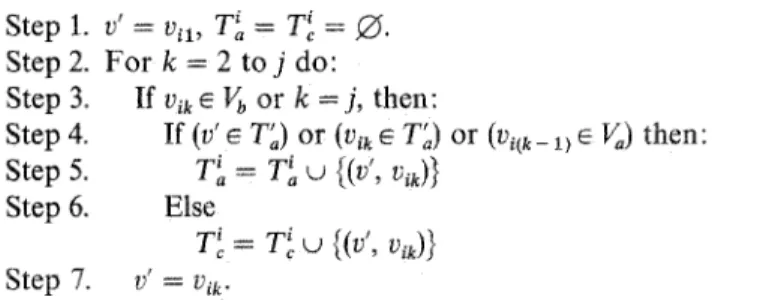
In the above process the critical procedure is Procedure D I V I D E T E R M I N A L . This is a linear scan procedure, which scans the points along a path. If the point being scanned is a point in the simple cycle separator, then some appropriate action is taken. This procedure is now described:

Procedure DIVIDE TERMINAL(pl, V~, Vc, T;, T;, Vb, T~, F~)

I n p u t : A path Pi = (vii, vi2 . . . vii), V,, V~, T'a, T'~, and Vb.

O u t p u t : r~, and Tic where r / and T~ are both sets of terminal pairs. Step 1. v' = v a , Ti~ = T~ = ~ .

Step 2. F o r k = 2 to j do: Step 3, If vik e Vb or k = j, then:

Step 4. If (v' ~ T~) o r (l)ik e r'~) o r (1)i( k_ 1) ~ Va) then: Step 5. T / = T~ u {(v', vik)}

Step 6. Else

= u

Step 7. v' = vik.

In the following we show an example to illustrate how Procedure D I V I D E - T E R M I N A L works. Consider Figure 4.3. We have a path Pi = (a, b, c, d, e, f , g, h),

where a, h e T'c, b, e, g e Vb, c, d e V~, and f ~ V~. Applying the above procedure. we obtain T~ = {(a, b), (e, g), (9, h)} and T~ = {(b, e)}. We now show that after we solve the two subproblems, we can merge the two solutions and obtain an optimal solution to the original problem.

Note that in the dividing process, Procedure D I V I D E _ T E R M I N A L sequenti- ally divides a path into sets of terminal points. Thus, for path Pi, let us assume that the terminal pairs resulting in both interior and exterior parts from applying the above procedure a r e (til , t'il), (ti2 , t'i2) . . . (t~j, tlj), where ril and t~j a r e the

starting and terminating points ofpi, respectively. After solving the (Va, T,)-GETSP

El a a simple cycle separator

, " Z V

f

problem and the (V~, T~)-GETSP problem, til is connected to th through a path, t~2 is connected to t'~2 through a path, and so on. Moreover, ti~, which is a starting point of p~, is connected to t',j, which is a terminating point of pi. In other words, after solving the (V~, Ta)-GETSP problem and the (V~, T~)-GETSP problem, we have p'~, p~, p ; , . . . , p" in which the starting point and terminating point of P'i are the same as those of p~ of the optimal solution to the (V, T)-GETSP problem. We may conclude that after solving the (V,, T,)-GETSP problem and the (V~, T~)- GETSP problem, we have obtained a solution to the (K T)-GETSP problem. We now prove that this solution is an optimal solution.

Let S, and Sc denote optimal solutions to the (V~, T~)-GETSP problem and the (V~, T~)-GETSP problem, respectively. Let S denote an optimal solution to the (V, T)-GETSP problem, and let COST(S) denote the cost of solution S. We show that COST(S,)+ COST(S~)= COST(S). Assume otherwise. Then there are two cases:

Case 1." COST(S,) + COST(So) < COST(S). This is impossible because COST(S) is the cost of an optimal solution to the (V, T)-GETSP problem.

Case 2: COST(S,) + COST(S~) > COST(S). Let us decompose the optimal solu- tion into two parts, one relating to points in the (V~, T~)-GETSP problem, denoted as S'a, and the other relating to points in the (V~, T~)-GETSP problem, denoted as S;. Then COST(S) = COST(S;) + COST(S;). In other words, we have

COST(S,) + COST(So) > COST(S;) + COST(S;).

Without loss of generality, we may assume that COST(S~) > COST(S'a). Again, this is impossible because COST(S,) corresponds to the cost of an optimal solution to the (V,, T,)-GETSP problem.

In conclusion, we have the following lemma:

LEMMA 4.1. Let S, and Sc denote the costs of optimal solutions to the (V,, T~)- GETSP problem and (V~, T~)-GETSP problem, respectively, and let S denote an optimal solution to the (V, T)-GETSP problem. Then

COST(S) = COST(Sa) + COST(So).

There is still one problem which we have to solve. Note that after solving two (V, T)-GETSP problems, we get a set of paths. These paths cannot intersect with one another because Miller's theorem can only be applied to the planar graph. It is obvious that there is no intersection in the optimal solution to the ETSP problem. Assume that S is an optimal solution to some ETSP problem, vlv2 and v3v 4 are in S, and they intersect each other, then we can draw vlv3, VzV, ~ or VxV4, v2v 3 instead of VlV 2, v3v4 in S. Both will derive a lower cost than the original one and one of them must be a legal solution. So we have another legal solution with lower cost than S. Therefore any cycle with intersections must not be an optimal solution to the ETSP problem.

We next show that if the initial problem is an ETSP problem~ then at each stage after solving two GETSP problems, the resulting paths do not intersect and

416 R.Z. Hwang, R. C. Chang, and I~ C. T. Lee

Miller's t h e o r e m can always be applied. Assume otherwise. At a certain stage, two paths intersect after solving two G E T S P problems. T h e n after we merge these paths b a c k recursively, we finally obtain a cycle with intersections. This is impossible because o u r initial p r o b l e m is an E T S P p r o b l e m , and its solution should be a cycle without intersections.

4.3. Generating A l l Possible I n p u t Instances. N o t e that the a b o v e discussion is based u p o n an a s s u m p t i o n that an o p t i m a l solution is available to us. O f course, we do not k n o w a n y o p t i m a l solution in advance. Therefore o u r strategy is to generate all possible simple cycle separators, a n d then we find the best result with respect to each possible simple cycle separator. Because the largest size of a simple cycle s e p a r a t o r is , j ~ n + 2m - 3), we m a y select i edges, where 3 < i <_ ,,/8 "(n - 2m + 3), f r o m the complete g r a p h constructed f r o m the points in V, T, a n d I. If these i edges form a simple cycle without a n y intersection then test whether this cycle can divide the rest of the points in V. T i n t o V~, T ; and V~,

T;, such that I V~ u T',] _< 2(n + 2m)/3 and I V~ u r ; l _< 2(n - 2m)/3. If this cycle satisfies the a b o v e conditions, this is a candidate of the simple cycle separator. Since we exhaustively generate all possible such simple cycles, the one which derives the best result must be the desired one. T h e following is o u r a l g o r i t h m to generate all these possible simple cycle separators.

Procedure G E N _ C Y C L E S _ B I V, T, B')

F u n c t i o n : G e n e r a t e a set B ' of simple cycles of which one is the simple cycle s e p a r a t o r on the maxima] p l a n a r g r a p h from the points in F. T, and 1, and the edges in the p a t h s of an o p t i m a l solution.

I n p u t : A set V and T.

Output." A set B' of simple cycles.

S t e p l . L e t B ' - ~ a n d l e t T r be the set of points m T. S t e p 2 . F o r i - 3 t o ~ / 8 ( [ V : [ T ' l + 3 ) do:

Step 3. Find B'~ = {b'slb'~ ~ [ V w T' ~J 1) a n d Ib's - i}. Step 4. F o r each b'~ s B's do:

Step 5. C o n s t r u c t the complete g r a p h out of the points in b's. Step 6. F o r each subset of i edges in G do:

Step 7. If these i edges c a n n o t form a simple cycle, then j u m p to step 6 and try the next instance: else denote this simple cycle as b.

Step 8. If there exists a n y intersection in b, then j u m p to step 6 and try the next instance.

Step 9. Use b to divide the points in V and T into interior parts V,, T'a and the exterior parts t~, T'c. (Apply the point !ocation algorithm of P r e p a r a t a and S h a m o s (1985).) If [I ga u r ' a > 2(n ~ 2m)/3)or([ V~ ,~ T'r > 2(n ~ 2m)/3), then j u m p to step 6 and try the next instance.

Step 10. B' := B' ~ b. Step 11. Return B'.

e

c

U

D

l

f

a

~

b g

[]

Fig. 4.4. Two terminal pairs, (a, b) and (c, d), and three points,

e,f,

and 9, on the simple cycle separator.

This procedure is slightly modified from Procedure G E N _ C Y C L E S _ A discussed in the preceding sections. By using a similar method, we can prove that the time complexity and the number of cycles are both bounded by

O((n +

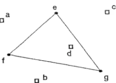
2m) c~ (,/~ + 2m)+ cb), where c a and c b are some constants.

In this procedure we show that we can find all possible simple cycle separators. We still have to face one problem. We have to decide all of the terminal pairs. For instance, in the example illustrating the dividing procedure, we generate two sets of terminal pairs T~ = {(a, b), (e, 9), (9, h)} and Ti, = {(b, e)}. Since no optimal solution is available to us, how can we determine these two sets?

Let us consider Figure 4.4. In Figure 4.4 there are two terminal pairs (a, b) and (c, d). The points on the simple cycle separator are e, f, and 9. Of course, there are many other points which are neither terminal points nor points on the simple cycle separator. F r o m Procedure D I V I D E T E R M I N A L , it can be seen that points which are neither old terminal points nor points on the simple cycle separator are irrelevant to our dividing process. Therefore, in the following, we only consider points which are originally terminal points or points on the simple cycle separator.

Suppose that we are given two terminal pairs (a, b) and (c, d). We are also given points on the simple cycle separator e, f, and 9. There are many ways of forming paths by using these points. Our job means to assign e, f, and 9 to either (a, b) or

(c,d)

such that two paths will be formed: one connecting a to b and the other connecting c to d. In the following we list some of them:

(1) (a,e,b) and ( c , f , g , d ) (2) (a, e, b) and (c, 9, f, d) (3) (a, b) and (c, e, f, ~, d) (4) (a, b) and (c, f, e, g, d) (5)

(a,f,g,b)

and (c, e, d) (6) (a, g,f, b) and (c, e, d) and so on.

It can be seen that in each case we assign a subset of e, f, and g to (a, b) and the rest of the points to (c, d). Note that the subset can be an empty set. Moreover, after a subset of points from e, f, and g are assigned, they can be permuted.

418 R.Z. Hwang, R. C. Chang, and R. C. T. Lee the following we list some of them:

(1) (a, e, b) --* (a, el, (e, b)

(c, f, g, d) ~ (c, f), (f, g), (g, d)

(2) (a, e, b) ~ (a, el, (e, b)

(c, g, f, d) --+ (c, g), (g, f), (f, d) (3) (a,b) ~ (a, b) (c, e, f, g, d) --, (c, el, (e, f), (f, 9), (9, d) (4) (a,b) -+ (a, b) (c, f, e, g, d) --+ (c, f), (f, el, (e, 91, (g, d) (5) (a, f, g, b) ~ (a, f), (f, g), (9, b) (c, e, d) --* /c, e), (e, d) (6) (a, g,f, b) -, (a, g), (g, f), (f, b) (c, e, d) -, ~c, el, le, d)

F o r each terminal pair, we assign it to interior or exterior. For instance, consider (a, el. Since a is an exterior point, (a, et is an exterior terminal pair. On the other

hand, (g, d) is an interior terminal pair. because d is an interior point. For (f, g),

it can be assigned to either exterior or interior. Therefore. given the set of terminal

pairs {(a, el. (e, b), (c, f), (f, g), (g, d)}, we can generate the following possible

terminal pairs of the snbproblems:

(1) The interior terminal pairs: {(c, f), (f, g)}. The exterior terminal pairs: {(a, el, re,

b), (g, d)}.

(2) The interior terminal pairs: {c, f)}.

The exterior terminal pairs: {(a, el, (e, b), (J; g), (g, d)}.

We now list the basic steps to generate all the new terminal pairs. We are given the original terminals (tl, t'l), (t2, @, .... (tin, t;,) and the set of nonterminal points in the simple cycle separator {bl, b2 . . . bk}. Our first step is to generate all possible permutations of {bl, b2 . . . bk}. For instance, for the above example, we have (e, f, g) ~e, g, f ) (g, e, f ) (g, f, e) (f, g, e)

(L e, 0)

Since there are two original terminal pairs, for each permutation, we view it as a sequence and generate all possible two continuous subsequences. For example,

consider

(e, f, g).

There are four possible ways to partition it into two subsequences:

( ) (e,f,g)

(el (f, g) (e, f ) (g)

Each subsequence can be partitioned in this way. After all sequences are parti- tioned, we assign the first subsequence to (a, b) and the second subsequence to (c, d). Thus from the above pairs of subsequences, we have the following paths:

(a,b) (c,e,f,g,d)

(a,e,b)

(c,f,g,d)

(a,e,f,b)

(c,g,d)

(a,e,f,g,b)

(c,d)

It may be wondered why (c, e, d), for instance, is not generated. This will be generated later by applying the procedure to the sequence (f, 9, e). (f, 9, e) can be partitioned into (f, 9) and (e). This will produce the path (c, e, d).

After generating paths, we then scan each path linearly and produce terminal pairs. For instance, for (a, e, b), we have (a, e) and (e, b) as terminal pairs.

Note that given a simple cycle separator, the sets V,, V~ of nonterminal points of the inputs of the subproblems are all the same. The following procedure is our detailed algorithm to generate all possible input instances of the subproblems:

Procedure GEN_INPUTS(V, T, b, p)

Input:

V = {vi, v2 . . . v,}, a set of points;

T = {(t l, t'i), (t2, t~), ..., (tin, t~,)}, a set of terminal pairs; and b, a simple cycle which goes through some points in V, T, and I.

Output:

p = {(Va, V~, Ta, T~)I(V,, T~), (V~, T~) are the candidates of the

input instances of the interior and exterior subproblems, respectively.}

S t e p l . p = ~ .

Step 2. Use the simple cycle b to divide the points in V and T into the

interior part

V,, T'a

and the exterior parts V~, T;, respectively.

(Apply the point location algorithm of Preparata and Shamos (1985).) Let Vb be the nonterminal points of Vin the simple cycle. Step 3. Generate all permutations of points in Vb.

Step 4. For each permutation q' = (v'i, v~ . . . v~,), call G E N _ S E Q U E N C E S (q', V~, 1, 1).

/* The function of G E N _ S E Q U E N C E S views a permutation as a sequence and generates all possible sequences of m contin- uous subsequences, as defined in the above discussion. */ Step 5. For each (ql, q2 . . . q,~) E V~ do:

Step6. For each

q~=(vil, vi2,...,v~k),

find the set of terminal

pairs

Tp

= {(ti, vii), (vii , vi2), . . . , (Vik , tl) }. If ((tik, tij ) ~

Tv)

and

((tik ~ r'a, t~j e T;)

or

(tik e T'c, tit e

r'~)), then jump to step 5 and try the next instance.

420 R.Z. Hwang, R. C. Chang, and R. C. T. Lee

Step 7. Generate p' = ~(V,, V~, T~, T~)] T a w T~ = Tp, T~ ~ T~ = ~ , and if vi or vje T~ (resp. r;), then (vi, v j)~ T~ (resp.

r.).}

Step 8. Let p = p' u p and Tp = ~ . Step 9. Return p.

Procedure GEN_SEQUENCES(q', V~, Cur, i)

F u n c t i o n : F i n d V~ = {(ql, q2 . . . q,,)]q~ is a continuous subsequence of

f

q' = (v'l, v2,J 9 V'k). I f j l < j 2 , il < i2 and vii u qi2, then v)2 ~ q}l. All points in qi are disjoint and the union of points in qi is {v], v~ . . . v~}.}

Step 1. If i = m, then qi = (Your, o--, v~,) and V~ = V~ ~ {(ql, q z , . . . , q~)} Step 2. Else f o r j = Cur-1 to k do:

~ t t

Step3. If j = Cur-l, then q~ ~ else qi = ( c . . . vi) and call GEN_SEQUENCES(q', V~, j + 1, i + 1).

The time complexity of the recursive procedure GEN_SEQUENCES is equal to the number of patterns generated in the procedure. The number of patterns generated is equal to the number of ways to place k nondistinct objects into m distinct cells. The number of ways to do this is k '

Let us examine the time complexity of Procedure GEN_INPUTS. Step 2 takes (n + 2m)" k, where k is the number of points in the simple cycle b (Preparata and Shamos, 1985). Step 3 takes O(k!) <_ O(kk). Step 4 takes

m + k - 1"] < k)~.

(m

+

k ]

Step 6 takes linear time. Step 7 generates 2 k instances for each (ql, q2 . . . q,.) E V s .

Therefore the time complexity of this procedure and the number of input instances generated are both bounded by

O(((n + 2m)- k + k k) + (k k" (m + k) k) + kk'(m + k) k .(k + 2k)).

Because k is the size of the simple cycle,

k _ < x / 8 " ( n + 2 m + 3 ) - < x / 8 " ( n + 2 m ) + 8 x ~ .

We can derive that

O(((n + 2m)' k + U) + (k k" (m + k) k) + k k" (m + k) k" (k + 2k)) <_ (n + 2m) c'~.'" + 2,.). co,,

where c c and c d are some constants.

4.4. Algorithm GETSP and Its Time Complexity. We have shown how to generate all possible simple cycle separators and how to generate all possible input

instances o f the two subproblems for a given simple cycle. We now state the algorithm based upon the above two procedures to solve the (V, T)-GETSP problem.

Algorithm GETSP(V, T, E, C)

Input." Two sets V = {va,/)2 . . .

/)n}

and T = {(tl, t'l), (t2, t'2) .. . . . (tin, t'm)}, where all points are on the plane.

Output: A set E of m paths, where the ith path starts from ti and terminates at t~ (1 < i < m) and each point in V is passed through by exactly one path, such that total length of all paths is minimized.

Step 1. Step 2. Step 3. Step 4. Step 5. Step 6. Step 7. Step 8. Step 9. Step 10. C : : oo.

If V = ~ , do step 3, else do steps 4-10:

Let E = {e[e = ht'i, where 1 _< i < m} and let C be the total length of the edges in E. Return E and C.

Call GEN_CYCLES_B(V, T, B'). For each b 6 B', do:

Call GEN_INPUTS(V, T, b, p) For each (V a, V~, Ta, Tc)~ D do: Call GETSP(Va, T,, E~, Ca). Call GETSP(V~, T~, E~, Co).

If C > C a + C c, then E = E a u Ec, C = C,, + C~.

We recursively divide these subproblems until V = ~ . When V = ~ it means that there is no nonterminal points. Hence we can directly connect each terminal pair in T and return the total distance. Each input instance derives a solution. We select the instance with the smallest cost as the desired one, and eliminate all other incorrect guesses.

We know that the time complexity and the number of cycles generated in Procedure GEN_CYCLES_B are both bounded by O((n + 2rn)C~ The time complexity and the number of input instances generated in Procedure

co( n~- 2m)+cd

G E N _ I N P U T S are bounded by O((n + 2m) ~ ). Therefore steps 4-6 take O((n + 2 m ) ~ ~ + 2m)cc('fg~g)+~9 = O((n + 2m)~e('/g-4-~)+c 0, where c e = c, + cc and c I = % + %. Let us consider the size of the subproblems. We know that [V~ u T'al -< 2(n + 2m)/3 and

I V~

~ T'c] _< 2(n + 2m)/3. However, after calling Procedure GEN_INPUTS, all points in the simple cycle become the terminal points in the subproblems. Therefore the sum of numbers of points in Va and T~ (also in V~ and T~) is no more than 2(n + 2m)/3 + x/8"(n + 2m + 3), for the number of points in the simple cycle separator is no more than x/8- (n + 2m + 3). Let T(n + 2m) be the time complexity of Algorithm GETSP with V and T as inputs, where n is the number of points in V and 2m is the number of points in T. Then we have the following formula:

422 R.Z. Hwang, R. C. Chang, and R. C. T. Lee

Let nl = n + 2m. Then we have

r(nl) = O(nC{%/"%~-co" r ( 2 " n l / 3 + x/8"(nl + 3)).

W h e n n I is large enough, n~/6 >_ V @ (nl + 3), T(nl) = O(n~ ~~'/%) +c 0 - T(5 .nl/6),

r(nl)

= O(n~ ~ ( ( 1 / " - s / 6 " ' ' % + ' ~

... .%

r(nl) =

O(nO(,/,%

Therefore we can derive that

T(n + 2m) = O((n - 2m) ~ 2m.,).

Because the E T S P problem is a special case of the G E T S P problem, there is only one terminal pair in T, and the rime complexity of solving the E T S P problem is

O(n~

5. Concluding Remarks. The divide-and-conquer strategy is a well-known ap- proach to designing efficient algorithms. In this paper we propose a searching over separators strategy to solve three geometry problems which cannot be solved by the divide-and-conquer strategy directly. All these problems have a c o m m o n property in their optimal solutions, that is, there exists a separator that can partition the input data into two parts called A and C, such that if we merge the optimal solutions to the two subproblems with A and C as inputs, independently, then we have the optimal solution to the original problem.

Because of the above property, for each case we find a procedure which can generate all possible separators efficiently. We use these possible separators to divide the input into two parts and then recursively solve the subproblems. If the separator is the desired one, then we can find a feasible solution with minimal cost; otherwise we try the next possible separator.

The four geometric N P - h a r d problems we solve in this paper are the discrete Euclidean P-median problem, the discrete Euclidean P-center problem, the Euclidean P-center problem, and the Euclidean traveling salesperson problem. The time complexity for the D E P M , the D E P C , and the E P C problems is O(n~ and for the ETSP problem it is O(n~ The best previous results are O(n e+ 1. p) (Papadimitriou, 1981} for the D E P M problem, O ( n 2 e - l . l o g n ) I D r e z n e r , 1984: Megiddo, 1983) for the E P C problem, and O(nZ2 ") (Held and Karp, 1962: Horowitz and Sahni, 1978; Lawler et aL. 1985) for the ETSP problem.

We strongly recommend the reader to consult Smith (!991) which contains m a n y ideas similar to ours. Smith used his strategy to solve the Steiner tree problem and the traveling salesoerson problem in subexponential time.