不可溶界面活性劑之流體模擬數值方法

國

立

交

通

大

學

應用數學系

博

士

論

文

不可溶界面活性劑之流體模擬數值方法

Numerical Methods for Interfacial Flows with Insoluble Surfactant

研 究 生：曾昱豪

指導教授：賴明治 教授

不可溶界面活性劑之流體模擬數值方法

Numerical Methods for Interfacial Flows with Insoluble Surfactant

研 究 生：曾昱豪 Student：Yu-Hau Tseng

指導教授：賴明治 Advisor：Ming-Chih Lai

國 立 交 通 大 學

應 用 數 學 系

博 士 論 文

A Dissertation

Submitted to Department of Applied Mathematics National Chiao Tung University

in partial Fulfillment of the Requirements for the Degree of

Doctor of Philosophy in

Applied Mathematics

July 2009

Hsinchu, Taiwan, Republic of China

不可溶界面活性劑之流體模擬數值方法

學生：曾昱豪

指導教授：賴明治 教授

國 立 交 通 大 學

應用數學系 博士班

摘

要

本論文之主要目的在於發展一個簡易且精確的數值方法，來處理含有不可溶

界面活性劑的界面流問題。長久以來，界面流問題的數值模擬已經成為了解各種

相關流體之現象的熱門管道。在這個論文中，我們先介紹一個有關界面流問題(包

含 moving contact line problems)的數學模型，並且提出一種 immersed

boundary method 來處理二維流體中帶有不可溶界面活性劑之界面的數值模擬。

這個數學模型可以寫成一般常見的 immersed boundary method 的公式，包含

Eulerian 座標系下的流體方程式以及建立在 Lagrangian 座標系中有關界面的變

數，而這兩個座標系之間各個變數的轉換，則是藉由 Dirac delta function 來

連結。界面上的作用力主要依靠表面張力的影響，而界面上的表面張力則隨著界

面活性劑的分佈而有所不同。對於 moving contact line problems，我們必需

在 contact line 附近額外提供一個 unbalanced Young force 來趨動界面。利用

Lagrangian markers 來追蹤界面，我們可以導出一個簡單的界面活性劑方程。

整個數值方法主要可分為幾個部分，首先計算界面所提供給流體的力量，再利用

投影法算出流體的速度並內插求得界面移動的速度；算出新的界面位置之後，在

界面的切線方向引入人工的速度場以達到界面上網格的均勻分佈；此間，界面活

性劑方程也會受到這個人工切線速度的影響，所以活性劑方程需要做一些調整，

而活性劑在界面上的濃度則經由這個調整過後的方程式來決定。在研究界面活性

劑影響界面流問的過程中，最重要的一個關鍵在於保持界面活性劑的不可溶特

性，而本論文主要的貢獻在於提出一個新的對稱的數值離散方法，來處理界面活

性劑方程式，基於這個方法，活性劑在數值模擬過程中可以完全的被保持住。在

數值結果方面，包括剪切流中水泡的形變及附著在固態物質上液滴等。本論文提

出的數值方法可以有效的處理有表面活性劑的 moving contact line problems。

誌

謝

當我寫英文致謝的時候，心裡就暗自構想要怎麼在中文致謝中大書特書，然而就在動筆的 當下，那五味雜陳的感覺卻讓人不知該從何下筆，每寫一個字就像是在為我的學生生涯倒數， 每個思緒都牽引出過去的點滴，是寫不完的幸運與感謝。 先來說說我的老大，賴明治大教授(這是最後一次以學生的身分狗腿一下)。我們的相遇應 該是上帝的安排吧！十幾年前，我像是脫韁野馬奔馳在遠離宜蘭的嘉義平原上，心中早已忘卻 父母親對我的殷殷期盼(當個高中數學老師)，熱愛籃球的我，自詡是球場管理員，一個星期到 球場報到六天，每天三小時，有時還得去球隊練球，就這樣三年的時間轉瞬間消逝！而我卻在 大學時代的第四年，像是迷途知返的浪子重新投奔書本的懷抱，不太記得是什麼力量將我拉回 來，或許就是一個單純的念頭「時候到了」。還記得那門選修課「應用數學導論」，一個年輕 且活力十足的傢伙(也就是當年還很幼齒的賴老大)，講述著生活中哪些事情是可以用數學來描 述的，而如何把我們所學的數學應用在這些實際的例子則是這堂課的目的，這是生平第一次覺 得數學也能變得很活潑。然而當時的我只把這門課當成是曇花一現的美麗，眼前只擔心有研究 所考試，只為了不想去當兵！ 不得不承認冥冥之中似有什麼力量讓我只能選擇交大，而賴老大也在這時候被挖腳到交 大，當大家都在為了選哪位指導教授而苦惱的時候，沒有概念的我不假思索就跟了賴老大！全 然沒有接觸過的領域，讓我足足熬了一年多才適應過來，才對科學計算有初步的了解，或許在 很多人眼中，那是苦難是折磨，對於吃苦當吃補的我，則是一直期待著苦盡甘來。一路走來， 我始終不為自己設限，耳濡目染老大的行事風格處事態度，讓我見識到很多待人接物的學問， 隨著賴老大南征北討，接觸了許多對我來說很新奇的事物，也拓展我的國際觀，漸漸地從一開 始的只為了畢業的作研究，一直到樂在研究當中，我才發現這就是我以後要走的方向，有多少 人有這般的幸運能把糊口的工作當成樂趣呢!? 在這漫長的學生生涯中，我還得感謝一起合作過的老師。首先感謝吳佳宏老師，曾經幫他 算了一些關於探討 General Navier-Stokes 方程 blow up 現象的模擬，雖然很難算，結果也不 是那麼好，不過這倒是讓我初步認識用數值結果也能證實一些分析上 asymptotic approach。 接下來要謝謝吳金典老師(因為跟他比較熟了，我就不用太拘束的形容他，基本上我覺得他是 個怪腳，有點宅，卻又口若懸河，有明顯的政治立場，又很熱心助人，有時候也有讓人很噴飯 行為)，合作期間(以 multigrid method 來解圓柱座標上的楕圓 pde)，不僅讓我學會 multigrid method 的基本概念，也幫助我在研究上態度的修正。最近主要的研究工作是有關 moving contact line problem 與界面活性劑的問題，黃華雄老師在此間給與了很多有助於研究成果 更完善的協助，同時也提供了一些未來可以深入探討的相關問題。感謝我的口試委員，對本論 文的指教及提供了許多有關接下來要作的研究的意見，也感謝楊淵能老師幫我訂正論文中的錯 誤。感謝系辦小姐們時常幫我處理和收拾我的迷糊帳，也感謝系上參與我生活的學弟妹們。由 於本人腦細胞品質不佳，記憶區塊嚴重的退化，可能遺漏了很多直接或間接幫助過我的老師或 同學，在此一並感謝你們。

「千里馬計劃」是博士班生涯的一個驚喜！老大鼓勵我出去看看外面的世界，我也就呆呆 的向前衝。那段期間，我學會如何快速的適應截然不同的環境，語言上的溝通、研究領域的上 的差異、一個人生活的孤獨、不同文化上人與人之間的包容等，這讓我意識到每個人的未來是 有無限的可能，別把自己局限在自己所認為的世界中。感謝 John 在研究上的指導，感謝 Fang、 Maggie、Jinsun、Lin、Xiang、Ming、Nelson、Jenny、Yu-Wen 等，當然還有 Ken 老大嘍，陪 我談天說地、遊山玩水、逛街。另外，感謝國科會及台灣國際扶輪社提供的支持與協助，讓我 在他鄉的生活無虞。 接下來要感謝我的家人和多年來親愛的朋友。感謝我的爸爸、媽媽、姊姊和弟弟，長久以 來包容我的懶散、粗心及晴時多雲偶陣雨的脾氣，不斷的給我支持與鼓勵，讓我無後顧之憂的 從事研究工作。我也要謝謝陪我一起打球、遊行、念書的伙伴們，帥哥、仲尹、科寶、鎮綸、 阿國、偉偉…等，雖然我不常關心你們，你們總是不介意我的冷漠，依然與我同樂。 最後，我要感謝在我生命中過去十幾年來，對我非常重要的Y和W。雖然離別了，我會記 住 過去的美好，也希望以後的我們都能很幸福；雖然始終沒有太大的交集，我會記住生命中曾出 現讓我奮不顧身的人，希望未來的我們都能很享受的過日子。

Acknowledgements

First of all, I would like to express my deep and sincere gratitude to my advisor, professor Ming-Chih Lai, for his invaluable guidance and continuous support throughout my PhD studies. His great knowledge, personality and experience have inspired me not only to throw myself deep into research but to broaden my world view. It is hard to show the gratefulness in words, so the better way to express my thanks is keep working hard for him.

During my PhD studies, many professors generously aided me at the right moment. I am grateful to professor Huaxiong Huang for his valuable ideas and fruitful discussions on the computational results of the moving contact-line problem presented in this dissertation. I would also like to thank professor Chin-Tien Wu for many interesting discussions on implementing techniques of the multigrid method on a cylinder. I extend my thanks to professor John Lowengrub for his guidance when I visited University of Cal-ifornia, Irvine. Also, I want to thank all friends (especially, Fang, Maggie, Jinsun, Lin, and Xiang) who made my life colorful in CA. Thanks for the supports from National Science Council of Taiwan and Rotary International Taiwan. In addition, I appreciate the committees of my defense, they gave lots of advices to make this thesis complete and many brilliant ideas to guide the future work.

I am indebted to all of my colleagues at the department for their timely help and encouragement. I also like to give my thanks to Professor Yuan-Nan Young for his aid in the correction of this thesis.

Next, my thanks go to my family and friends for their long-term support and encouragement. All my family (my parents, sister, and brother) keep tolerating my laziness, carelessness, and weird temper. They helped me to solve lots of problems on which I even payed no attention. I am very fortune to have such a wonderful family. I have to mention my dear friends, Iamthe-man, Ken, Li-Wei, Nelson, Yu-Wen, Cepeda, Thomas, Yukao,..., etc. They accompanied me to study, to play, to travel, and to exploit my life.

Finally, I have to give an immense gratitude to Y and W. They played important roles in my life in the past years, I really learned a lot from them.

Abstract

Numerical simulations of the interfacial flows have been a popular way to study a variety of fluid-world phenomena for a long time. In this disser-tation, a mathematical model for interfacial flow problems (including the moving contact line problem) is demonstrated and an immersed boundary method is proposed for the simulation of two-dimensional fluid interfaces with insoluble surfactant. The governing equations are written in a usual immersed boundary formulation where a mixture of Eulerian flow and La-grangian interfacial variables are used and the linkage between these two set of variables is provided by the Dirac delta function. The immersed boundary force comes from the surface tension which is affected by the distribution of surfactant along the interface. In particular, the unbalanced Young force should be applied in the moving contact line problems to derive the interface movement near moving contact lines. By tracking the interface in a La-grangian manner, a simplified surfactant transport equation is derived. The numerical method involves solving the Navier-Stokes equations on a stag-gered grid by a semi-implicit pressure increment projection method where the immersed interfacial forces are calculated at the beginning of each time step. Once the velocity field and interfacial configurations are obtained, an equi-distributed technique of the Lagrangian markers is applied to force the markers to reach a uniform distribution in physical space. Meantime, the surfactant transport equation should be modified due to the effect of the tangential velocity arising from the equi-distributed process. Then the sur-factant concentration is updated using the modified transport equation.

The essential purpose of this dissertation is to study the effects of in-soluble surfactants in the interfacial flow problems. Since it is important to maintain the insolubility of the surfactant concentration, the main con-tribution of this work is to propose a new symmetric discretization for the surfactant concentration equation such that the total mass of surfactant is conserved numerically. In numerical experiments, a bubble rises in a gravita-tional field, a vesicle deforms in a shear flow, and a hydrophilic or hydrophobic drop adheres to a solid substrate, are typical examples to observe the effects of the surfactant. To our best knowledge, the numerical method we propose here provides a wonderful chance for the simulations of moving contact line problems with insoluble surfactant.

Contents

Acknoledgements i Abstract ii Contents iii List of Tables iv List of Figures v 1 Introduction 1 1.1 Surface tension . . . 2 1.2 Surfactant . . . 4

1.3 Reduction of surface tension by surfactants . . . 5

1.4 Surfactant in moving contact line problems . . . 9

1.5 Immersed boundary method . . . 10

1.6 Numerical experiments . . . 11

2 Mathematical model for interfacial flow 13 2.1 Governing equations of bulk fluids . . . 14

2.1.1 Conservation of mass . . . 15

2.1.2 Conservation of momentum . . . 16

2.2 A two-dimensional incompressible two-phase flow . . . 20

2.3 Moving contact line problems . . . 25

2.4 Governing equation of surfactant concentration . . . 27

2.5 Boundary conditions . . . 29

2.5.1 For Navier-Stokes equations . . . 29

2.5.2 For surfactant concentration equation . . . 30

3 Immersed boundary method 32 3.1 Equation of motion . . . 32

3.1.2 Connection between fluid and interface . . . 35

3.1.3 Dimensionless variables . . . 35

3.1.4 Dimensionless equations of motion . . . 36

3.2 Construction of δ-function . . . 38 3.2.1 Postulates of φ(r) . . . 38 3.2.2 Construction of φ(r) . . . 40 3.2.3 Other conventional φ(r) . . . 41 4 Numerical method 44 4.1 Fluid solver . . . 44 4.1.1 Staggered grid . . . 45 4.1.2 MAC formulation . . . 47 4.1.3 Projection method . . . 48 4.2 Lagrangian manners . . . 51

4.3 Connection between fluid and interface . . . 52

4.4 An equi-distributed technique for Lagrangian markers . . . 52

4.5 Modified surfactant concentration equation . . . 54

4.6 Mass-preserving numerical scheme for surfactant equation . . . 55

4.7 Ghost values from boundary conditions . . . 56

4.8 Indicator function . . . 57

4.9 Numerical time integration . . . 58

5 Numerical results 61 5.1 Convergent test . . . 61

5.1.1 For a bubble in a shear flow . . . 61

5.1.2 For the moving contact line problem . . . 62

5.2 Capillary and Maragoni effect . . . 64

5.3 Deformation of a bubble in a shear flow . . . 67

5.3.1 Clean vs. contaminated interface . . . 67

5.3.2 Linear vs. nonlinear equation of state . . . 70

5.3.3 Effect of capillary number on drop deformation . . . . 71

5.4 A drop adheres to a solid surface . . . 72

5.4.1 Hydrophilic case . . . 75

5.4.2 Hydrophobic case . . . 78

5.4.3 Hydrophobic-hydrophilic case . . . 80

5.5 A rising bubble in a fluid with gravity effect . . . 85

6 Summary and future work 88

List of Tables

1.1 Surface tension of a few common liquids (at 20◦_{C unless}

oth-erwise noted) and interfacial tension of the water/oil system. . 3

5.1 The mesh refinement analysis of the velocity u, v, and the surfactant concentration γ. . . 62 5.2 The mesh refinement analysis of the velocity u, v, and the

surfactant concentration γ. . . 63 5.3 The mesh refinement analysis of interface positions, the

List of Figures

1.1 An unhappy molecule at the surface: it is missing half its

attractive interaction. . . 2

1.2 (a) Two bugs stay on the water-air surface. (b) A

cross-sectional view of one leg of a bug. . . 3

1.3 The diagram of the alveoli. . . 5

1.4 Simplified diagram of the interface between two condensed

phases a and b. . . . 6

1.5 Diagrammatic representation of heptane-water interface with

adsorbed surfactant. . . 8

1.6 The effect of detergence in a water-tetradecane system. On increasing the concentration of surfactant (SPAN 80), the sys-tem goes from a partial wetting regime to a total wetting regime of tetradecane on the substrate. The water droplet thus tends to detach itself from the substrate. . . 10 2.1 The diagram of nine components of stress. . . 17 2.2 The diagram of a bubble in a two-phase interfacial flow. . . 21 2.3 (a) The surface tension with which an element of the interface

acts on its boundary is normal to the boundary and tangential to the interface; it tries to minimize the area of this element. (b) The resultant action of the surface tension on a surface element from a surrounding surface has a normal component if the interface in not flat, and a tangential component if the

surface tension varies along the interface. . . 23

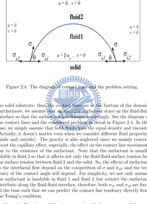
2.4 The diagram of contact lines and the problem setting. . . 26

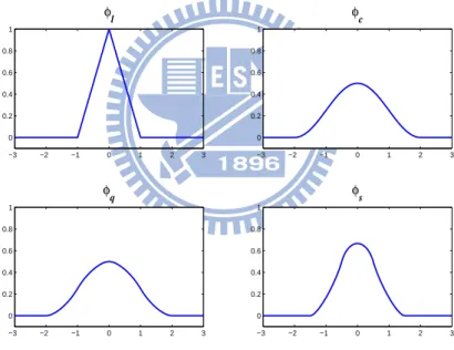
3.1 (a) Hat function. (b) Cosine approximation. (c) Second-order approximation with 4-point support. (d) Second-order ap-proximation with 3-point support. . . 43 4.1 A diagram of the staggered grid. . . 45

5.1 Comparison of stretching factor |Xα| with (UA = 0, dashed

line) and (UA_{6= 0, solid line), where h = 1/128. . . 64}

5.2 The time evolution of a bubble in a quiescent flow. The dash-line is the configuration of the steady state which is a circle

with re = 0.4243. (a) Relative error of area loss. (b) Total

length of the bubble. . . 65 5.3 (a) A bubble with bulk surfactant in the second quadrant

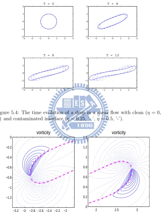
moves to the left-top corner of the box. (b) The correspond-ing evolution of surfactant concentration of (a). (c) A bubble with bulk surfactant in the third quadrant moves to the left-bottom corner of the box. (d) The corresponding evolution of surfactant concentration of (c). . . 66 5.4 The time evolution of a drop in a shear flow with clean (η = 0,

’.’) and contaminated interface (η = 0.25, ’-.’, η = 0.5, ’-’). . . 68 5.5 The vorticity plot for the drop with surfactant near the left

and right tips (η = 0.5, T = 12). . . . 68

5.6 Distributions of the surfactant concentration (left) and the corresponding surface tension (right). Notations and

parame-ters are same as in Fig. 5.14. . . 70

5.7 The corresponding capillary force (left) and Marangoni force

(right). Notations and parameters are same as in Fig. 5.14. . 71

5.8 (a) Total mass of the surfactant. (b) Time plot of m(t)−m(0). (c) Total area of the bubble. (d) Total length of the interface. Notations and parameters are same as in Fig. 5.14. . . 72 5.9 The time evolution of a bubble under a shear flow with linear

(’.’) and nonlinear (’-’) equation of state. . . 73

5.10 Distributions of the surfactant concentration (left) and the corresponding surface tension (right). Notations and parame-ters are same as in Fig. 5.9. . . 73 5.11 The corresponding capillary force (left) and Marangoni force

(right). Notations and parameters are same as in Fig. 5.9. . . 74 5.12 (a) Total mass of the surfactant. (b) Time plot of m(t)−m(0).

(c) Total area of the bubble. (d) Total length of the interface.

Notations and parameters are same as in Fig. 5.9. . . 74

5.13 The effect of capillary number Ca on the deformation of the bubble. (Ca = 0.05 : ’.’, Ca = 0.25: ’-’, Ca = 0.5: ’-.’,

Ca = 1.0: ’–’) . . . 75

5.14 The time evolution of a hydrophilic drop with clean (η = 0,

dashed line) and contaminated interface (η = 0.3, solid line). 76

5.15 The velocity field for the drop with surfactant near the left and right contact lines (η = 0.3, T = 1.5625). . . 77

5.16 Distribution of the surfactant concentration (top) and the cor-responding surface tension (bottom). . . 78 5.17 (a) Left contact line speed of the drop. (b) Right contact line

speed of the drop. (c) Contact angle of the drop. (d) Total length of the drop. Notations and parameters are same as in Fig. 5.14. . . 79 5.18 The time evolution of a hydrophobic drop with clean (η = 0,

dashed line) and contaminated interface (η = 0.3, solid line). 80

5.19 The velocity field for the drop with surfactant near the left

and right contact lines (η = 0.3, T = 1.5625). . . . 81

5.20 (a) Left contact line speed of the drop. (b) Right contact line speed of the drop. (c) Contact angles of the drop. (d) Total length of the drop. Notations and parameters are same as in Fig. 5.18. . . 82 5.21 Wettability and the initial drop set up. . . 83 5.22 The time evolution of a hydrophilic drop with clean (η = 0,

dashed line) and contaminated interface (η = 0.3, solid line). 83

5.23 The velocity field for the drop with surfactant near the left

and right contact lines at T = 1.0938, 3.5938. . . . 84

5.24 Distribution of the surfactant concentration (top) and the cor-responding surface tension (bottom). . . 85 5.25 (a) Left contact line speed of the drop. (b) Right contact line

speed of the drop. (c) Left contact angle of the drop. (d)

Right contact angle of the drop. . . 86

5.26 (a) A rising bubble with Eo = 0.1. (b) A rising bubble with

Chapter 1

Introduction

The real world is abundant in phenomena of free surfaces, interfaces and mov-ing boundaries (generally called interfaces), that interact with a surroundmov-ing substances, like gas, fluid, or solid. These interfaces separate one fluid from another, for instance air and water form the case of bubbles or free surface flows, and behave as boundaries between two materials of different physical properties. In some respects, the interface may be a rigid wall that moves with some specified time dependent motion, or an elastic membrane that deforms and stretches in response to the fluid motion. In addition, motion of interface may involve not only the dynamics of the liquid and surrounding air but also their interaction with adjacent solid surfaces. Many industrial processes, ranging from spin coating of microchips to de-icing of aircraft sur-faces, rely on the ability to control these interactions.

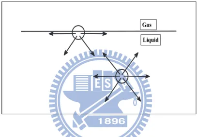
Fluid flows with moving interfaces play important roles in many scientific, biomedical, and engineering applications. The interaction of muscle tissue with blood in the heart and arteries, coating of solid substrates with liquids, film boiling and crystal growth, micro-organisms utilize for locomotion the anisotropic drag properties of their long flexible flagella, are part of interest-ing applications. If an incompressible fluid flow contains an interface and the interface is between fluid 1 and fluid 2, then the flow often refers to be a free surface flow. The position of the interface is determined by the capillary force (a force acts in the direction perpendicular to the tangent plane of an inter-face point), which results from the balance between the normal stress and the surface tension on the interface. Generally speaking, these problems are usu-ally described by the time-dependent incompressible Navier-Stokes equations together with interface jump conditions (can be viewed as a balance of forces on the interface). These types of problems are generally called free-boundary problems, multi-phase flow problems or interfacial flow problems.

1.1

Surface tension

In the microscopic sense of a matter, molecules attract one another all the time. When the attraction is stronger than thermal agitation, molecules switch from a gas phase to a more dense phase, so called a liquid. A molecule in the midst of a liquid interacts with all its neighbors and finds itself in a ”happy” state. By contrast, a molecule that floats at the surface loses half of its cohesive interactions, see Fig 1.1, and becomes ”unhappy”. That is

L iq u id G a s

Figure 1.1: An unhappy molecule at the surface: it is missing half its attrac-tive interaction.

the fundamental reason that liquids adjust their shape in order to expose the smallest possible surface area.

In physics, a liquid molecule is in an unfavorable energy state when it moves to the surface. If the cohesion energy per molecule is U inside the liquid, a molecule sitting at the surface goes short of energy roughly U/2. The surface tension is a direct measure of this energy shortfall per unit surface

area. If r is the molecule’s size and r2 _{is its exposed area (like one face of a}

cube), the surface tension is of order σ ∼= U/(2r2_{). For most oils, for which}

the interactions are of the van der Waals type, we have U ∼= kT , which

is the thermal energy. At a temperature of 25◦_{C, kT is equal to 1/40 eV ,}

which gives σ = 20 mJ/m2_{. Because water involves hydrogen bonds, its}

surface tension is larger (σ ≈ 72 mJ/m2_{). For mercury, which is a strongly}

equivalently be expressed in units of mN/m. Similarly, the surface energy between two non-miscible liquids a and b is characterized by an interfacial

tension σab. Table 1.1 [47] lists the surface tensions of some ordinary liquids

(including those usually used in the experiments of related applications), as

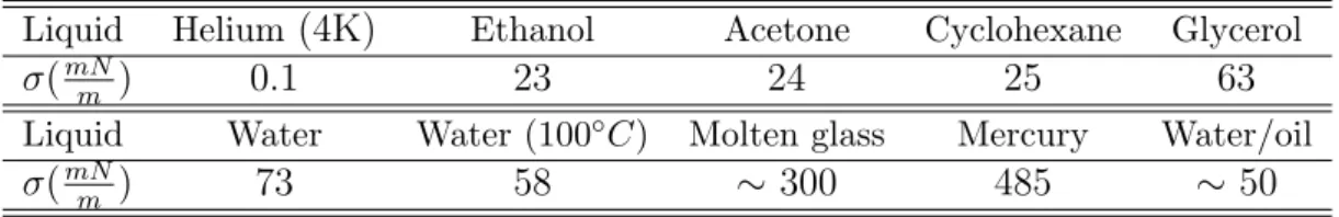
Table 1.1: Surface tension of a few common liquids (at 20◦_{C unless otherwise}

noted) and interfacial tension of the water/oil system.

Liquid Helium (4K) Ethanol Acetone Cyclohexane Glycerol

σ(mN

m ) 0.1 23 24 25 63

Liquid Water Water (100◦_{C) Molten glass Mercury Water/oil}

σ(mN

m ) 73 58 ∼ 300 485 ∼ 50

well as the interface tension between water and oil. Although its origin can be explained at the molecular level, the surface tension σ is a macroscopic

( a ) ( b )

Figure 1.2: (a) Two bugs stay on the water-air surface. (b) A cross-sectional view of one leg of a bug.

parameter defined on a macroscopic scale. In Fig. 1.2(a), two waterstriders can mat on the water mainly due to the effect of surface tension. One can think the surface tension as the force acting parallel to the water-air surface

and perpendicular to the line (the long leg of the bug), see Fig. 1.2(b), fs

and fw reach a balance so that the leg is static on the water-air interface.

Suppose one wants to distort a liquid to increase its surface area by an amount

dA. The work required is proportional to the number of molecules that must

be brought up to the surface, i.e., to dA; and one can write:

δW = σ dA

where σ is the surface (or interfacial) tension. Dimensionally, [σ] = E/L2_.

The surface tension σ is thus expressed in units of mJ/m2_{. In words, σ is}

the energy that must be supplied to increase the surface area by one unit.

1.2

Surfactant

Surfactants are the most versatile products of the chemical industry, ap-pearing in various products such as the motor oils in the automobiles, the pharmaceutics for patients, the detergents for cleaning our laundry and our homes, and the flotation agents used in benefit of ores [9]. In a liquid-liquid system, surfactant allows small droplets to be formed and used as an emul-sion. Surfactant also plays an important role in water purification and other applications where micro-sized bubbles are generated by lowering the surface tension of the liquid-gas interface. In microsystems with the presence of in-terfaces, it is extremely important to consider the effect of surfactant since in such cases the capillary effect dominates the inertia of the fluids [51]. The last decades have seen the extension of surfactant applications to such high-technology areas as electronic printing, magnetic recording, biohigh-technology, micro-electronics, and viral research.

An example of surfactant for babies is the surfactant production in the unborn baby’s lung. In pregnancy, the components of surfactant start to appear at approximately week twentieth, however it is not until much later in pregnancy that the surfactant becomes mature enough to work correctly. In the lungs, surfactant is a complex substance containing phospholipid and four different types of surfactant proteins: hydrophilic (water-attracting) pro-teins SP-A and SP-D and the hydrophobic (water-repelling) propro-teins SP-B and SP-C. These latter proteins, SP-B and SP-C (also present in Curosurf), are essential for the uniform spreading of the surfactant throughout the lung. The main role of surfactant is to prevent collapse of the alveoli thereby re-ducing the effort needed to expand the lungs during inspiration (breathing in) and allow gas exchange to take place. Surfactant therefore helps breath-ing to be relatively effortless. Durbreath-ing expiration (breathbreath-ing out) the lungs have a tendency to collapse, if they are allowed to do so then a much greater inspiratory effort is required to open them with the next breath. Surfactant

Figure 1.3: The diagram of the alveoli.

prevents this by reducing surface tension throughout the lung; surface ten-sion is the force present within the alveoli of the lungs that courses them to collapse and stick together during expiration. Surfactant forms a very thin film which covers the surface of the alveolar cells; the components of surfactant work together to reduce surface tension and therefore reduce the tendency of the alveoli to collapse during expiration. The lungs are less stiff (improved pulmonary compliance) and therefore reduced effort is needed to expand the lungs and making breathing easier. The natural production of surfactant increases at approximately week 30 to 32 and babies born after the end of the 32nd week usually have sufficient surfactant to breath normally.

1.3

Reduction of surface tension by

surfac-tants

Surfactant are surface active agents that adhere to the fluid interface and affect the interfacial tension. Reduction of surface or interfacial tension is one of the most commonly measured properties of surfactants in solution. Since it depends directly on the replacement of molecules of solvent at the interface by molecules of surfactant, and therefore on the surface (or interfacial) excess concentration of the surfactant, as shown by the Gibbs equation

dσ = −X

i

it is also one of the most fundamental of interfacial phenomena.

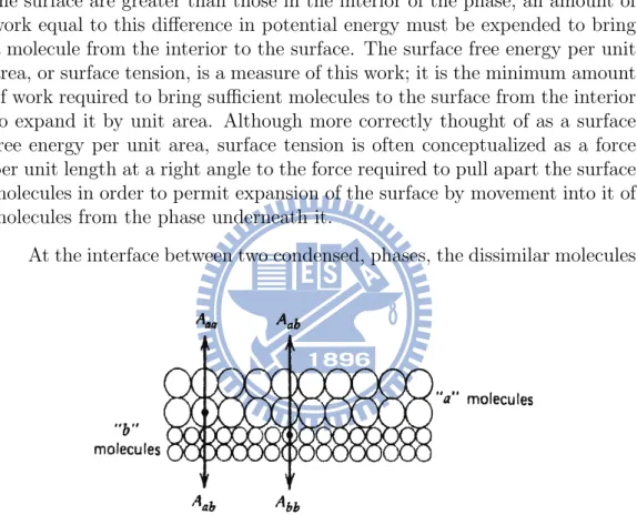
As we know, the molecules at the surface of a liquid have potential ener-gies greater than those of similar molecules in the interior of the liquid. (This is because attractive interactions of molecules at the surface with those in the interior of the liquid are greater than those with the widely separated molecules in the gas phase.) Because the potential energies of molecules at the surface are greater than those in the interior of the phase, an amount of work equal to this difference in potential energy must be expended to bring a molecule from the interior to the surface. The surface free energy per unit area, or surface tension, is a measure of this work; it is the minimum amount of work required to bring sufficient molecules to the surface from the interior to expand it by unit area. Although more correctly thought of as a surface free energy per unit area, surface tension is often conceptualized as a force per unit length at a right angle to the force required to pull apart the surface molecules in order to permit expansion of the surface by movement into it of molecules from the phase underneath it.

At the interface between two condensed, phases, the dissimilar molecules

Figure 1.4: Simplified diagram of the interface between two condensed phases

a and b.

in the adjacent layers facing each other across the interface (Fig. 1.4) also have potential energies different from those in their respective phases. Each molecule at the interface has a potential energy greater than that of a similar molecule in the interior of its bulk phase by an amount equal to its interaction energy with the molecules in the interior of its bulk phase minus its interac-tion energy with the molecules in the bulk phase across the interface. For most purposes, however, only interactions with adjacent molecules need be

taken into account. If we consider an interface between two pure liquid phases

a and b (Fig. 1.4), then the increased potential energy of the a molecules at

the interface over those in the interior of that phase is Aaa and Aab, where

Aaa symbolizes the molecular interaction energy between a molecules at the

interface and similar molecules in the interior of the bulk phase and Aab

sym-bolizes the molecular interaction energy between a molecules at the interface and b molecules across the interface. Similarly, the increased potential of b

molecules at the interface over those in the interior is Abb−Aab. The increased

potential energy of all the molecules at the interface over those in the interior

of the bulk phases, the interfacial free energy, is then (Aaa−Aab)+(Abb−Aab)

or Aaa + Abb− 2Aab, and this is the minimum work required to create the

interface. The interfacial free energy per unit area of interface, the interfacial

tension σI is then given by the expression

σI = σa+ σb − 2σab, (1.1)

where σa and σb are the surface free energies per unit area (the surface

ten-sions) of the pure liquids a and b, respectively, and σabis the a − b interaction

energy per unit area across the interface.

The value of the interaction energy per unit area across the interface σab

is large when molecules a and b are similar in nature to each other (e.g., water

and short-chain alcohols). When σab is large, we can see from equation (1.1)

that the interfacial tension σI will be small; when σab is small, σI is large.

The value of the interfacial tension is therefore a measure of the dissimilarity of the two types of molecules facing each other across the interface.

In the case where one of the phases is a gas (the interface is a surface), the molecules in that phase are so far apart relative to those in the condensed phase that tensions produced by molecular interaction in that phase can be

disregarded. Thus if phase a is a gas, σa and σab can be disregarded and

σI ≈ σb, the surface tension of the condensed phase b.

When the two phases are immiscible liquids, σa and σb, their respective

surface tensions, are experimentally determinable, pennitting the evaluation

of σab, at least in some cases. If one of the phases is solid, on the other hand,

experimental evaluation of σab is difficult, if not impossible. However here,

too, the greater the similarity between a and b in structure or in the nature of their inkrmolecular forces, the greater the interaction between them (i.e.,

the greater the value of σab) and the smaller the resulting interfacial tension

between the two phases. When 2σab becomes equal to σa+ σb, the interfacial

region disappears and the two phases spontaneously merge to form a single one.

If we now add to a system of two immiscible phases (e.g., heptane and

Figure 1.5: Diagrammatic representation of heptane-water interface with adsorbed surfactant.

water), a surface-active agent that is adsorbed at the interface between them, it will orient itself there, mainly with the hydrophilic group toward the wa-ter and the hydrophobic group toward the heptane (Fig. 1.5). When the surfactant molecules replace water and/or heptane molecules of the original interface, the interaction across the interface is now between the hydrophilic group of the surfactant and water molecules on one side of the interface and between the hydrophobic group of the surfactant and heptane on the other side of the interface. Since these interactions are now much stronger than the original interaction between the highly dissimilar heptane and water molecules, the tension across the interface is significantly reduced by the pres-ence there of the surfactant. Since air consists of molecules that are mainly non-polar, surface tension reduction by surfactants at the air-aqueous solu-tion interface is similar in many respects to interfacial tension reducsolu-tion at the heptaneVaqueous solution interface.

We can see from this simple model why a necessary but not sufficient condition for surface or interfacial tension reduction is the presence in the surfactant molecule of both lyophobic and lyophilic portions. The lyophobic portion has two functions: (1) to produce spontaneous adsorption of the sur-factant molecule at the interface and (2) to increase interaction across the interface between the adsorbed surfactant molecules there and the molecules in the adjacent phase. The function of the lyophilic group is to provide strong interaction between the molecules of surfactant at the interface and the molecules of solvent. If any of these functions is not performed, then the marked reduction of interfacial tension characteristic of surfactants will

probably not occur. Thus, we would not expect ionic surfactants containing hydrocarbon chains to reduce the surface tensions of hydrocarbon solvents, in spite of the distortion of the solvent structure by the ionic groups in the surfactant molecules. Adsorption of such molecules at the airhydrocarbon interface with the ionic groups oriented toward the predominantly non-polar air molecules would result in decreased interaction across the interface, com-pared to that with their hydrophobic groups oriented toward the air.

For significant surface activity, a proper balance between lyophilic and lyophobic character in the surfactant is essential. Since the lyophilic (or lyophobic) character of a particular structural group in the molecule varies with the chemical nature of the solvent and such conditions of the system as temperature and the concentrations of electrolyte and/or organic additives, the lyophilic-lyophobic balance of a particular surfactant varies with the sys-tem and the conditions of use. In general, good surface or interfacial tension reduction is shown only by those surfactants that have an appreciable, but limited, solubility in the system under the conditions of use. Thus surfac-tants which may show good surface tension reduction in aqueous systems may show no significant surface tension reduction in slightly polar solvents such as ethanol and polypropylene glycol in which they may have high solubility.

1.4

Surfactant in moving contact line

prob-lems

In our daily lives, there are full of the motion of liquid under the influence of surface tension. For example, drink a cup of coffee, take a shower, wash clothes, design a thermometer, wax cars, or cook with nonstick cook ware, etc.. These phenomena always involve a key, the interface of the two fluid phases intersects the solid phase to introduce the motion of a contact line, where a triple juncture of the solid/gas, solid/liquid, and liquid/gas inter-faces. A typical paradox arises from no-slip boundary conditions near the contact line, implies that an infinite force is required to move a contact line [8, 47]. In recent decades, many scientists put lots of effort on curing this paradox. Several models have been proposed to study the motion of moving contact lines. Most of them involve adding an additional effect on a micro-scopic length-scale, for instance, weakening the no-slip boundary condition via a slip condition effective at small scales [11, 12, 43] or incorporating the effect of long-range Van der Waals forces between the liquid and solid.

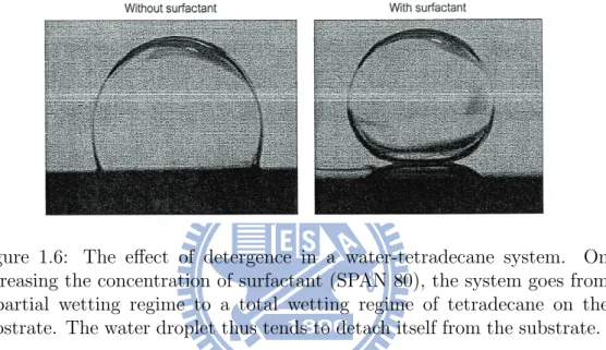
can change the wetting properties by altering the value of the contact angle. This simple fact has found may interesting applications in our daily life and industrial processes. For example, we add detergents (surfactant) in washing machine to clean our clothes more effectively. The detergent helps to remove drops of grease from clothes by increasing the contact angle (measured from inside the drop). An idealization of this problem can be found in a photo shown in Fig. 1.6 [51] or a figure in [14] where it is demonstrated that a

Figure 1.6: The effect of detergence in a water-tetradecane system. On increasing the concentration of surfactant (SPAN 80), the system goes from a partial wetting regime to a total wetting regime of tetradecane on the substrate. The water droplet thus tends to detach itself from the substrate. drop on clothes can become less wetting (from the drop point of view) by in-creasing surfactant concentration. By adding surfactant, a drop which sticks to clothes becomes less sticky and the water currents can wash away the drop readily. The physical situation corresponding to this idealized system includes a solid-drop (grease)-water system and the surfactant. Mathemati-cally, as discussed more detail in the main text of this dissertation, this is a moving contact line problem since the solid-drop (grease)-water triple inter-section forms a contact line. One of the main issues we will try to address in this dissertation is how surfactant, by changing the contact angle, affects the movement of the contact line.

1.5

Immersed boundary method

The immersed boundary (IB) method proposed by Peskin [35], has been applied successfully to blood-valve interaction and other biological problems. The IB formulation employs a mixture of Eulerian and Lagrangian variables,

where the immersed boundary is represented by a set of discrete Lagrangian markers embedding in the Eulerian fluid domain. Those markers can be treated as force generators to the fluid while being carried by the fluid motion. The interaction between the Lagrangian force generators (markers) and the fluid motion, described by variables defined on the fixed Eulerian grid, is linked by a properly chosen discretized delta function. Most IB applications in the literature belong to the fluid-structure problems, and they can be found in a recent review of Peskin [36]. However, there is comparatively less work on the application of the IB method to viscous, incompressible multi-phase flow problems. Perhaps the most successful one is the front-tracking method proposed by Tryggvason et al. [53, 52] which uses an approach similar to the immersed boundary method.

1.6

Numerical experiments

In the case of interfacial flows with surfactant, Ceniceros [5] used a hybrid level set and front tracking approach to study the effects of surfactant on the formation of capillary waves. Lee and Pozrikids [30] used Peskin’s im-mersed boundary idea to study the effects of surfactant on the deformation of drops and bubbles in Navier-Stokes flows. The surfactant convection-diffusion equation in these papers is based on the formulation proposed by Wong et al. [54], and the conservation of total mass of surfactant on the interface has not been rigorously investigated numerically.

James and Lowengrub [24] have proposed a surfactant-conserving volume-of-fluid method for interfacial flows with insoluble surfactant. Instead of solving the surfactant concentration equation based on Stone’s derivation [49] directly, the authors relate the surfactant concentration to the ratio of the surfactant mass and surface area so that they are tracked independently. The method has been applied to study the axis-symmetric drop deformation in extensional flows. Recently, Xu et al. [56] develop a level-set method for interfacial Stokes flows with surfactant. Their method couples surfactant transport, solved in an Eulerian domain [57] with Stokes flow field, solved by the immersed interface method [28] with jump conditions across the in-terface. However, the method does not conserve the mass automatically and numerical scaling is used to enforce the conservation of surfactant on the interface numerically. Recently, Muradoglu and Tryggvason [33] have proposed a front-tracking method for computation of interfacial flows with soluble surfactant. They consider the axis-symmetric motion and deforma-tion of a viscous drop moving in a circular tube.

Numerical simulation of two-phase flows with moving contact lines have also been developed in the literature. Finite element method [39], level set method [48], front tracking method [20], volume-of-fluid method [45, 50, 58], phase field method [23, 42], sharp interface Cartesian grid method [26] and molecular dynamics [40, 41, 43] have been tools to address these problems. However, to the best of our knowledge there is no numerical result taking the contaminant into account in the fluid, even only on the interface. In hydrodynamic cleaning, a shear flow is exploited for the removal of remnant droplets of a contaminant or impurity. The removal of droplets from the narrow passages of a porous medium determines the efficiency of tertiary oil recovery and plays an important role in the micro-mechanics of groundwater flow.

Chapter 2

Mathematical model for

interfacial flow

The essential purpose of this chapter is to derive the mathematical model for physical problems we are interested in. First, we derive the governing equations of fluid flows which result from invoking the physical laws of con-servation of mass, and momentum. Basically, we use the continuum method, which ignores individual molecules and assumes that the fluid consists of continuous matter, to describe equations which govern the motion of fluid. Since there is an interface immersed in the fluid, we use two reference frames simultaneously, the Eulerian framework is employed for fluid variables while variables defined on the interface are based on the Lagrangian framework. A general theorem, called the Reynolds’ transport theorem [7], is used to re-late derivatives of Lagrangian and Eulerian frameworks to yield the so-called continuity equation and the Navier-Stokes equations. Further, the boundary conditions across a interface for a two-phase flow will be determined, and it can be converted into a singular force by the use of a continuum surface forces formulation [4, 35].

Next, the conservation of mass of surfactant concentration comes from its insolubility on the interface, and the corresponding governing equation will be represented in a simple form [31]. For moving contact line problems, the interface movement involves not only the fluid-fluid surface tension but surface tensions between solid substrate and liquids. A driver called the un-balanced Young force for the contact line will be introduced to mimic the tendency of the Young condition. To close the system, appropriate boundary conditions, respectively, for fluid field [15] (especially Navier-slip boundary condition for the moving contact line problems) and surfactant concentration, will be introduced at the end of this chapter.

2.1

Governing equations of bulk fluids

We first introduce the concept of a control volume V which is arbitrary in shape, and each conservation principle is applied to the integral over a control volume. The result of applying each conservation principle will be an

integro-differential equation of the type R_V LψdV = 0 where L is some differential

operator and ψ is some property of fluid, like density or velocity. Since V is arbitrarily chosen, the only way this equality can be satisfied is to set Lψ = 0, which is a differential equation of the corresponding conservation law. The following is a principal theorem, so-called Reynolds’ transport theorem, to derive differential equations of conservation laws.

Theorem. Suppose that ψ is any property of the fluid dependent on space

and time, i.e. ψ = ψ(x, t), and V is the control volume, then the rate of change of the integral of ψ is

D Dt Z V (t) ψ(x, t)dV = Z V (t) µ ∂ψ ∂t + ∇ · (ψu) ¶ dV, (2.1)

where D/Dt is the lagrangian derivative and u is the velocity of the control volume.

proof: Assume that the control volume is a function of t, and V (t) is the control volume at time t, then V (t + δt) is the control volume after flowing a small time δt away from t. By definition of the differentiation,

D Dt Z V (t) ψ(x, t)dV = lim δt→0 1 δt µZ V (t+δt) ψ(x, t + δt)dV − Z V (t) ψ(x, t)dV ¶ = lim δt→0 1 δt µZ V (t+δt) ψ(x, t + δt) − ψ(x, t)dV + Z V (t+δt)−V (t) ψ(x, t)dV ¶ ,

the first term of the right-hand side is actually the integral of the partial derivative of ψ(x, t) with respect to t, and the second term can be converted to a surface integral by the use of the approximation dV = u · nδtdS, there-fore, lim δt→0 1 δt Z V (t+δt)−V (t) ψ(x, t)dV = lim δt→0 1 δt Z S(t) ψ(x, t)u · nδtdS.

Moreover, the divergence theorem transfer the surface integral back to a volume integral Z S(t) ψ(x, t)u · ndS = Z V (t) ∇ · (ψ(x, t)u) dV

2.1.1

Conservation of mass

The conservation of mass is a fundamental concept of physics. Its main spirit states that mass can neither be created nor destroyed except the spe-cial theory of relativity of Albert Einstein, the mass of a body changes as the energy possessed by the body changes. Such nuclear reactions usually occur in subatomic phenomena, and matter may be created, for instance, by the materialization of a photon (quantum of electromagnetic energy) into an electron-positron pair; or it may be destroyed, by the annihilation of this pair of elementary particles to produce a pair of photons.

To comprehend the conservation of mass in fluid mechanics, we consider a specific mass of fluid whose volume V is arbitrarily chosen. This piece of fluid is followed as it flows, meantime, its shape or size will be changed. Suppose there are no nuclear reactions in the process, the principle of mass conservation means that no matter this given piece of fluid changes its size or shape, its mass will remain the same. The mathematical equivalence of the statement of mass conservation is to take the lagrangian derivative D/Dt to

the mass of fluid contained in V , which is R_V ρdV , equal to zero, where ρ is

the density per unit volume. That is, the equation which expresses conser-vation of mass is D Dt Z V ρdV = 0. (2.2)

By use of Eq. (2.1), we transfer a derivative in lagrangian manner of an integral to an integral of derivatives in eulerian manner

D Dt Z V ρdV = Z V µ ∂ρ ∂t + ∇ · (ρu) ¶ dV = 0,

and since V is arbitrary, we obtain a local differential form of conservation of mass as

∂ρ

∂t + ∇ · (ρu) = 0. (2.3)

Alternatively, using the Einstein notation convention, (2.3) can be rewritten as ∂ρ ∂t + ∂ ∂xk (ρuk) = 0. (2.4)

Note that this partial differential equation forces the velocity field to be at least continuous. So, Eq. (2.3) is usually called the continuity equation.

2.1.2

Conservation of momentum

The conservation of momentum is another important concept of physics along with the conservation of mass. Momentum is defined to be the product of the mass of an object and its corresponding velocity. The conservation of momentum states that within some problem domain, the amount of momen-tum remains constant. In other words, momenmomen-tum is neither created nor destroyed, but only changed through the action of forces. In fact, the princi-ple of conservation of momentum is an application of Newton’s second law of motion to an object. In fluid mechanics, Newton’s second law of motion can be easily derived by an element of the fluid. That is, if we consider a given mass of fluid in a lagrangian framework, the rate of change of the momentum of the fluid mass is equal to the net external force acting on the mass. Some people prefer to think of forces only and restate this law in the form that the inertia force is equal to the net external force acting on the element.

Basically, the external forces acting on a mass of the fluid can be simply categorized into two classes. One is the class of body forces, such as gravita-tional or electromagnetic forces. The other is the class of surface forces, such as pressure forces or viscous stresses. Let f be a vector which represents the resultant of the body forces per unit mass, then the net external body force

acting on a mass of volume V is R_V ρf dV . On the other hand, if a surface

vector T represents the resultant surface force per unit area, then the net

external surface force acting on the surface S containing V is R_STdS. Also,

we assume that the mass per unit volume is ρ and its momentum is ρu,

so that the momentum contained in the volume V is R_V ρudV . According

to statements of Newton’s second law of motion, the rate of the change of momentum (or inertia force) is equal to the sum of the resultant forces. If the mass of the arbitrarily chosen volume V is observed in the lagrangian framework, the rate of change of momentum of the mass contained within V

will be (D/Dt)R_V ρudV . Therefore, we can obtain a mathematical equation

which arises from imposing the physical law of conservation of momentum in the form D Dt Z V ρudV = Z S TdS + Z V ρf dV, (2.5)

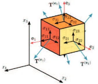
In general, we can use a stress tensor [7] to represent surface forces acting on the fluid, and there are nine components of stress at any given point, one normal component and two shear components on each coordinate plane. These nine components of stress can be easily illustrated by the use of a cubical element in Fig. 2.1, then the stress components will act at a point as the length of the cube tends to zero. In Fig. 2.1 the cartesian coordinates

Figure 2.1: The diagram of nine components of stress.

(x, y, z) have been denoted by (x1, x2, x3). This allows us to describe

the components of stress as a double-subscript notation. In this notation, a

particular component of the stress may be represented by the quantity σij,

in which the first subscript indicates that this stress component acts on the

plane xi = C, where C is a constant, and the second subscript indicates that

it acts in the xj-direction. The fact that the stress maybe represented by the

quantity σij, in which i and j may be 1, 2, or 3, means that the stress at a

point may be represented by a tensor of rank 2. However, it was observed that there would be a vector force at each point on the surface of the control volume, and this force was represented by T. The surface force vector T may

be related to the stress tensor σij as follows: The three stress components

acting on the plane x1 = constant are σ11, σ12, and σ13. Since the unit

normal vector acting on this surface is n1, the resulting force acting in the

x1 direction is T1 = σ11n1. Likewise, the forces acting in the x2 direction and

the x3 direction are, respectively, T2 = σ12n1 and T3 = σ13n1. Then, for an

arbitrarily oriented surface whose unit normal has components n1, n2, and

n3, the surface force will be given by Tj = σijni in which i is summed from

1 to 3. That is, in tensor notation the equation expressing conservation of momentum becomes D Dt Z V ρujdV = Z S σijnidS + Z V ρfjdV

Again, the left-hand side of this equation can be converted to a volume integral of only eulerian derivatives by using Eq. (2.1), meanwhile, the surface integral on the right-hand side can be changed to a volume integral by making use of Gauss’ theorem. In this way the equation which evolved from Newton’s second law becomes

Z V µ ∂ ∂t(ρuj) + ∂ ∂xk (ρujuk) ¶ dV = Z V ∂σij ∂xi dV + Z V ρfjdV

Collect these volume integrals to express this equation in the formR_V{}dV =

0, where the integrand is a differential equation in eulerian coordinates. As before, the arbitrariness of the control volume V implies that the integrand of the above integro-differential equation have to present the basic law of dynamics in an equivalent differential equations

∂ ∂t(ρuj) + ∂ ∂xk (ρujuk) = ∂σij ∂xi + ρfj,

If we consider ρujuk as the product of ρuk and uj, and expand the left-hand

side of the equation above, we obtain

ρ∂uj ∂t + uj ∂ρ ∂t + uj ∂ ∂xk (ρuk) + ρuk ∂uj ∂xk = ∂σij ∂xi + ρfj

Note that the sum of the second and third terms on the left-hand side of this equation is zero due to the continuity equation (2.4). With this simplification, the expression of conservation of momentum becomes

ρ∂uj ∂t + ρuk ∂uj ∂xk = ∂σij ∂xi + ρfj (2.6)

It is useful to recall that this equation came from an application of Newton’s second law to an element of the fluid. The left-hand side of Eq. (2.6) rep-resents the rate of change of momentum of a unit volume of the fluid (or the inertia force per unit volume). The first term is the familiar temporal acceleration term, while the second term is a convective acceleration and ac-counts for local accelerations even when the flow is steady. Note also that this second term is nonlinear, since the velocity appears quadratically. On the right-hand side of Eq. (2.6) are the forces which are causing the acceler-ation. The first of these is due to the gradient of surface shear stresses and the second is due to body forces, such as gravity, which act on the mass of the fluid. A clear understanding of the physical significance of each of the terms in Eq. (2.6) is essential when approximations to the full governing equations must be made. In the following, we will list some assumptions and

the surface-stress tensor σij will be related to an expression of pressure and

1. When the fluid is at rest, the stress is hydrostatic and the pressure exerted by the fluid is the thermodynamic pressure. This implies that

the stress tensor σij is of the form

σij = −pδij + τij (2.7)

where τij depends on the motion of the fluid only and is called the

shear-stress tensor. The quantity p is the thermodynamic pressure and

δij is the Kronecker delta.

2. The stress tensor σij is linearly related to the deformation-rate tensor

ekl and depends only on that tensor. This is the distinguishing feature

of newtonian fluids. There are nine elements in the shear-stress tensor

τij, and each of these elements may be expressed as a linear combination

of the nine elements in the deformation-rate tensor ekl (just as a vector

may be represented as a linear combination of components of the base

vectors). That is, each of the nine elements of τij will in general be a

linear combination of the nine elements of ekl so that 81 parameters

are needed to relate τij to ekl. This means that a tensor of rank 4 is

required so that the general form of τij will be

τij = αijkl

∂uk

∂xl

(2.8) 3. Since there is no shearing action in a solid body rotation of the fluid,

no shear stresses will act during such a motion. Then

τij = 1 2βijkl µ ∂uk ∂xl − ∂ul ∂xk ¶ (2.9) 4. There are no preferred directions in the fluid, so that the fluid properties are point functions. This condition is the so-called condition of isotropy, which guarantees that the results obtained should be independent of the orientation of the coordinate system chosen. The most general isotropic tensor of rank 4 is of the form, see appendix in [7],

λδijδkl+ µ (δikδjl+ δilδjk) + γ (δikδjl− δilδjk) (2.10)

Using the fact that δkl = 0 unless l = k, the expression fro the

shear-stress tensor becomes

τij = λδij ∂uk ∂xk + µ µ ∂ui ∂xj +∂uj ∂xi ¶ (2.11) Thus the constitutive relation for stress in a newtonian fluid becomes

σij = −pδij + λδij ∂uk ∂xk + µ µ ∂ui ∂xj + ∂uj ∂xi ¶ (2.12)

2.2

A two-dimensional incompressible two-phase

flow

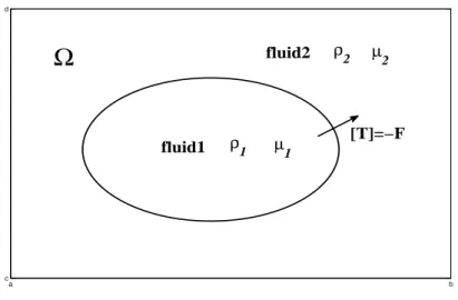
Consider an incompressible two-phase flow problem consisting of fluids 1 and

2 in a fixed two-dimensional square domain Ω = [a, b]×[c, d] = Ω1∪Ω2 where

an interface Σ separates Ω1 from Ω2, see Fig. 2.2. Actually, almost all

ma-terials in reality are compressible to some extent, and the incompressibility refers to flow, not the material property. This means that under certain cir-cumstances, a compressible material can nearly behave as an incompressible flow. Strictly speaking, an incompressible fluid is a fluid which is not reduced in volume by an increase in pressure. With this ideal assumption, the density of the fluid element is a constant as it moves from one point to another. This implies that the material derivative of density is zero, Dρ/Dt = 0. Then Eq. (2.3) can be reduced in the following:

0 = ∂ρ

∂t + ∇ · (ρu) =

Dρ

Dt + ρ∇ · u ⇒ ∇ · u = 0.

Take advantage of the divergence free property of the velocity, λδij∂u_∂xk_k is zero,

then Eq. (2.12) is simply reduced as

σij = −pδij + µ µ ∂ui ∂xj +∂uj ∂xi ¶ .

Since these equation are satisfied in each bulk fluid, we can write the corre-sponding Navier-Stokes equations of the two-phase flow as

ρi µ ∂ui ∂t + (ui· ∇)ui ¶ = ∇ · Ti+ ρifi in Ωi (2.13) ∇ · ui = 0, in Ωi, (2.14)

where for i = 1, 2 in each fluid domain, Ti = −piI + µi(∇ui+ ∇uTi) is the

stress tensor, pi is the pressure, ui is the fluid velocity, ρi is the density, µi

is the viscosity, and f_i is the external force such as the gravitational force.

Jump conditions cross the interface

When two fluids contact with each other, they form a thin layer (a few nanometers for most fluids) due to the influence from the bulk phases. Al-though this layer is very thin, the intermolecular forces acting on it from the bulk phases are so strong that asymmetry in these forces is very important

a b c d

Ω

fluid1 fluid2 µ₂ µ 1 ρ₁ ρ₂ [T]=−F

Figure 2.2: The diagram of a bubble in a two-phase interfacial flow.

for the overall dynamics of the system. For simplicity, the interface is consid-ered as a geometric surface without thickness, and the boundary conditions for the bulk parameters to be formulated on this surface have to incorporate both the universal conservation laws as well as the specific physics of the processes in the interfacial layer for a particular system. Let φ(r, t) be a level function such that φ(r, t) = 0 represents the interface to separate fluid 1 (φ ≤ 0) and fluid 2 (φ ≥ 0) with the superscript + and −, respectively;

n = ∇φ/|∇φ| is a unit normal pointing from fluid 1 to fluid 2.

Suppose that δr is a distance which an element of the interface at position

r traveled in the normal direction n in a very short period δt. Then both φ(r, t) and φ(r + δtn, t + δt) are zeros, and we have

0 = φ(r + δtn, t + δt) = φ(r, t) + ∂φ

∂t (r, t) δt + δrn · ∇φ(r, t) + o(δr, δt),

Divide the above equality by δt and take δt → 0, we obtain an approximation of the shape of the interface

∂φ

∂t + v

s_{· ∇φ = 0, (2.15)}

where vs _{is the normal projection of the interface velocity.}

The conservation laws can be translated into the corresponding boundary conditions in several equivalent ways. Here, an approach based on considering

fluxes across the interface will be used.

Since the interface is very thin and massless (or the density there is of the same order as in the bulk), a sink or source of mass can be neglected compared to the mass fluxes across the boundary. As a result, in the general case of a permeable interface we have the continuity of mass flux across it

ρ+¡_u+_{− v}s¢_{· n = ρ}−¡_u−_{− v}s¢_{· n at φ(r, t) = 0. (2.16)}

Note that Eq. (2.16) holds for both permeable and impermeable interface, it is sufficient to prescribe a specific mass flux for the concerned physics,

ρ+¡_u+_{− v}s¢_{· n = χ, (2.17)}

where χ has to be specified in terms of parameters determining a particular physical mechanism responsible for mass transfer across the interface, such as, chemical reactions, evaporation-condensation, mutual dissolution of fluids, etc. In particular, a case of an impermeable interface has χ = 0, and this implies that

u+_{· n = u}−_{· n,} ∂φ

∂t + u

+_{· ∇φ = 0, at φ(r, t) = 0 (2.18)}

Alternatively, we consider another formulation for the movement of the in-terface and also consider a continuous tangential velocity, then the jump condition of the velocity is

[u]Σ = u|Σ,2− u|Σ,1 = 0. (2.19)

Similarly, the conservation of momentum can be translated into the bound-ary conditions by using the momentum flux tensor Π defined by Π = ρuu−T.

The momentum fluxes in fluid 1 and 2 across a moving interface are n · Π+

and n · Π+_{, respectively, where}

Π± _{= ρ}±¡_u±_{− v}s¢ ¡_u±_{− v}s¢_{− T}±_{. (2.20)}

Note that if the source or sink effect of momentum from the interface is

neglected compared with nΠ±_{, then the momentum flux across an interface}

is continuous:

n · Π+= n · Π−, (2.21)

for instance, flows with very large length scales such as tidal waves, lava flows, large-scale free-surface flows industry, etc. However, in many situations the dynamics of the interfaces contributes significantly to the overall dynamics

of the system, and we have to consider this contribution here.

The source/sink of momentum due to the presence of an interface simply

composes of two components, external forces Fs _{and surface tension σ.}

For the external forces, the interface may possess properties which in a dynamic sense would ”compensate” its negligible thickness. For example, an electrically charged interface with electric current in a electrically neutral and nonconducting fluid can significantly influence the dynamics of the system by an external electromagnetic field. If the interface has no properties con-cerning external forces, then one can neglect the effect from external forces due to the negligible thickness of the interface. For instance, the effect of gravity is proportional to the mass of liquid contained in the interfacial layer and hence practically never pays any role in the interfacial dynamics.

The second way in which an interface can contribute to the overall dy-namics of the system is through its intrinsic dynamic properties the most important being the surface tension. Physically, the surface tension appears as a result of an asymmetric action on the interfacial layer of intermolecular forces from the bulk phases. These forces are singularly strong compared to those considered in fluid mechanics so that their strength compensates the negligible thickness of the interfacial layer making the resultant dynamic effect finite.

Mathematically, σ is a function defined along the interface and, in

Figure 2.3: (a) The surface tension with which an element of the interface acts on its boundary is normal to the boundary and tangential to the interface; it tries to minimize the area of this element. (b) The resultant action of the surface tension on a surface element from a surrounding surface has a normal component if the interface in not flat, and a tangential component if the surface tension varies along the interface.

the framework of fluid-mechanical modeling, it has to be included in a