應用空域與時域腦動態分析於駕駛安全之雙重任務探討

國 立 交 通 大 學

電控工程研究所

博 士 論 文

應用空域與時域腦動態分析於駕駛安全之雙重

任務探討

Spatial and Temporal EEG-based Brain Dynamics

of Dual-Task Driving Performance

研 究 生：陳世安

指導教授：林進燈 博士

應用空域與時域腦動態分析於駕駛安全之雙重任務探討

Spatial and Temporal EEG-based Brain Dynamics of Dual-Task

Driving Performance Performance

研 究 生：陳世安 Student：Shi-An Chen

指導教授：林進燈 博士

Advisor：Dr. Chin-Teng Lin

國立交通大學

電控工程研究所

博士論文

A Dissertation

Submitted to Department of Electrical Engineering

College of Electrical Engineering

National Chiao Tung University

in Partial Fulfillment of the Requirements

for the Degree of Doctor of Philosophy

in

Electrical Control Engineering

January 2011

Hsinchu, Taiwan, Republic of China

應用空域與時域腦動態分析於

駕駛安全之雙重任務探討

學生：陳世安

指導教授：林進燈 博士

國立交通大學電控工程研究所

Chinese Abstract

中文摘要

於行車中的駕駛者之分心發生已經被證實是造成車禍發生的重大原因之 一。因此，本論文建立虛擬實境技術之動態駕車裝置，來模擬真實之駕車環境， 透過分心場景的設計，結合腦電波(Electroencephalogram, EEG)分析來探討駕車行 為下人類分心效應的腦部認知功能與反應變化。在此實驗中，我們建立雙重任務 促使駕駛者造成分心效應，此雙重任務分別為非預期性的車子偏移與數學問題的 出現。為了研究車子偏移與數學任務的交互作用與影響，我們建立了五個不同時 間間隔(Stimulus Onset Asynchrony, SOA)的雙重任務實驗，並分析此雙重任務於 不同五個時間間隔所反應出的行為表現與腦電波動態變化。腦電波訊號分析採用 獨立成份分析演算法(Independent Component Analysis, ICA)來分離出不同獨立成 份為獨立之訊號源，再將特定獨立訊號源套用事件相關頻譜擾動分析(Event Related Spectral Perturbation, ERSP)來觀察時域與頻域響應，藉此了解並比較不同 時間上腦電波的頻譜差異。從我們的研究成果發現，額葉區(Frontal Lobe)之 Theta 頻帶與 Beta 頻帶的能量增強與駕駛者分心效應有正向關係，另外在運動皮質區 (Motor Area)也觀察到 alpha 頻帶與 beta 頻帶能量抑制的發生，此上述成果是由

整合15 位受測者的腦電波資料，也進行統計檢定分析。於行為表現上，我們觀 察到不同時間間隔下反應時間的趨勢，與腦電波能量變化的趨勢是一致的，這說 明了我們所發現的額葉區腦電波的能量增強現象，與行車中駕駛者分心效應發生 有高度相關，而且能量增強越高，分心效應越強。 關鍵字：分心、認知、虛擬實境、不同時間間隔、獨立成份分析演算法、額 葉區、theta 能量增強

Spatial and Temporal EEG-based Brain Dynamics

of Dual-Task Driving Performance

Student: Shi-An Chen

Advisor: Dr. Chin-Teng Lin

Institute of Electrical Control Engineering

National Chiao Tung University

English Abstract

Abstract

Driver distraction is a significant cause of traffic accidents. The aim of this study is to investigate Electroencephalography (EEG) dynamics in relation to distraction during driving. To study human cognition under a specific driving task, simulated real driving using virtual reality (VR) -based simulation and designed dual-task events are built, which include unexpected car deviations and mathematics questions. We designed five cases with different stimulus onset asynchrony (SOA) to investigate the distraction effects between the deviations and equations. The EEG channel signals are first converted into separated brain sources by independent component analysis (ICA). Then, event-related spectral perturbation (ERSP) changes of the EEG power spectrum are used to evaluate brain dynamics in time-frequency domains. Power increases in the theta and beta bands are observed in relation with distraction effects in the frontal cortex. In the motor area, alpha and beta power suppressions are also observed. All of the above results are consistently observed across 15 subjects. Additionally, further analysis demonstrates that response time and multiple cortical EEG power both

changed significantly with different SOA. This study suggests that theta power increases in the frontal area is related to driver distraction and represents the strength of distraction in real-life situations.

Keyword: distraction, cognition, virtual reality (VR), stimulus onset asynchrony

Chinese Acknowledgements

致 謝

本論文的完成，首先要感謝指導教授林進燈博士這六年多來的悉心指 導，讓我學習到許多寶貴的知識，在學業及研究方法上也受益良多。另外 也要感謝口試委員們的的建議與指教，使得本論文更為完整。 其次，感謝國立交通大學腦科學研究中心的柯立偉博士、邱添丁博士、 同學黃騰毅、王俞凱、林弘章的相互砥礪，及所有學長、學弟們在研究過 程中所給我的鼓勵與協助。尤其是柯立偉博士，在理論及程式技巧上給予 我相當多的幫助與建議，讓我獲益良多。 感謝我的父母親對我的教育與栽培及物質上的一切支援，我的岳父岳 母的提攜，感謝我的老婆雅婷在背後默默的支持我並給予我精神上的鼓 勵，妳的支持是我突破瓶頸與樂於接受新事物挑戰的原動力，並使我能安心地 致力於學業，並順利完成論文。此外也感謝兩位姊姊對我不斷的關心與鼓勵。 謹以本論文獻給我的家人及所有關心我的師長與朋友們。

Contents

Chinese Abstract ...ii

English Abstract ...iv

Chinese Acknowledgements ...vi

Contents ...vii List of Tables...ix List of Figures...x 1 Chapter 1 Introduction...1 1.1 Motivation...1 1.2 Relevant Literatures ...2 1.3 Dissertation Organization ...4

2 Chapter 2 Experimental Approach ...5

2.1 Dynamic Driving Environment...5

2.2 EEG Signal Acquisition ...7

2.3 Experimental Design...8 2.3.1 Subject...8 2.3.2 VR Scenario...9 2.3.3 Task Descriptions...10 2.4 Data Analysis ...11 2.4.1 Behavioral Performance...11

2.4.2 Distraction Effects of Dual-task...12

3 Chapter 3 Experimental Results...18

3.1 Behavioral Performance...18

3.2 Independent Component Clustering ...19

3.3 Cluster Analysis ...22 3.3.1 Frontal Cluster ...22 3.3.2 Motor Cluster ...25 3.3.3 Condition Comparison...28 4 Chapter 4 Discussion ...31 4.1 Frontal Cluster ...31 4.2 Motor Cluster ...34

4.3 Other Clusters ...35

4.4 More Behavioral Experiment...36

4.4.1 Subjects...36

4.4.2 Experiment Results ...36

4.5 Dual-task Distraction Effects...40

4.6 Brain Dynamics Related to Behavioral Performance ...43

5 Chapter 5 CNN Implementation ...46

5.1 Cellular Neural Networks (CNN) ...46

5.2 CNN-based Hybrid-order Texture Segregation ...46

5.2.1 Functions of Blocks ...48

5.3 Experimental Results ...52

5.4 Discussion...54

6 Chapter 6 Conclusion ...57

List of Tables

Table 3-1: The normalized response time to deviation and math ...19 Table 3-2: The Number of Components in Different Clusters...22 Table 4-1: Summary data for responding car deviation and answering math equations variable across all trials (2187 trials for each condition), mean response time (Mean, in milliseconds), standard deviation (SD) and accuracy rate (AR). ...37

List of Figures

Fig. 2-1: Pictures showed the dynamic VR driving environment, in the Brain Research Center of National Chiao Tung University, Taiwan, and ROC. A real car in the 3D VR environment was showed in the left picture. The experimental

setup around the steering wheel was showed in the right picture...5

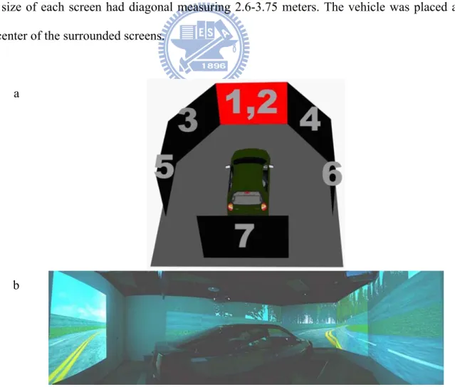
Fig. 2-2: (a) The picture showed the configuration of the 3D surrounded scene. The 3D VR scene consisted of 7 projectors, creating a surrounded view. The frontal screen was overlapped by 2 projector frames in different polarizations, providing a stereoscopic VR scene for 3D visualization. (b) The 3D VR scene. .6 Fig. 2-3: Schematic pictures showed the lateral (A) and top view (B) of international 10-20 system of electrode placement...7

Fig. 2-4: (a) The photomicrograph showed the simulated high way scene. The monotonous scene was designed to reduce the visual disturbance. (b) The illustration of the high way scene. The width of highway from the left to right side was equally divided into 256 units and the width of the car was 32 units. ...9

Fig. 2-5: The illustration shows the relationship of occurrences between the deviation and math tasks. D: deviation task onset. M: math task onset. (a) Case 1: math task presents 400ms before the deviation task onset. (b) Case 2: math and deviation tasks occur at the same time. (c) Case 3: math task presents 400ms after the deviation task onset. (d) Case 4: only math task presents. (e) Case 5: only deviation task occurs. The bottom insets show the onset sequences of the two tasks...11

Fig. 2-6: The flow chart ofEEG data analysis...13

Fig. 2-7: How ICA work for source localization ...14

Fig. 2-8: ICA algorithm can separate 30 sources...14

Fig. 2-9: The illustration of procedures in ERSP analysis. FFT was applied in each window with 256 samples, and there was 244-sample overlap of two adjacent windows. The time-dependent ERSP image was composed of the spectra of each window, and smoothed by 3-window moving average. In the final step, the significant parts of ERSP image were extracted by using bootstrap method. The pink dashed lines: the first event onset. The blue dashed lines: the averaged reaction time to the deviation. The red dashed lines: the averaged response time to math. The black dashed lines: averaged response time for the car returning to the third lane. Color bars showed the magnitude of ERSPs. ...15

Fig. 2-10: The flowchart of component clustering. Components from all subjects were classified into several significant clusters...17

Fig. 3-1: This figure shows the bar charts of normalized response times. (a) for the math task and (b) for deviation task across 15 subjects. The filled black bar: case 1; dark gray bar: case 2; light gray bar: case 3; the open bar: single case. The response time for math task in dual-task cases (case 1, case 2, and case 3) is significantly longer than that for in single task (case 4). The shortest response time for the math onset is in case 4. The response time for deviation task in case 1 is significantly shorter than those in other cases. The longest response time to the deviation onset is in case 5. The bottom insets show the onset sequences of the two tasks...18 Fig. 3-2: Baseline spectrum of the same components...20 Fig. 3-3: The scalp maps and equivalent dipole source locations after IC clustering across 15 subjects. (a) the frontal components and (b) the left motor components are shown in the figure. There are 14 subjects in the frontal cluster and 11 subjects in the left motor cluster. The grand scalp map is the mean of the total component maps in each cluster. The smaller maps are the individual scalp maps. The right panels (c) and (d) show the 3-D dipole source locations (colored spheres) and their projections onto average brain images. The colored source locations correspond to their own scalp maps by the same color of the text above...21 Fig. 3-4: The ERSP images of frontal cluster with five cases. (a) The ERSP images of frontal cluster with five cases. The right column show the onset sequences of the two tasks. Color bars indicate the magnitude of ERSPs. Red solid lines show the onset of the math task. Red dashed lines show the mean response time for the math task. Blue solid lines show the onset of the deviation task. Blue dashed lines show the mean response time for the deviation task. The red circle pointed out by the red arrow in case 2 means the red solid line and blue solid line are on the same position. Latencies calculated from (a) are shown in (b) by calculating time form the math task onset to the first occurrence of power increases. The open bars represent the latencies in the theta (4.5~9 Hz) band . The gray bars represent these latencies in the beta (11~15 Hz) band. The comparison of total power in cross-subject (14 subjects) averaged ERSP images in the frontal cluster between cases is shown in (c). The amount of total power is calculated by adding all the power increases in the same temporal period and the same frequency band. The open bars represent the total power in the theta band. The gray bars represent the total power in the beta band...23 Fig. 3-5: Cross-subject ERSP plots for frequency (x-axis)...24 Fig. 3-6: Cross-subject ERSP plots for time interval (x-axis) ...24

Fig. 3-7: The ERSP images of the left motor cluster with five cases. (a) The ERSP images of the left motor cluster with five cases. The right column shows the onset sequences of the two tasks. Color bars indicate the magnitude of the ERSPs. Red solid lines show the onset of math. Red dashed lines show the mean response time for math task. Blue solid lines show the onset of deviation task. Blue dashed lines show the mean response time for deviation task. The red circle pointed out by a red arrow in case 2 means the red solid line and blue solid line are on the same position. Latencies calculated from (a) are shown in (b) by calculating from the deviation task onset to the first occurrence of power suppressions. The open bars represent the latencies in the alpha (8~14 Hz) band. The gray blue bars represent these latencies in the beta band (16~20 Hz). (c) shows the comparison of total power in cross-subject (11 subjects) averaged ERSP images in the left motor cluster between cases. The amount of total power is calculated by adding all the power suppressions in the same temporal period and the same frequency band. The open bars represent the total power in the

alpha band. The gray bars represent the total power in the beta band. ...26

Fig. 3-8: Cross-subject ERSP plots for frequency (x-axis)...27

Fig. 3-9: Cross-subject ERSP plots for time interval (x-axis) ...27

Fig. 3-10: Compared ERSP...28

Fig. 3-11: ERSP without a significance test and the differences between cases. Column (a) shows the ERSP in the frontal cluster without a significance test which contains all the details of case 1, case 2, case 3, and case 4. Column (b) shows the differences among three single-task cases in column (a). Column (c) shows the differences between single- and dual- task cases in column (a). Column (d) shows the ERSP in the left motor cluster without a significance test which contains all the details of case 1, case 2, case 3, and case 5. Column (e) shows the differences among three single-task cases in column (d). Column (f) shows the differences between single- and dual- task cases in column (d). A Wilcoxon signed-rank test (p<0.01) is used for the statistical test in (b), (c), (e), and (f)...29

Fig. 4-1: Picture showed the principle fissures and lobes cerebrum (Kandel et al.) The blue part is the frontal lobe and the white area is the location of parietal lobe. .32 Fig. 4-2: The trends of response time for the math task and EEG theta increases in the frontal cluster are consistent with one another...33

Fig. 4-3: The scalp maps for the central midline (A), parietal (B), right motor (C), left occipital (D) and the right occipital (E) clusters across 15 subjects. Upper panels: the grand mean of the component map. Lower panels: individual scalp maps for the corresponded IC cluster...35

Fig. 4-4: Statistical significance of the dual tasks in each condition was analyzed by repeated measures ANOVA followed by pair wise comparisons. Error bar indicates ± 1．SE. Panel (a) shows mean response time for responding car deviation. The repeated measures ANOVA test reveals RT of －400ms SOA condition was significantly lower than those in other conditions. Panel (b) shows mean response time for answering math questions. The repeated measures ANOVA test results show that RT in the －400ms SOA condition was significantly higher than those in other conditions except in the 0ms SOA

condition. ...38

Fig. 4-5: Statistical significance of the dual tasks in each condition was analyzed by Friedman ANOVA followed by pair case comparisons using the Dunnett T3 method. Error bar indicates ± 1．SE. Panel (a) shows normalized mean response score for responding car deviation. The Friedman ANOVA test reveals RT of － 400ms SOA condition and single deviation task were significantly different. The test also reveals no significant differences existed among 0ms SOA, 400ms SOA and single deviation task conditions. Panel (b) shows the normalized mean response score for answering math equations. The Friedman ANOVA test results show that RT in the －400ms SOA condition was significantly higher than those in other conditions except in the 0ms SOA condition. ...39

Fig. 4-6: An illustrative time diagram for the SOAs and a single task conditions. (a) In the −400ms SOA condition, overlap time of Task 1 and Task 2 is RT1 (high task overlap). (b) In the 0ms SOA condition, overlap time of Task 1 and Task 2 is also RT1 (high task overlap). (c) In the 400ms SOA condition, Task 1 and Task 2 overlap time is RT1-SOA (less than RT1, low task overlap). (d) Only math equation presented. (e) Only deviation occurred. M: Math equation appeared; MR: Response math equations; D: Deviation appeared; DR: Response car deviation...42

Fig. 5-1: The diagram of proposed algorithm...47

Fig. 5-2: An example of Gabor filter dictionary. (a) represents the Gabor-type filter bank set, and (b) is the Feature space of Gabor filter dictionary. ...49

Fig. 5-3: The example of dividing of the input images...52

Fig. 5-4: The simulation results of proposed algorithm...53

1

Chapter 1

Introduction

1.1 Motivation

Driver distraction has been identified as the leading cause of car accidents. The U.S. National Highway Traffic Safety Administration had reported driver distraction as a high priority area about 20-30% of car accidents (Thomas, 2008). Distraction during driving by any cause is a significant contributor to road traffic accidents (Horberry et al., 2006; Patten et al., 2004). Driving is a complex task in which several skills and abilities are simultaneously involved. Distractions found during driving are quite widespread, including eating, drinking, talking with passengers, using cell phones, reading, feeling fatigue, solving problems, and using in-car equipment. Commercial vehicle operators with complex in-car technologies also cause an increased risk as they may become increasingly distracting in the years to come (Dukic et al., 2006; Lee et al., 2001). Some literature studied the behavioral effect of driver’s distraction in car. Tijerina et al. (2000) showed driver distraction from measurements of the static completion time of an in-vehicle task. Similarly, distraction effects caused by talking on cellular phones during driving have been a focal point of recent in-car studies (Hancock et al., 2003; Strayer et al., 2003; Hahn et al., 2000). Experimental studies have been conducted to assess the impact of specific types of driver distraction on driving performance. Though these studies generally reported significant driving impairment (Crundall et al., 2006; Amado and Ulupinar, 2005), simulator studies cannot provide information about accidents due to impairment resulting in hospitalization of the driver. To provide information before the occurrence of crashes, the drivers’ physiological responses are investigated in this dissertation. However, monitoring drivers’ attention-related brain resources is still a challenge for

researchers and practitioners in the field of cognitive brain research and human–machine interaction.

1.2 Relevant Literatures

Regarding neural physiological investigation, some literature focused on the brain activities of “divided attention,” referring to attention divided between two or more sources of information, such as visual, auditory, shape, and color stimuli. Positron emission tomography (PET) measurements were taken while subjects discriminated among shape, color, and speed of a visual stimulus under conditions of selective and divided attention. The divided attention condition activated the anterior cingulated and prefrontal cortex in the right hemisphere (Corbetta et al., 1991). In another study, functional magnetic resonance imaging (fMRI) was used to investigate brain activity during a dual-task (visual stimulus) experiment. Findings revealed activation in the posterior dorsolateral prefrontal cortex (middle frontal gyrus) and lateral parietal cortex (Koechlin et al., 1999). In addition, several neuroimaging studies showed the importance of the prefrontal network in dual-task management (Szameitat et al., 2006; Stelzel et al., 2005). Some studies investigated traffic scenarios recorded the EEG to compare P300 amplitudes (Baldwin and Coyne, 2003). During simulated traffic scenarios, resource allocation was assessed as an event-related potential (ERP) novelty oddball paradigm (Rakauskas et al., 2005). In these EEG studies, however, only the time course was analyzed. Deiber et al. (2007) took one more step to analyze the relation between time and frequency courses. Their study used EEG to investigate mental arithmetic-induced workload and found theta band power increases in areas of the frontal cortex. Despite so much research on brain activities, the above-mentioned studies only investigated brain activities during dual-task interactions without considering the SOA problem during driving, which is with the temporal gap between presentations of two stimuli. When dual tasks are presented within a short SOA,

the response time of each task is typically lower than that presented within a longer SOA (Levy and Pashler, 2001). Therefore, the current study investigates the effects of the different temporal relationships of stimuli.

Clinical practices as well as basic scientific studies have been using the EEG for 80 years. Presently, EEG measurement is widely used as a standard procedure in research such as sleep studies (Lin et al., 2005b; Lin et al., 2008), epileptic abnormalities, and other disorder diagnoses. Compared to another widely used neuroimaging modality, fMRI, the EEG is much less expensive and has superior temporal resolution in investigating SOA problems. To avoid interference and decrease risks while operating a vehicle on the road, researchers adopted driving simulations for vehicle design. Studies of driver’s behavior and cognitive states are also expanding rapidly (Eoh et al., 2005). However, static driving simulation cannot fully create real-life driving conditions, such as the vibrations experienced when driving an actual vehicle on the road. Therefore, the VR-based simulation with a motion platform was developed (Lin et al., 2005a; Kemeny and Panerai, 2003). This VR technique allows subjects to interact directly with a virtual environment rather than only monotonic auditory or visual stimuli. Integrating realistic VR scenes with visual stimuli makes it easy to study the brain response to attention during driving. Therefore, in recent years, VR-based simulation combined with EEG monitoring is a recent and beneficial innovation in cognitive engineering research.

The main goal of this study is to investigate the brain dynamics related to distraction by using EEG and a VR-based realistic driving environment. Unlike previous studies, the experiment design has three main characteristics. First, the SOA experimental design, with different appearance times of two tasks, has the benefit of investigating the driver’s behavioral and physiological response under multiple conditions and multiple distraction levels. Second,

ICA-based advanced analysis methods are used to extract brain responses and the cortical location related to distraction. Third, this study investigates the interaction and effects of dual-task-related brain activities, in contrast to a single task.

1.3 Dissertation Organization

The dissertation was organized in 6 chapters. Chapter 1 briefly introduced current state in the drivers’ distraction and the goal of the study. Chapter 2 detailed the experimental approach and materials of the study. Chapter 2 also described the details of experimental setup, including different conditions under the time course of event onset asynchrony setup. In chapter 3, we explored the EEG with innovative methods by combining Independent Component Analysis (ICA), time-frequency spectral analysis, and component clustering. The behavioral performance analysis was also shown in Chapter 3. Chapter 4 showed discussions about what the EEG results mean and the correlation between physiological and behavioral data. Chapter 5 described a possible implementation of EEG application by using CNN features and architectures.Finally we concluded in Chapter 6.

2

Chapter 2

Experimental Approach

2.1 Dynamic Driving Environment

A virtual-reality (VR) based highway-driving environment was used to investigate the changes on drivers’ distraction effect. The VR driving environment includes 3D surround scenes projected by seven projectors and a real car mounted on a 6-degree-of-freedom (as showed in Fig. 2-1) Stewart platform to provide the kinesthetic stimuli. The dynamic driving environment provided a safe, time saving and low cost approach to study human cognition under realistic driving events. The subjects could interact directly with the environment and receive the most realistic driving conditions during the experiments.

Fig. 2-1: Pictures showed the dynamic VR driving environment, in the Brain Research Center of National Chiao Tung University, Taiwan, and ROC. A real car in the 3D VR environment was showed in the left picture. The experimental setup around the steering wheel was showed in the right picture.

(WTK) library. The C program including the WTK library was used and its library function was called up to move the three-dimensional models. The 3D view was composed of seven identical PCs running the same VR program. Seven PCs were synchronized by LAN so all scenes were going at exactly same pace. The VR scenes of different viewpoints were projected on corresponding locations. Fig. 2-2(a) showed the layout of our simulator. The front screen marked 1 and 2 was overlapped by two polarized frames to reach the binocular parallax. The frames for the left and right eyes were projected onto the frontal screen with two projectors, respectively. By wearing special glasses with a polarized filter, the configuration provided a stereoscopic VR scene for a 3D visualization. In our VR scene, the surrounded screens covered 206° frontal FOV and 40° back FOV, as shown in Fig. 2-2(b). Frames projected from 7 projectors were connected side by side to construct a surrounded VR scene. The size of each screen had diagonal measuring 2.6-3.75 meters. The vehicle was placed at the center of the surrounded screens.

a

b

VR scene consisted of 7 projectors, creating a surrounded view. The frontal screen was overlapped by 2 projector frames in different polarizations, providing a stereoscopic VR scene for 3D visualization. (b) The 3D VR scene.

2.2 EEG Signal Acquisition

An electrode cap was mounted on the subject’s head for signal acquisition as shown in Fig. 2-5. A standard for the placement of EEG electrodes proposed by Jasper in 1958, which is known as the 10-20 International System of Electrode Placement (URL: http://faculty.washington.edu/chudler/1020.html) is used in the electrode cap. An illustration of the 10-20 system is shown in Fig. 2-5, the electrodes are named according to the location of an electrode and the underlying area of cerebral cortex.

a b Fig. 2-3: Schematic pictures showed the lateral (A) and top view (B) of international

10-20 system of electrode placement

The letters F, C, T, P, and O were refer to the frontal, central, temporal, parietal, and occipital cortical regions on the scalp, respectively. The term “10-20” means 10% and 20% of the total distance between specified skull locations. The percentage-based system allowed

differences in skull locations. The physiological data acquisition used 30 sintered Ag/AgCl EEG/EOG electrodes with a unipolar reference at right earlobe and 2 ECG channels in bipolar connection placed on the chest.

Thirty scalp electrodes (Ag/AgCl electrodes with a unipolar reference at the right earlobe) by the NuAmp system (Compumedics Ltd., VIC, Australia) were mounted on the subject's head to record the physiological EEG (Lin et al., 2010). The EEG electrodes were placed based on a modified international 10-20 system. The contact impedance between EEG electrodes and the cortex was calibrated to be less than 10 kΩ.

2.3 Experimental Design

2.3.1 Subject

Fifteen healthy subjects (all males), between 20 and 28 years of age, were recruited from the university population. They have normal or corrected-to-normal vision, are right handed, have a driver’s license, and are reported being free from psychiatric or neurological disorders. Written informed consent was obtained prior to the study.

Each subject participated in four simulated sessions inside a car with hands on the steering wheel to keep the car in the center of the third lane, which was numbered from the left lane, in a VR surround scene on a four-lane freeway (Lin et al., 2005a). Before beginning first session, each subject took a 15~30 minute for practice session. In each session, subjects proceeded to a freeway simulated driving lasting fifteen minutes with the corresponding EEG signals synchronously recorded. For these four-session experiments, subjects were required to rest for ten minutes between every two sessions to avoid fatigue.

2.3.2 VR Scenario

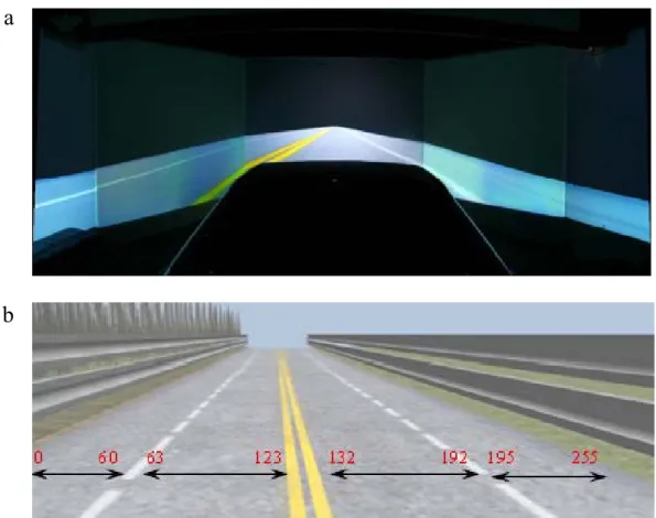
We developed a VR highway environment with a monotonic scene as shown in Fig. 2-4(a) and eliminated all unnecessary visual stimuli. The four lanes from left to right were separated by a median strip in the VR-based scene. The distance from the left side to the right side of the road was equally divided into 256 points for outputting digital signal from WTK program, and the width of each lane and the car was 60 units and 30 units, respectively (as showed in Fig. 2-4(b). In the VR scene, the simulated driving speed was controlled by a scheduled program, thus subjects need not to step on paddles, to prevent large muscle activity on the throttle or brake.

a

b

Fig. 2-4: (a) The photomicrograph showed the simulated high way scene. The monotonous scene was designed to reduce the visual disturbance. (b) The illustration of the high way scene. The width of highway from the left to right side was equally

divided into 256 units and the width of the car was 32 units.

2.3.3 Task Descriptions

Since the main purpose of this dissertation is to investigate distraction effects in dual-task conditions, two tasks involving unexpected car deviations and mathematical questions were designed. In the driving task, the car frequently and randomly drifted from the center of the third lane. Subjects were required to steer the car back to the center of the third lane. This task mimicked the effects of driving on a non-ideal road surface. In the mathematical task, two-digit addition equations were presented to the subjects. The answers were designed to be either valid or invalid. Subjects were asked to press the right or left button on the steering wheel corresponding to on correct or incorrect equations, respectively. The allotment ratio of correct-incorrect equations was 50-50. The choice of mathematic task was motivated by the desire for control in the task demands (Geary and Wiley, 1991). All drivers could perform this mathematic task well without training.

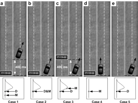
To investigate the effects of SOA between two tasks, the combinations of these two tasks were designed to provide different distracting conditions to the subjects as shown in Fig. 2-5. Five cases were developed to study the interaction of the two tasks. The bottom insets show the onset sequences of two tasks. Therefore, this study investigated the relationship of math task and driving task and how two tasks affected each other in the SOA conditions.

Fig. 2-5: The illustration shows the relationship of occurrences between the deviation and math tasks. D: deviation task onset. M: math task onset. (a) Case 1: math task presents 400ms before the deviation task onset. (b) Case 2: math and deviation tasks occur at the same time. (c) Case 3: math task presents 400ms after the deviation task onset. (d) Case 4: only math task presents. (e) Case 5: only deviation task occurs. The bottom insets show the onset sequences of the two tasks.

2.4 Data Analysis

2.4.1

Behavioral Performance

After recording the behavioral data, statistical package for the social science (SPSS) Version 13.0 for Windows software is applied to estimate the significance testing of behavioral data. The response time of these two tasks (the driving deviation and the math equation) is analyzed to study the behavior of subjects in the experiments.

Using ANOVA (analysis of variance), the significances of the response time of these two tasks are tested for every subject. A non-parametric test is also utilized to study the trends of

the behavioral data. Firstly, this study excluded outliers, comprising around 6.57 % of all trials, based on the criteria that response time was distributed outside the mean response time plus three times the standard deviation of each single session. Secondly, the number of trials in one of five cases which is minimal is chosen to make a benchmark to randomly select the same number of trials in other cases. Thirdly, a single task is taken for the baseline to normalize the behavioral data to be Xi

Xmean (Xi: mean of response time in case i, Xmean: mean of response time in single case). For example, in order to compare the distraction effects from the math equation, case 4 (the single math task) is the baseline.

2.4.2

Distraction Effects of Dual-task

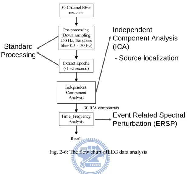
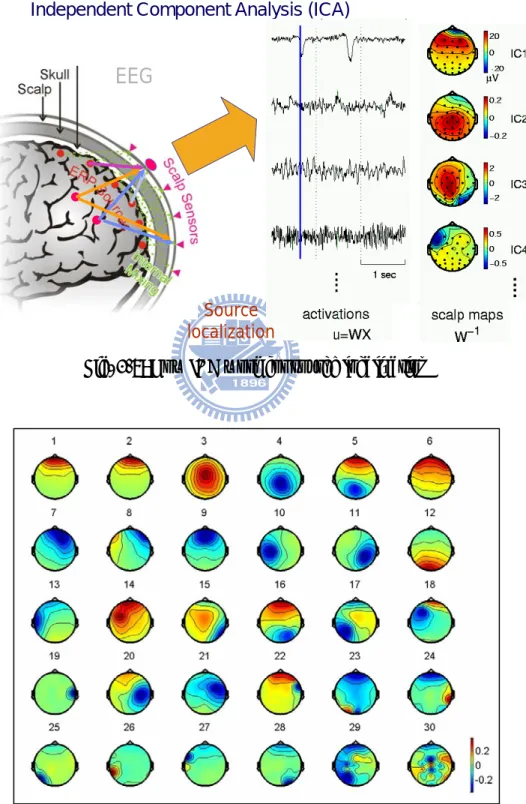
EEG epochs are extracted from the recorded EEG signals with 16-bit quantization, at the sampling rate of 500Hz. The data are then preprocessed using a simple low pass filter with a cut-off frequency of 50 Hz to remove line noise and other high frequency noise. One more high-pass filter with a cut-off frequency of 0.5 Hz is utilized to remove DC drift. This study adopts ICA to separate independent brain sources (Jung et al., 2000; Lee et al., 1999; Makeig et al., 1995). ERSP technology is then applied to these independent component (IC) signals (separated independent brain sources) to transfer the signal into the time-frequency domain for the event-related frequency study. Finally, the stability of component activations and scalp topographies of meaningful components are investigated with component clustering technology. Because different cases with various combinations of driving and the math tasks are designed, EEG responses from five different cases are extracted separately.

Independent

Component Analysis

(ICA)

-

Source localization

Event Related Spectral

Perturbation (ERSP)

Extract Epochs (-1 ~5 second) Independent Component Analysis 30 ICA components Result Pre-processing (Down sampling 250 Hz, Bandpass filter 0.5 ~ 50 Hz) 30 Channel EEG raw data Time_Frequency Analysis

Standard

Processing

Fig. 2-6: The flow chart ofEEG data analysis

EEG source segregation, identification, and localization are very difficult because EEG data collected from the human scalp induce brain activities within a large brain area. Although the conductivity between the skull and brain is different, the spatial “smearing” of EEG data caused by volume conduction does not cause a significant time delay. This suggests that ICA algorithm is suitable for performing blind source separation on EEG data. The first applications of ICA to biomedical time series analysis were presented by Makeig and Inlow (1993). Their report shows segregation of eye movements from brain EEG phenomena, and separates EEG data into constituent components defined by spatial stability and temporal independence. Subsequent technical experiments demonstrated that ICA could also be used to remove artifacts from both continuous and event-related (single-trial) EEG data (Jung et al., 2000; Lee et al., 1999). Presumably, multi-channel EEG recordings are mixtures of underlying brain sources and artificial signals. By assuming that (a) mixing medium is linear

and propagation delays are negligible, (b) the time courses of the sources are independent, and (c) the number of sources is the same as the number of sensors; that is, if there are N sensors, the ICA algorithm can separate N sources (Jung et al., 2000).

‹Independent Component Analysis (ICA)

EEG

EEG

EEG

Source localization

Fig. 2-7: How ICA work for source localization

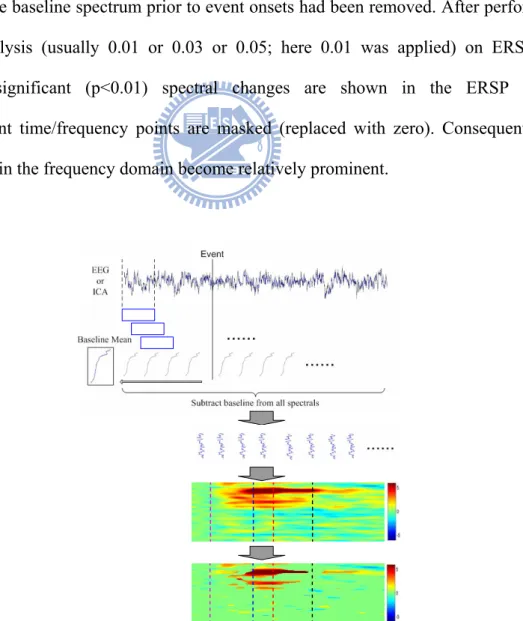
The time sequences of ICA component signals are subjected to Fast Fourier Transform with overlapped moving windows (in Fig. 2-9). In addition, the spectrum in each epoch is smoothed by 3-window (768 points) moving-average to reduce random errors. The spectrum prior to event onsets is considered as the baseline spectrum for every epoch. The mean of the baseline spectrum is subtracted from the power spectral after stimulus onsets so spectral “perturbation” can be visualized. This procedure is then applied repeatedly to every epoch. The results are averaged to yield ERSP images (Makeig, 1993). These measures can evaluate averaged dynamic changes in amplitudes of the broad band EEG spectrum as a function of time following cognitive events. The ERSP images mainly show spectral differences after an event since the baseline spectrum prior to event onsets had been removed. After performing a bootstrap analysis (usually 0.01 or 0.03 or 0.05; here 0.01 was applied) on ERSP, only statistically significant (p<0.01) spectral changes are shown in the ERSP images. Non-significant time/frequency points are masked (replaced with zero). Consequently, any perturbations in the frequency domain become relatively prominent.

window with 256 samples, and there was 244-sample overlap of two adjacent windows. The time-dependent ERSP image was composed of the spectra of each window, and smoothed by 3-window moving average. In the final step, the significant parts of ERSP image were extracted by using bootstrap method. The pink dashed lines: the first event onset. The blue dashed lines: the averaged reaction time to the deviation. The red dashed lines: the averaged response time to math. The black dashed lines: averaged response time for the car returning to the third lane. Color bars showed the magnitude of ERSPs.

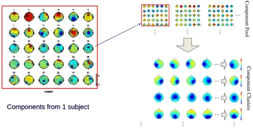
To study the cross-subject component stability of ICA decomposition, components from multiple subjects are clustered, based on their spatial distributions and EEG characteristics. However, components from different subjects differ in many ways such as scalp maps, power spectrum, ERPs and ERSPs. Some studies attempted to solve this problem by calculating similarities among different ICs (Makeig et al., 2002; Makeig et al., 2004; Onton et al., 2005). Based on these studies, ICs of interest are selected and clustered semi-automatically based on their scalp maps, dipole source locations, and within-subject consistency (in Fig. 2-10). To match scalp maps of ICs within and across subjects in this dissertation, the gradients of the IC scalp maps from different sessions of the same subject are computed and grouped together based on the highest correlations of gradients of the common electrodes retained in all sessions. For dipole source locations, DIPFIT2 routines from EEGLAB are used to fit single dipole source models to the remaining IC scalp topographies using a four-shell spherical head model (Oostenveld and Oostendorp, 2002). In the DIPFIT software, the spherical head model is co-registered with an average brain model (Montreal Neurological Institute) and returns approximate Talairach coordinates for each equivalent dipole source.

Components from 1 subject Com pone nt Pool Component Clusters

Components from 1 subject

Com

pone

nt Pool

Component

Clusters

Fig. 2-10: The flowchart of component clustering. Components from all subjects were classified into several significant clusters.

3

Chapter 3

Experimental Results

3.1 Behavioral Performance

To investigate the overall behavioral index, this study uses nonparametric tests because several extremely large scores are significantly skewed. Firstly, the trials of data are randomly selected to have the same number of the trials in all cases. Then, the response time of the deviation and math tasks in the five cases are normalized to correspond to single-deviation and single-math cases, respectively. SPSS software is used for the Friedman test, and the results of which are shown in Fig. 3-1. Dual-task cases are marked for easy discrimination from single-task cases.

Math No rma lized Re s po n se Ti me a b *: p<0.01 D Case 5 M D Case 1 D &M Case 2 D M Case 3 1.2 1.1 1.0 0.9 0.8 M Case 4 M D Case 1 D &M Case 2 D M Case 3 1.2 1.1 1.0 0.9 0.8 Deviation Math No rma lized Re s po n se Ti me a b *: p<0.01 D Case 5 M D Case 1 D &M Case 2 D M Case 3 D Case 5 D Case 5 M D Case 1 M D Case 1 D &M Case 2 D &M Case 2 D M Case 3 D M Case 3 1.2 1.1 1.0 0.9 0.8 M Case 4 M D Case 1 D &M Case 2 D M Case 3 M Case 4 M Case 4 M D Case 1 M D Case 1 D &M Case 2 D &M Case 2 D M Case 3 D M Case 3 1.2 1.1 1.0 0.9 0.8 Deviation

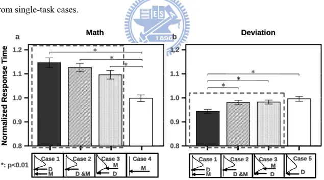
Fig. 3-1: This figure shows the bar charts of normalized response times. (a) for the math task and (b) for deviation task across 15 subjects. The filled black bar: case 1; dark gray bar: case 2; light gray bar: case 3; the open bar: single case. The response time for math task in dual-task cases (case 1, case 2, and case 3) is significantly longer than that for in single task (case 4). The shortest response time for the math

onset is in case 4. The response time for deviation task in case 1 is significantly shorter than those in other cases. The longest response time to the deviation onset is in case 5. The bottom insets show the onset sequences of the two tasks.

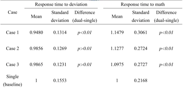
To know how the cases make the differences, the Student-Newman-Keuls test is used for the post hoc test (in Table 3-1). The test statistic on response time of math tasks in cases 1-4, is

χ

2(3)=903.926 from the Friedman’s ANOVA test, and p<0.01. The Student-Newman-Keuls test show three significant groups: case 1 with case 2, case 3, and case 4 in which the response time for math task in case 1 is the longest. Statistical test results of the response time for deviation tasks in cases 1-3, and case 5, is

χ

2(3)=493.98 from the Friedman’s ANOVA test, and p<0.01. Using the Student-Newman-Keuls test, there are two significant groups: case 1, and the other cases in which the response time for deviation task in case 1 is the shortest.

Table 3-1: The normalized response time to deviation and math

3.2 Independent Component Clustering

EEG epochs are extracted from the recorded EEG signals. Then, ICA is utilized to

Response time to deviation Response time to math Case Mean Standard deviation Difference (dual-single) Mean Standard deviation Difference (dual-single) Case 1 0.9480 0.1314 p<0.01 1.1479 0.3061 p<0.01 Case 2 0.9856 0.1269 p>0.01 1.1277 0.2724 p<0.01 Case 3 0.9865 0.1231 p>0.01 1.0975 0.2727 p<0.01 Single (baseline) 1 0.1553 1 0.2168

decompose independent brain sources from the EEG epochs. Based on distraction effects in this study, many brain resources are involved in this experiment. Especially, the motor component is active when subjects are steering the car. At the same time, activations related to attention in the frontal component appear. Therefore, ICA components, including frontal and motor, are selected for IC clustering to analyze cross-subject data based on their EEG characteristics, such as baseline spectrum, Scalp map and Dipole plot.

Based on the baseline spectrum of their EEG characteristics, the baseline spectrums of the same components of different subjects are listed in the Fig. 3-2. The outlier can be observed and removed. In this case (frontal component), green subject is the outlier.

Fig. 3-2: Baseline spectrum of the same components

Then, IC clustering groups massive components from multiple sessions and subjects into several significant clusters. Cluster analysis, k-means, is applied to the normalized scalp topographies and power spectra of all 450 (30 channels x 15 subjects) components from the 15 subjects. Cluster analysis identifies at least 7 component clusters having similar power spectra and scalp projections. These 7 distinct component clusters consisted of frontal, central

midline, parietal, left/right motor and left/right occipital. Table 3-2 gives the number of components in different clusters. This investigation uses the frontal and left motor components to analyze distraction effects. Fig. 3-3 shows the scalp maps and equivalent dipole source locations for fontal and left motor clusters. Based on this finding, the EEG sources of different subjects in the same cluster are from the same physiological component.

Fig. 3-3: The scalp maps and equivalent dipole source locations after IC clustering across 15 subjects. (a) the frontal components and (b) the left motor components are shown in the figure. There are 14 subjects in the frontal cluster and 11 subjects in the left motor cluster. The grand scalp map is the mean of the total component maps in each cluster. The smaller maps are the individual scalp maps. The right panels (c) and (d) show the 3-D dipole source locations (colored spheres) and their projections onto average brain images. The colored source locations correspond to their own scalp maps by the same color of the text above.

Table 3-2: The Number of Components in Different Clusters

3.3 Cluster Analysis

3.3.1

Frontal Cluster

Fig. 3-4a shows the cross-subject averaged ERSP in the frontal cluster corresponding to the five cases. This figure also reveals significant (p<0.01) power increases related to the math task, demonstrating that the power increases in the frontal cluster are related to the math task. The theta power increases in three dual-task cases including cases 1-3 are slightly different from each other. Compared to the single math task (case 4), the power in dual-task cases is stronger. Especially, the power increase in case 1 is the strongest. On the beta band, it also shows power increases, which appear only in the math-task and time-locked to mathematics onsets. Frontal Central Midline Parietal Left Motor Right Motor Left Occipital Right Occipital Number of components 14 7 6 11 6 7 5

Fig. 3-4: The ERSP images of frontal cluster with five cases. (a) The ERSP images of frontal cluster with five cases. The right column show the onset sequences of the two tasks. Color bars indicate the magnitude of ERSPs. Red solid lines show the onset of the math task. Red dashed lines show the mean response time for the math task. Blue solid lines show the onset of the deviation task. Blue dashed lines show the mean response time for the deviation task. The red circle pointed out by the red arrow in case 2 means the red solid line and blue solid line are on the same position. Latencies calculated from (a) are shown in (b) by calculating time form the math task onset to the first occurrence of power increases. The open bars represent the latencies in the theta (4.5~9 Hz) band . The gray bars represent these latencies in the beta (11~15 Hz) band. The comparison of total power in cross-subject (14 subjects) averaged ERSP images in the frontal cluster between cases is shown in (c). The amount of total power

is calculated by adding all the power increases in the same temporal period and the same frequency band. The open bars represent the total power in the theta band. The gray bars represent the total power in the beta band.

In order to find out the suitable and reasonable range of EEG power in Fig. 3-4a, the ranges of frequency are firstly calculated in Fig. 3-5. Then the ranges of the frequency band are defined as “theta band: 4.5 ~ 9Hz” and “beta band: 11 ~ 15Hz”. After defining the ranges of frequency, the ranges of time interval are calculated in Fig. 3-6. Then the ranges of time interval are defined as “theta band: 300~3500 ms” and “beta band: 500~2600 ms”.

Frequency (Hz) Mean p o wer (d B)

Fig. 3-5: Cross-subject ERSP plots for frequency (x-axis)

Time (ms) Be Time (ms) ta band me a n pow er (dB) Theta b a n d me an po w er (dB)

Fig. 3-4b and c give comparisons of the latency and total power in four cases from Fig. 3-4a. It demonstrates that the latencies of power increases in two frequency bands are different with the different SOA time. The shortest latencies in both bands occur in case 1 and the longest power increase latency in the theta band occurs in case 4. It also demonstrates that the amount of power increases in the theta band is different with the different SOA time. The most significant power increase occurs in case 1.

3.3.2

Motor Cluster

Fig. 3-7a shows the cross-subject average ERSP in the left motor cluster corresponding to five cases. Significant (p<0.01) power suppressions appear around the event onsets (at 0ms) and stop at different time axes by cases. In case 4, the alpha and beta power suppressions appear continuously until the red dashed lines, which indicates the mean of the response time for the math task. Compared with case 4, the alpha and beta power suppressions in case 5 are stronger and also last longer. In other cases, the alpha and beta power suppressions continue after the blue dashed lines. This phenomenon is suggested to be related to steering the car back to the center of the third lane.

Fig. 3-7: The ERSP images of the left motor cluster with five cases. (a) The ERSP images of the left motor cluster with five cases. The right column shows the onset sequences of the two tasks. Color bars indicate the magnitude of the ERSPs. Red solid lines show the onset of math. Red dashed lines show the mean response time for math task. Blue solid lines show the onset of deviation task. Blue dashed lines show the mean response time for deviation task. The red circle pointed out by a red arrow in case 2 means the red solid line and blue solid line are on the same position. Latencies calculated from (a) are shown in (b) by calculating from the deviation task onset to the first occurrence of power suppressions. The open bars represent the latencies in the alpha (8~14 Hz) band. The gray blue bars represent these latencies in the beta band (16~20 Hz). (c) shows the comparison of total power in cross-subject (11 subjects) averaged ERSP images in the left motor cluster between cases. The

amount of total power is calculated by adding all the power suppressions in the same temporal period and the same frequency band. The open bars represent the total power in the alpha band. The gray bars represent the total power in the beta band.

In order to find out the suitable and reasonable range of EEG power in Fig. 3-7a, the ranges of frequency are firstly calculated in Fig. 3-8. Then the ranges of the frequency band are defined as “mu suppression: 8 ~ 14Hz” and “beta band: 16 ~ 20Hz”. After defining the ranges of frequency, the ranges of time interval are calculated in Fig. 3-9. Then the ranges of time interval are defined as “mu suppression: 400~3700 ms” and “beta band: 200~3400 ms”.

Frequency (Hz) Mean p o wer (d B)

Fig. 3-8: Cross-subject ERSP plots for frequency (x-axis)

Time (ms) Be Time (ms) ta band me an pow er (dB) Th eta ban d mean p o w er (dB)

Fig. 3-7b and c shows comparisons of the latency and total power between the four cases in Fig. 3-7a. It demonstrates that power suppression latencies in the beta band are different with the different SOA time. The shortest power suppression latency occurs in case 1 and the longest power increase latency occurs in case 5. It also demonstrates that the amount of power suppression in the alpha band is different with the different SOA time. The most significant power suppression occurs in case 5 (the single driving task) and the smallest power suppression occurs in case 4 (the single math task).

3.3.3

Condition Comparison

In order to compare two ERSP in different case, we apply a compared ERSP method with a statistic test in Fig. 3-10. The results will have some black circles with the original ERSP. The areas inside the black circles mean the area with significant power.

Time (ms) F re que ncy (H z) Time (ms)

With significant power inside the black circles

Fig. 3-10: Compared ERSP

significance test. Columns (b) and (e) show the differences among three single-task cases; columns (c) and (f) show the differences between single- and dual- task cases. In columns (b), (c), (e), and (f), a Wilcoxon signed-rank test is used to retain the regions with significant power inside the black circles. Columns (b) and (c) show the comparison of power increases between cases. The remained regions show greater power increases in the single-task case than in the dual-task case. Columns (e) and (f) show compared power suppressions between cases. The remained regions show greater power suppressions in the dual-task cases than in the single-task case.

Fig. 3-11: ERSP without a significance test and the differences between cases. Column (a) shows the ERSP in the frontal cluster without a significance test which

contains all the details of case 1, case 2, case 3, and case 4. Column (b) shows the differences among three single-task cases in column (a). Column (c) shows the differences between single- and dual- task cases in column (a). Column (d) shows the ERSP in the left motor cluster without a significance test which contains all the details of case 1, case 2, case 3, and case 5. Column (e) shows the differences among three single-task cases in column (d). Column (f) shows the differences between single- and dual- task cases in column (d). A Wilcoxon signed-rank test (p<0.01) is used for the statistical test in (b), (c), (e), and (f).

4

Chapter 4

Discussion

The brain dynamics related to distracted effects of stimulus onset asynchrony (SOA) by using EEG and VR-based realistic driving environment was investigated. The SOA experimental design was to investigate the distracted level. In this Chapter, the results after cross-subject analysis would be discussed. Cross-subject analysis was able to prove that the appeared features were not restricted to specific subject or experiment, that was, it could ensure the stability and consistency of pour findings.

4.1 Frontal Cluster

The frontal lobe is an area in the brain, located at the front of each cerebral hemisphere (in Fig. 4-1). The frontal area deals with impulse control, judgment, language production, working memory, motor function, and problem solving (Burgess, 2000; Sarnthein et al., 1998). In Fig. 3-4a, the greater frontal power increases in cases 1-4 appear due to the solving of the math questions. The power increases in the theta (4.5~9 Hz) and beta bands (11~15Hz) appear briefly after the math onset. Fig. 3-4b and c show the quantified frontal power latencies and power increases in four conditions for the purpose of discussing the EEG dynamics made by solving the math question. In the theta power, the shortest latency is revealed in case 1. Power increases in three dual-task cases are higher than that in single-task case with the greatest power occurring in case 1. These phenomena suggest that dual tasks induce more event-related theta activities as well as subjects need more brain resources to accomplish dual tasks. The theta increase is associated with numerous processes such as mental work load, problem solving, encoding, or self monitoring (Onton et al., 2005). Based on this evidence, the study demonstrates that the subjects were distracted under dual-task conditions in the

experiment.

Fig. 4-1: Picture showed the principle fissures and lobes cerebrum (Kandel et al.) The blue part is the frontal lobe and the white area is the location of parietal lobe.

Since human visual sensors need about 300 ms to induce event-related potential (P300 activity, Jensen et al., 2001), we have also tested several kind of intervals between first and second task, 400 ms between twso tasks is sufficient for a subject to perceive stimulus. In case 1, a processing task is already in the brain and subjects need more brain resources to manage the high priority task presented 400 ms after the processing task. Therefore, the total power in the theta band in case 1 is the highest as shown in Fig. 3-4c. Clearly the theta power increase appears the earliest in case 1 as shown in Fig. 3-4b. The early theta response in the frontal area primarily reflects the activation of neural networks involved in allocating attention related to the target stimulus (Missonnier et al., 2006).

The trends of response time for the math task (in Fig. 3-1a) and EEG theta increases in the frontal cluster (in Fig. 3-4c) are consistent with one another (in Fig. 4-2). In the case of the single math task, the response time is the shortest and the theta power increase is the weakest. Among the dual-task cases, the longest response time and the greatest theta power increase

are in case 1. This evidence suggests that the theta activity of the EEG in the frontal area during dual tasks is related to distraction effects and represents the strength of distraction. In addition, power increases in the beta band appear in all cases. From the ERSP images, the patterns are time-locked to the onset of the math task. Fernández et al. (1995) suggested that significant EEG beta band differences in the frontal area are due to a specific component of mental calculation. 2.5 1.5 0 Power (dB) x103 1.0 0.5 2.0 M Case 4 M D Case 1 D &M Case 2 D M Case 3 2.5 1.5 0 Power (dB) x103 1.0 0.5 2.0 M Case 4 M D Case 1 D &M Case 2 D M Case 3 M Case 4 M Case 4 M D Case 1 M D Case 1 D &M Case 2 D &M Case 2 D M Case 3 D M Case 3 RT of Math N o rm al iz ed Re s p o n se T im e M Case 4 M D Case 1 D &M Case 2 D M Case 3 1.2 1.1 1.0 0.9 0.8 Behavior performance RT of Math N o rm al iz ed Re s p o n se T im e M Case 4 M D Case 1 D &M Case 2 D M Case 3 1.2 1.1 1.0 0.9 0.8 RT of Math N o rm al iz ed Re s p o n se T im e M Case 4 M D Case 1 D &M Case 2 D M Case 3 M Case 4 M Case 4 M D Case 1 M D Case 1 D &M Case 2 D &M Case 2 D M Case 3 D M Case 3 1.2 1.1 1.0 0.9 0.8 Behavior performance EEG Power 4.5~9Hz 11~15Hz M Case 4 M D Case 1 D &M Case 2 D M Case 3 M Case 4 M Case 4 M D Case 1 M D Case 1 D &M Case 2 D &M Case 2 D M Case 3 D M Case 3 RT of Math Normal ized Re s ponse T ime M Case 4 M D Case 1 D &M Case 2 D M Case 3 1.2 1.1 1.0 0.9 0.8 Behavior performance RT of Math Normal ized Re s ponse T ime M Case 4 M D Case 1 D &M Case 2 D M Case 3 1.2 1.1 1.0 0.9 0.8 RT of Math Normal ized Re s ponse T ime M Case 4 M D Case 1 D &M Case 2 D M Case 3 M Case 4 M Case 4 M D Case 1 M D Case 1 D &M Case 2 D &M Case 2 D M Case 3 D M Case 3 1.2 1.1 1.0 0.9 0.8 Behavior performance EEG Power 4.5~9Hz 11~15Hz 0 0.5 1.0 1.5 Lat e n c y ( sec)

Fig. 4-2: The trends of response time for the math task and EEG theta increases in the frontal cluster are consistent with one another.

4.2 Motor Cluster

Mu rhythm (μ rhythm) is an EEG rhythm usually recorded from the motor cortex of the dominant hemisphere. It can be suppressed by simple motor activities such as clenching the fist of the contra lateral side, or passively moved (Kuhlman, 1978a; Kuhlman, 1978b; Schoppenhorst et al., 1980). Mu suppression is believed to be the electrical output of the synchronization on large portions of pyramidal neurons in the motor cortex that controls hand and arm movements.

In this study, the mu suppressions (8~14 Hz) and beta power suppression (16~20Hz) are mostly caused by subjects steering the wheel and pressing buttons as shown in Fig. 3-7a. The mu suppressions caused by steering the wheel are almost time-locked to the response onset of driving task in cases 1-3 and case 5. However, the mu suppressions caused by pressing the buttons have no effects in case 4. As for in the dual-task cases, the mu suppressions are weaker than those in single-task case. This may due to the competition of brain resources required by wheel steering and button pressing.

Thus, Fig. 3-7b and Fig. 3-7c show motor power latencies and power increases in 4 cases for the purposes of discussing the EEG dynamics caused by the driving task. In (b), the longest latency of beta power suppression is observed in case 5 and the shortest latency appears in case 1. Perhaps motor planning is involved in preparing for steering the wheel and answering the math questions (Hayhoe et al., 2003). In (c), the three dual-task power suppressions are weaker than those in single task. Based on above evidences, it suggests that math processing occupies more brain resources in the frontal area during dual-task cases so less activation is induced in the motor area.

4.3 Other Clusters

To study the cross-subject component stability of ICA decomposition, components from multiple sessions and subjects were clustered based on their spatial distributions and EEG characteristics. Component clustering grouped massive components from multiple sessions and subjects into several significant clusters. Cluster analysis, k-means, applied to the normalized scalp topographies and power spectra of all 450 (30 channels x 15 subjects) components from the 15 subjects, and identified at least 7 clusters of components having similar power spectra and scalp projections.

These component clusters also showed functionally distinct activity patterns. Five other distinct component clusters (as shown in Fig. 4-3) accounted for central midline, parietal, right motor and left/right occipital, respectively. These were effectively removed from the activity of the other component clusters by the ICA decomposition and are not further considered here. The numbers of components in different clusters were given in Table 3-2.

occipital (D) and the right occipital (E) clusters across 15 subjects. Upper panels: the grand mean of the component map. Lower panels: individual scalp maps for the corresponded IC cluster.

4.4 More Behavioral Experiment

In order to have more powerful result, the number of subject should be more. Due to the original number is 15 and the behavioral results don’t have enough significant difference, we invited more subjects to participate this experiment with only behavioral response recorded.

4.4.1

Subjects

The total number of volunteer subjects was 25 in this study. The mean age of subjects was 26.2 years, and the standard deviation of age was 2.9 years. All subjects owned a valid driving license and had a mean reported driving experience of 5 years. All subjects were free of neurological and psychological disorders, as well as drug and alcohol abuse. Experimental procedures were approved by the Institutional Review Board of Taipei Veterans General Hospital.

4.4.2

Experiment Results

The mean and the standard deviation of RT in the four different conditions were listed in Table 4-1. In responding the car deviation task, the mean RT of single-task condition was the longest (656.2 ms). In answering the math equation task, the mean RT of single-task condition was 1700.9 ms and was clearly shorter than other conditions. In comparison with RTs of responding the car deviation and answering the

math equation in single-task conditions, subjects used more resources and took more time on answering the math equation which showed that answering the math equation task could be as a distracting factor because its difficulty was harder than responding the car deviation task.

Table 4-1: Summary data for responding car deviation and answering math equations variable across all trials (2187 trials for each condition), mean response time (Mean, in milliseconds), standard deviation (SD) and accuracy rate (AR).

Types Mean SD AR

(%) ponding the car deviation

Dual-task condition

?400 ms SOA (math first and then deviation onset) 627.9 108.0 － 0 ms SOA (math and deviation occurred simultaneously) 650.5 115.3 － 400 ms SOA (deviation onset first then math) 648.0 114.1 － Single-task condition

Only car deviation 656.2 130.5 －

wering the math equation Dual-task condition

?400 ms SOA (math first and then deviation onset) 1972.2 673.9 94.6 0 ms SOA (math and deviation occurred simultaneously) 1943.5 633.4 94.1 400 ms SOA (deviation onset first then math) 1852.4 592.0 93.9 Single-task condition

Only the math equation 1700.9 468.5 94.6

Fig. 4-4a and Fig. 4-4b how the bar chart of the mean and the standard deviation of RT in responding the car deviation task and answering the math equation task, respectively. In responding the car deviation task, the mean RT under the −400ms SOA condition (mean RT equals 627.9ms) was significantly shorter than the other three conditions (mean RT range was

from 648.0 to 656.2 ms) according to the repeated measures ANOVA (F3,2186 = 75.64, p < 0.01) statistics test. Specifically, the mean RT in the single-task condition was longer than that in dual-task conditions. In answering the math equation task, the mean RT in the −400ms SOA condition (mean RT = 1972.2ms) were longer than the other three conditions (mean RT range, 1943.5 to 1700.9ms) according to the repeated measures ANOVA (F3,2186 = 257.63, p < 0.01) statistics test. Specifically, the mean RT in the single-task condition was significantly shorter than that in dual-task conditions.

In addition, overall accuracy of answering math equations was over 94%. There were no significant effects within three dual-task conditions (χ2(3) = 1.837, p > 0.01).

b

a

Fig. 4-4: Statistical significance of the dual tasks in each condition was analyzed by repeated measures ANOVA followed by pair wise comparisons. Error bar indicates ± 1．SE. Panel (a) shows mean response time for responding car deviation. The repeated measures ANOVA test reveals RT of －400ms SOA condition was significantly lower than those in other conditions. Panel (b) shows mean response time for answering math questions. The repeated measures ANOVA test results show that RT in the － 400ms SOA condition was significantly higher than those in other conditions except in the 0ms SOA condition.