Colored timed Petri net based statistical process control and fault diagnosis to flexible manufacturing systems

Proceedings of the 1997 EEE

International Conference on Robotics and Automation Albuquerque, New Mexico - April 1997

COLORED TIMED PETRI NET BASED STATISTICAL PROCESS CONTROL AND FAULT

DIAGNOSIS TO FLEXIBLE MANUFACTURING SYSTEMS

Chung-Hseng Kuo

*,

Robotics Laboratory, Department of Mechanical Engineering National Taiwan University, Taipei, TAIWAN 10674, R.O.C.

e-mail: hphuangBw3 .me.ntu.edu.tw TEL/FAX: (8 86)2-3 63 3 875

“Professor and correspondence addressee *Graduate student

Abstract

The quality consistence and machines’ utilization of a flexible manufacturing system (FMS) strongly depend on the statistical process control (SPC) and the correct fault diagnosis of equipments. An FMS can be modeled by the Colored Timed Petri Net (CTPN). However, the CTPN models of most FMSs lack the activities of the statistical process control (SPC) and fault diagnosis, and they lead to the incomplete FMSs’ CTPN models. In this paper, the CTPN-based SPC and fault diagnosis models are proposed to model the FMSs’ SPC and fault diagnosis behaviors. Since the models depend on the measured data from the inspection machines and the sensors’ data from the devices, the CTPN-based SPC and fault diagnosis models can be incorporated into the production CTPN models to give a complete model of FMSs’ activities. It will be shown the CTPN-based fault diagnosis is easy to model, and the results are straightforward.

Introduction

A flexible manufacturing system (FMS) is usually efficient and flexible since it combines both the efficiency of flow shop production and flexibility of job shop production. The performance of an FMS relies on the correct system model and analysis. The quality consistence and machines’ utilization are very important to the FMS, and they strongly depend on the statistical

process control (SPC) and the correct fault diagnosis of

devices. Thus, it is necessary to include the SPC and fault diagnosis activities in the FMS model. Petri net is a convenient tool to model and analyze the FMSs. However, most Petri net models to the FMS [3-5, 10,12-141 focus on the production model. Those models are incomplete due to the lack of the statistical process control (SPC) and fault diagnosis activities. In this paper, the CTPN (colored timed Petri net)-based SPC and fault diagnosis are proposed to compensate the incompleteness of the CTPN model of the FMS.

The proposed CTPN model is described in the modular, object-oriented and hierarchical manner, and the FMS under study is a hierarchical structure. Such a configuration is easy to model because of the modular and hierarchical properties. The activities in an FMS are

imbedded in multi-level structures [3, 8, 10, 13, 141; i.e.,

production, process, cell and machine levels. The hierarchical and modular properties of the FMS will be

characterized by the macro transitions and

communication places. Based on the knowledge of FMS

and CTPN, the CTPN model of the FMS is also divided into production, process, cell and machine levels.

The break-down and maintenance of machines are modeled in the machine layer. In this study, the sensor- based CTPN is used to model the fault tree for analyzing the Failure Modes and Effects Analysis (FMEA). The sensor-based CTPN can be used to model the fault diagnosis for identifying the failure equipments (components, machines or cells). Once the FMS is break- down, the CTPN based diagnosis can conclude one or more defect cells. If one cell is found to be break-down, the CTPN based diagnosis can conclude one or more defect machines. If one machine is found to be break- down, the CTPN based diagnosis can conclude one or more defect equipments. On the other hand, the statistical process control (SPC) is a common tool to analyze the cause effect of the product’s defect and ensure the product’s quality. In this manner, the CTPN can be used to model the behavior of the statistical process control in order to include the SPC activities in the FMS!;’ model. Since the CTPN-based SPC and fault diagnosis models depend on the measured data from the inspection machines and the sensors’ data from the devices, they can be incorporated into the production CTPN models to give a complete model of FMSs’ activities. Finally, the proposed CTPN models are applied to the FMS at the Department of Mechanical Engineering, National Taiwan University. In this real-time FMS simulator, thirteen dispatching rules are adopted to operate this FMS simulator, and these dispatching rules can be machine or workpiece dependent. This real-time FMS simulator is developed on a real-time object-oriented expert system G2 [2].

Flexible Manufacturing Systems

An FMS typically consists of a number of sub-

production systems, such as process actions, material handling devices, material storage, control units, inspection station and gauging stations. The flexible manufacturing cells, machines and equipments are often connected through an automated material delivery system.

Production control messages including process

information, product information and control commands

are routed via a communication system. The

communication system consists of computers, control units and a local area network (LAN). FMSs inherit the advantages of high flexibility of the job shop production and the high efficiency of the flow shop production. Thus, FMSs can achieve the purpose of production with multiple types and low quantity.

Functionally, the FMS can be decomposed into the

following four levels [ l , 8, 141. They are ( 1 ) Production

level: this is the highest level in an FMS. It handles the operations of the system including: master production

schedule (MPS), system resource management, database,

maintenance schedule and system performance

measurement. (2) Process level: it coordinates and controls all of the cells in FMSs. For example, the function of real-time scheduling (dispatching) is in this level. (3) Cell level: It is the level of the manufacturing cells below the process level. (4) Machine level: It may be the machining, inspection and material handling equipments such as conveyors, machining center, lathe machine, milling machine, inspection center, robot and automated guide vehicle (AGV).

Colored Timed Petri Net (CTPN)

The CTPN extends the framework of the original PN by adding color and time attributes to the net. The

color attribute [3, 4, 5 , 8, 91 is developed to tackle large

systems that have many similar or redundant logical structures. The time attribute [3, 4, 8, 91 allows various time-based performance measures to be conducted in the system model. A time-delay can be assigned to either places or transitions to model the time elements in a system.

In an PN, when a token in an immediate place is enabled, the condition of the output transition determines the fate of the token. If the output transition is an immediate transition then the token that is enabled fires and escapes from the input place. In the meantime, the transition releases this token to the output place(s). On the other hand, if the output transition is a timed transition, then the token will not be fired until a prescribed time delay is reached. Tokens in a timed place are processed in a similar way.

Notice that the number of arcs between the input place(s) and the output transition(s) is also important to the token. Three types of arcs are used; namely, directed, inhibitor and interrupt arcs. The directed arc connects between a place and a transition, or vice versa. It has no preconditions associated with it. The inhibitor and interrupt arcs are defined as follows. The place connected with the inhibitor arc is called the inhibitor place. When the inhibitor place contains the same color token as the output transition, then the output transition is inhibited to fire. Similarly, the place connected with the interrupt arc is called the interrupt place. When the interrupt place contains the same color token as the output transition, then the firing in the output transition is interrupted and further inhibited. For the immediate transition case, the interrupt and the inhibitor arcs behave the same. For the timed transition case, the interrupt and the inhibitor arcs do not behave the same. If the timed transition is firing and the interrupt place has the same color, then it interrupts the firing of this transition and returns the color

token to the input place(s) [4, 8 , 9 , 13, 141.

Modular design [lo] is essential for a compact FMS model. In addition to the four levels mentioned above, each level is broken down into several sub-systems in the similar fashion. For example, the cell level under

study consists of a FMCl and FMC2. To facilitate a

modular design, individual modules are developed first for each of the four levels. Then, the modules of different levels are integrated together to form the complete FMS model.

In this approach, macro transitions are often used

to formalize a modular design [3, 4, 8, 9, 12, 13, 141. A

macro transition is the combination of a series of transitions, places and arcs. A macro transition may consist of several sub-macro transitions (it is, in essence, a macro transition but in different levels). A system can

be composed of many macro transitions. The

interconnection between different levels is achieved by communication places. Based on macro transitions and communication places, a hierarchical and modular model of the FMS can be constructed.

The communication and interface between the

macro transitions are through four types of

communication places, and they are pitch-up, pitch-down, catch-up and catch-down places. The pitch-down and catch-down places are applied to the higher level modules, and the pitch-up and catch-up places are for the lower level modules. The higher level modules use the pitch- down place to send (or pitch) tokens to the lower level modules, and use the catch-down place to receive (or catch) tokens from the lower level modules. Similarly, the lower level modules use the pitch-up place to send tokens to the higher level modules, and use the catch-up place to

catch tokens from the higher level modules [4, 8, 9, 13,

141.

In the framework of the hierarchical design, we

can model an FMS modularly. The primary

considerations are to make the model easy to extend, maintain and debug in the future. The icon definition of CTPN is shown in Fig. 1.

Modeling an FMS by Using CTPN

The structure of the FMS is decomposed into four

hierarchical levels. The CTPN model is built in the

manner of modular design. Each module of the CTPN model is based on macro transition. The material flow and information flow in the FMS are integrated by the communication places. The following notions are used in the modeling of an FMS:

1. Immediate place describes the resources of the FMS

such as material, machine, message, control command and buffer.

2. Timed place is used to model a place that is associated with a time-delay, e.g. a conveyor belt

on which components stay for a certain time.

3. Communication place describes a place which

provides communication between macro transitions, such as that between a cell layer and a machine layer.

4. Immediate transition models the event occurred in the FMS, e.g. a machine completes one job. On the other hand, it can also model a decision making,

such as selecting the next product type for a

machine under a specific dispatching rule.

5. A timed transition can describe a process that needs time to complete.

6 . Macro transition models the aggregation of many process such as the cells or machines.

CTPN for Maintenance, Diagnosis and SPC

Maintenance, fault diagnosis and statistical process control (SPC) play very important roles for the FMSs’ performance. They affect the machine utility, system performance and quality control directly. In this section,

the CTPN model is further applied to the modeling of the activities of SPC, fault diagnosis of machines and equipment maintenance in FMSs

-

-

-

Figure 1. Icon definition of CTPN graph. The sensor based CTPN is used to model the fault tree and analyze the Failure Modes and Effects Analysis (FMEA). Similarly, the CTPN-based fault diagnosis is developed to identify the failure equipments (components, machines or cells). Finally, the CTPN is used to model the behaviors of statistical process control (SPC) in FMSs.

Machines or equipments can not work when they are broken or being maintained. Thus, the fault diagnosis and maintenance of machines must be included in the CTPN model. The activities of fault analysis and maintenance of machines are modeled in the CTPN

machine level. Fig. 2 shows the details (the right hand

side of that net).

... ... ... . .... ... ... .. . ... ... ... ... .. .. (7J[q-"

: ULhr. .K."".IM..ma,"x *u*l

Figure 2. Modeling the machine fault and maintenance. Fault tree is a common and convenient method to analyze the failure modes and effects, and it can identify the various possible failure modes and effects. The fault tree analysis aims at developing the structure from which simple logic relationships can be used to express the probabilistic relationships among the various events that lead to the failure of the system. In this paper, the FMEA and fault diagnosis are both considered for the FMSs. The sensor based CTPN is developed to model the FMEA from the fault tree, and to model the fault diagnosis to identify the broken equipments [ 81.

In a factory, every sensor has its corresponding components. For example, level gauge is corresponding to the tank, and pressure gauge is corresponding to the pump. Thus, a sensor based configuration is used to construct the fault tree. The events are defined as follows:

(1) On-off sensors, by traditional PN. ( 2 ) Analog sensors,

divide the analog sensor value into appropriate levels. For example, the value of level gauge can be classified into the HiHigh, High, Normal, Low, LoLow levels.

Based on the hierarchical and modular

configuration, the CTPN is used to construct the fault tree

hierarchically. The CTPN elements such as places and

transitions can map with the fault tree elements. Some important fault tree symbols that relate to the FMS are

selected, such as AND gate, OR gate, condition gate,

order AND gate, basic events, intermediate events and transfer events. The transformation is described as follows: (1) Events, modeled by places. ( 2 ) Gates, modeled by transitions. (3) Composite systems, such as FMS, modeled by hierarchical and modular configuration. Fig.3 shows the transformations between the CTPN and the fault tree for the failure modes and effects application. In Fig.3, A, B and C are sensor recordings; T is the event; SI, S2, S3, S4 are the message communication places. Fig.4 shows the transformations between the CTPN and fault tree for the fault diagnosis application. In Fig.4, A, B and C are sensor recordings; T

is the event; EA, EB and EC are the diagnosis results, and

they are corresponding to the sensors A, B and C. In addition, Fig.5 shows an example of the fault tree application. Fig.6 and Fig.7 are the corresponding relationships to the fault tree example in Fig.5.

In order to achieve high and stable quality, the

automated inspection unit is necessary in FMS. SPC [6,

1 I ] is a common method to determine whether a process

is in control or out of control. In other words, SPC can identify the assignable causes, adjust the process and eliminate the process variance. In addition, process capability analysis is a key point to prevent defects from occurring. Although the FMS is capable of small batch production, the specifications of different products or even the same product but with small quantity can not be used in the statistical application. Thus, it is necessary to modify the specifications among different products. A scaled variable is used here to normalize the specification among different product so that they can be discussed and analyzed on the same control chart [7]. The output scaled variabley is defined as

where x is the measured data, and a and b are scale

factors.

In this paper, seven SPC tools are constructed to analyze the process. The seven SPC tools are: histogram, check sheet, Pareto chart, cause and effect diagram (C-E diagram), defect concentration diagram, scatter diagram, and control chart. The SPC activities in the FMS can be analyzed in Fig.8. The CTPN model of SPC activities is constructed in Fig. 9.

Clearly, the sensor-based CTPN can be used to model the fault diagnosis for identifying the failure equipments (components, machines or cells). Once the FMS is breakdown, the CTPN-based diagnosis can conclude one or more defect cells. If one cell is found to be breakdown, the CTPN based diagnosis can conclude one or more defect machines. If one machine is found to be break-down, the CTPN based diagnosis can conclude one or more defect equipments. In addition, the cause effect of the product's defect and the product's quality can be analyzed by the CTPN-based model of SPC. Since the CTPN-based SPC and fault diagnosis models depend on the measured data from the inspection machines and the sensors' data from the devices, they can be incorporated into the production CTPN models to give a

complete model of FMSs' activities.

An Application Example

x - U ,

y = -

The proposed CTPN modeling technique is applied to an FMS example. This example illustrates how

can one create

a

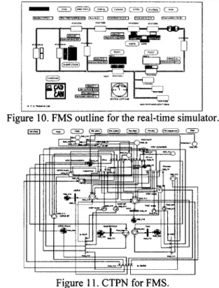
implement this CTPN model into a real-time FMS simulator. Besides, thirteen dispatching rules are used to operate this FMS real-time simulator. The FMS case under study is an experimental automated factory in the Department of Mechanical Engineering, National Taiwan University. It includes a transportation cell, a storage cell, two FMCs and one inspection cell. The layout of the corresponding FMS simulator is given in Fig. 10.

,.,*No#". *,"a*

8

Figure 3. Transformation between CTPN and fault tree for the failure modes and effects application.

<.1U"l. , b ) o L b u

Figure 4. The transformation between CTPN and fault tree

for the fault diagnosis application.

w w

Figure 5. An example of fault tree application.

Figure 6 . The corresponding relationships to the fault tree

example in Figure 5 for the FMEA analysis. This simulator has to be operated by using some efficient dispatching rules. Thirteen dispatching rules [S,

141 are developed in terms of workpiece characteristics and machine characteristics as follows. They are first come first serve (FCFS), shortest processing time (SPT), weighted shortest processing time (WSPT), shortest remaining processing time (SRPT), longest remaining processing time (LRPT), fewest operation remaining time (FORT), largest operation remaining time (LOW),

earliest due date (EDD), shortest operation time with

alternative considered (SOTA), earliest starting time with alternative considered (ESTA), longest idle time with alternative considered (LITA), earliest finishing time with alternative considered (EFTA) and combination of "LITA" and "ESTA" ("LITA"

+

Figure 7. The corresponding relationships to the fault tree example in Figure 5 for the fault diagnosis.

,

Figure 8. The application of SPC activities in FMS.

Figure 9. Model SPC by using CTPN.

The complete FMS model can be constructed by using CTPN. In the system level, there is a CTPN net for

FMS, and Fig. 11 shows the details. In the cell level, there

are CTPN nets for FMC1, FMC2, AGV, AS/ RS and

inspection cells.

Since there are too many data from real-time simulator, only part of results are presented here. Table 1 shows the batch data setting for this simulation, and there is only one workpiece for each batch. The setup data provides the initial conditions of FMS production. Table 2 shows the simulation results under different dispatching rules, and it also indicates the time needed for different dispatching rules to operation. In addition, the number of

system bottle neck index and the order of every workpiece that completes all processes under different dispatching rules are also discussed. The system bottle neck index is the risk of the system to occur bottle neck under one specified dispatching rule. This index is measured from the simulation results and it represents the frequency of the system to be in the bottle neck conditions.

R u l e S e t u p C o m p l e t e P r o c e s s i n g

T i m e T i m e T i m e

I I I I -.*

Figure 1 1. CTPN for FMS.

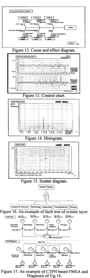
The SPC on-line query displays are also provided. Fig.12 shows the cause and effect diagram. It is an important function of SPC. Fig. 13 shows the control chart. In this figure, one can judge whether the process is in control or out of control. Fig. 14 shows the histogram for a measured data. Generally, the distribution of the measured data is a normal distribution. Fig.15 shows the scatter diagram. One can discuss the relationship between two measured data, and the results can be used to improve the process. Besides, process capability analysis and Pareto chart are also provided, but they are not included in this paper.

The CTPN-based fault diagnosis is a multi-layer configurations. Fig.16 shows the fault tree of the system layer. The corresponding FMEA analysis and fault diagnosis CTPN net is shown in Fig.17. REL-FMSP1 to REL-FMS-P5 are the status collected from the cell layer. If there exists one token in REL-FMS place, then this FMS will break down. DIAG-FMS-PI, DIAG-FMS-P3,

DIAG-FMS-P5, DIAG-FMSP7, DIAG-FMS-P9 are

the status collected from the cell layer. If there is one token in DIAG-FMS place, then there must be at least one cell in trouble.

Conclusions

In this paper, the integrated CTPN environment is constructed to model the activities occurred in the FMS. Not only the production activities but also the SPC,

B o t t l e N e c k I n d e x . SPT 149 s e c C o m p l e t e S e q u e n c e W S P T 1139 s e c C o m p l e t e S e q u e n c e S R P T 1109 s e c C o m o l e t e S e a u e n c e F C F S 1634 s e c 16159 s e c 15525 s e c l n o n e

I

I

Table 2. Some simulation results under different dispatching rules.

C."_

-

B).

Figure 12. Cause and effect diagram.

I

Figure 13. Control chart.

I

I

I I

Figure 14. Histogram.

__1__________^_ E

Figure 15. Scatter diagram.

Figure 16. An example of fault tree of system layer.

Figure 17. An example of CTPN based FMEA and

Diagnosis of Fig. 16.

Acknowledgment

This work was partially supported by the National Science Council, Taiwan, R.O.C., under Grant NSC85- 22 12-E-002-073, and NSC85-2622-E-002-018

References

A. Bauer, R. Bowden, J. Browse, J. Duggan and G.

Lyons, Shop Floor Control System -@om Design to

Implementation , London: Chapman & Hall, 199 1.

G2 Reference Manual Version 4.0

,

H.P. Huang and P.C. Chang, "Specification, Modeling and Control of a Flexible Manufacturing

Cell," Int. J. Production Research, Vol. 30, No. 11,

H.P. Huang and Y.H. Tseng, "Modeling and

Graphic Simulator for Integrated Manufacturing

Systems," Intelligent Automation and

Soft

Computing, Vol. 1, pp. 183-186, 1994.

P. Huber, K. Jensen and R.M. Shapiro, "Hierarchies in Coloured Petri Nets," Advanced in Petri Nets

1990, Lecture Notes in Computer Science,

Springer-Verlag, pp. 313-341, 1990.

G.B. Hutchins, Introduction to Qualiq,

Management, Assurance and Control, New York:

Maxwell Macmillan International Publishing

Group, 199 1.

D.L. Kimbler and B.A. Sudduth, "Using Statistical Process Control with Mixed Parts in FMS," JAPAN/ USA Symp. on Flexible Automation, Vol.

C.H. Kuo, "Application of Reliability and

Equipment Maintenance to Flexible Manufacturing

Systems," Master Thesis, Department of

Mechanical Engineering, National Taiwan

University, 1995.

C.H. Kuo and H.P. Huang, "Dispatching and Simulation for Highly Model-Mixed Automotive

Plants," Proc. Int. Conference on Automation

Technology, Taiwan, Vol. 1, pp. 423-430, 1996. pp. 2515-2543, 1992.

1, pp. 441-445, ASME 1992.

[lo] S.S. Lu and H.P. Huang, "Modularization and Properties of Flexible Manufacturing Systems," in

Advances in Factories of the Future, CIM and

Robotics (edited by M. Cotsaftis and F. Vemadat), Amsterdam: Elsevier, pp. 289-298, 1993.

[ 1 I] D.C. Montgomery, Introduction to Statistical Quality

Control , second ed. , New York: John Wiley &

Sons Inc., 1990.

[I21 C.J. Tsai and L.C. Fu, "Modular Approach for Petri- Nets Modeling of Flexible Manufacturing Systems Adaptable to Various Task-Flow Requirement,"

Proc. IEEE Int. Con$ on Robotics and Automation,

France, pp. 1043-1048, 1992.

[ 131 Y.H. Tseng, "Modularized Modeling and Simulation of a Flexible Manufacturing System," Master Thesis, Department of Mechanical Engineering, National Taiwan University, 1993.

E141 M.C. Yeh, "Development of Shop Floor Control System for flexible Manufacturing Systems,"

Master Thesis, Department of Mechanical