行政院國家科學委員會專題研究計畫 成果報告
晶圓製造廠非穩態環境下之生產排程規劃與系統綜合績效
評估(3/3)
計畫類別: 個別型計畫
計畫編號: NSC93-2213-E-009-017-
執行期間: 93 年 08 月 01 日至 94 年 07 月 31 日
執行單位: 國立交通大學工業工程與管理學系(所)
計畫主持人: 鍾淑馨
計畫參與人員: 李欣怡、賴志偉、范國基、高清貴
報告類型: 完整報告
處理方式: 本計畫可公開查詢
中 華 民 國 94 年 7 月 27 日
行政院國家科學委員會專題研究計劃成果報告
晶圓製造廠非穩態環境下之 生產排程規劃與系統綜合績效評估 (3/3)
Production Schedule Planning and Synthetic Performance Evaluation of Wafer Fabs under a Non-Steady State Environment (3/3)
計畫編號:NSC 93-2213-E-009-017 執行期限:93 年 08 月 01 日至 94 年 07 月 31 日 計畫主持人:鍾淑馨 交通大學工業工程與管理學系教授 計畫參與人員:李欣怡、賴志偉、范國基、高清貴 中文摘要 在競爭激烈的市場環境下,公司必須有效地利用產能,以獲取較高的利潤。本計畫的目的為發 展一套能找出一組最適產品(族)組合的有效方法,使公司不論在單期或是多期下營運都能最佳化 生產。本計畫使用模擬模式來蒐集半導體廠不同的產品組合下的績效資料。在單期環境下,由於資 料包絡法對投入項與產出項不需事先給予權重,吾人因而用其來比較各組產品組合之效率,以獲得 每一產品組合相對其他產品組合的效率值。而對於半導體廠隨著期別不同而產出量改變的情況,為 了確保長期的生產績效和利潤獲取,因此選用資料包絡法的視窗分析,來找出連續多期營運下,最 被建議的一組產品族組合。利用此方法,每一產品組合之績效不僅與同期其他產品組合比例之績效 來相比,也跟不同時期同一產品組合之績效來相比。本計畫所提出之方法,可提供晶圓廠有關主生 產規劃的參考,用以改善半導體廠的效率。 關鍵字:資料包絡分析法、產品組合、產品族組合、視窗分析、績效衡量 ABSTRACT
In a competitive market, a company needs to effectively utilize its current capacity in order to acquire higher profit. The purpose of this project is to present an effective approach to find a set of product (family) mix for the company to achieve the optimal production both in a single period and in multiple periods. Simulation is first used to generate the data of performance measures of different product mixes in a semiconductor fabricator. For a single period, data envelopment analysis (DEA) is applied to measure multiple inputs and outputs, without pre-assigning weights, for product mixes, and an efficiency score for producing each product mix relative to other mixes can be obtained. To ensure long-term effectiveness in productivity and in profit gaining, DEA window analysis is adopted for multiple periods to seek the most recommended set of product family mixes for manufacturing by measuring the performance changes over time. With this method, the performance of a mix in one period is compared not only with the performance of other mixes but also with its own performance in other periods. The proposed models
can provide guidance to wafer fabs regarding strategies for aggregate planning so as to improve manufacturing efficiency.
Keywords: Data envelopment analysis, product mix, product family mix, window analysis, performance
evaluation.
1. Introduction
Today’s semiconductor market is not as prosperous as it was before, and the market has changed from producer-oriented to customer-oriented. A single optimization goal, such as throughput maximization or profit maximization that was usually pursued by companies, is not enough today to meet the production performance demanded by customers.
As the economy fluctuates and product (or process) develops, customer demands in product type and quantity change as a result and the sales forecast of an enterprise is often different from actual market demand. This also makes the demand of product family mix, where the products with similar processes are belonging to the same product family, changes over time. On the other hand, because the wafer products entered the maturity stage of product life cycle, semiconductor industry has become very competitive and versatile. Capacity expansion by building new factories or acquiring new generation machines may not be a clever strategy for an enterprise to pursue short-term foreseeable profit. On the contrary, companies need to consider both customer satisfaction in demand and the ultimate profit goal of companies.
Wafer fabs involve the most complex manufacturing system in the manufacturing world. The dynamics, varieties in processes, machines, and product demands, often cause manufacturing bottlenecks shift from one resource to another. This has an impact on performance indicators such as production cycle time, delivery rate and work in process (WIP). Therefore, the production performance evaluation in this kind of variant environment is much more important and difficult than the one in an environment with stable product types and quantities.
The project has two major purposes. One is to present an effective approach for evaluating a set of product mixes based on multiple criteria and selecting the best product mix for stable throughput environment that makes factory performance near-optimal. The results can be a reference to production planning and order acceptance. Another purpose is to present an effective approach for evaluating a set of product family mixes based on multiple criteria in multiple periods and to find the best product mix family solution for throughput variety environment.
In this project, we evaluate the performance of different product mixes to achieve the first goal by using a nonlinear programming method called Data Envelopment Analysis (DEA). DEA was first introduced in 1978 by Charnes, Cooper and Rhodes, and was applied to investigate not-for-profit organizations whose success cannot be measured by a single measure, such as profit [10]. A relative efficiency score of decision making unit (DMU) can be obtained under multiple inputs and outputs, some of which locate on the frontier, the envelopment, are considered to be most efficient. DEA is different from traditional measurement method for performance.
most appropriate product family mix over multiple periods due to two primary reasons. First, the demand forecast of each product type in the long term is very difficult; on the other hand, the demand forecast of each product family, which is consisted of similar products, is relatively easier and more efficient for performance evaluation. The second reason is that products belonging to the same product family have similar manufacturing processes, have certain degree of substitutability and require similar critical workstations such as bottleneck and capacity constrained resource (CCR). On the other hand, different product families require a more differentiated capacity demand. Therefore, the input and output indicators of different product family mixes have a greater difference than the ones of different product mixes. As a result, the evaluation of alternatives on product family mixes in the long-term evaluation will be more outstanding.
In conclusion, the project will design an optimal product mix selection model for a single period by DEA and design a product mix family approach for multiple periods by DEA window analysis.
2. PRODUCT MIX PROBLEM IN SEMICONDUCTOR MANUFACTURING
Product mix is a common problem often encountered in manufacturing planning, and linear programming (LP) is a conventional approach to solve the problem. The objective of the problem is often to maximize the profit from various product mix combinations with the constraints on different resources that are limited [23]. The theory of constraints (TOC) has also become popular to solve the product mix planning problem [19]. Based on the TOC, at least one bottleneck resource in the system is existed to critically impact the performance of the entire system [20].
Product mix planning in semiconductor industry, however, is an even more complicated problem compared to other manufacturing industries due to the special characteristics of this industry. The wafer fabrication process has the characteristics such as exceptionally long sequences, multiple process flows, unique re-entry characteristic and different batch sizes among machine types [2]. To meet time-varying demands, fabs must carry large, long cycle-time inventories.
Different product mix can have a different impact to the production performance. Production performance is a result of the interaction among equipment set availability, control rules and loading condition. Equipment set availability consists of all hardware and associated software that is available during wafer fabrication. The types and the number of equipment will determine the capacity of a fab, so is its availability. Control rules include machine setup, batching, dispatching, and releasing rules. Depending on the similarity of the products, the process plan of each product can range from being almost identical to being extremely different, and the requirement of setups may also be different. Batching rules determine how lots are loaded into non-standardized machines; the options often are waiting for a full load, waiting for a specified number of lots. Dispatching rules govern which lot in a queue will be worked on next such as first-in, first-out (FIFO), shortest process time and critical ratio. Releasing rules determines when and how many jobs will be released to the floor, such as constant WIP. Notice that different product mix will affect the above interaction and thus lead to different system performance.
The greater the difference, the more diverse in the loading and the setup demand as well as batch difficulty on the factory. WIP level of the system is also a result of product mix and throughput target setting. The product mix then has an impact to total contribution margin, that is, sales revenue less variable cost of goods sold, for a fab since different product type has a different price and different variable production cost. The performance measures that will be affected due to product mix setting therefore include cycle time, WIP level, throughput, bottleneck utilization rate and contribution margin, etc.
Economic success in wafer fabrication requires maximizing the profit obtained from selling the products manufactured in a fab. However, the complexities of wafer fabrication process affect the production smoothing; and as a result, influence the overall outcome of the system. Maximizing profit of output therefore is not the only goal we need to pursue, but how to maintain a competitive production performance is also a must. In addition, although some performance indicators are positively dependent, others may be trade-offs. Therefore, the counter-balance of some factors will affect the final performance of the system.
Organizing the available data is a complicated task, DEA, however, can provide a good method to deal with multiple inputs and outputs. Under different product mixes, the production performance of the system will be different, and DEA will be used to evaluate which product mix can provide a more competitive production performance and a better overall outcome for a wafer fab.
3. DEA methodology and window analysis
This research proposes a data envelopment analysis (DEA) approach to solve the product (family) mix problem. The theory, development and applications of DEA, as well as its strengths and weaknesses, have been discussed in many papers, and therefore, only a brief review is presented here [9][13]. In 1957, Farrell first proposed production frontier to measure production efficiency based on the concept of Pareto optimality, and a frontier function called the efficient production function is used to fit the points as a piecewise linear function [17]. The frontier is a reference for comparing the efficiency of various points, and production efficiency is separated into two types: technical efficiency and allocative efficiency. However, the study was limited to single input and output.
Charnes, Cooper and Rhodes in 1978 extended Farrell’s idea of linking the estimation of technical efficiency and production frontiers and developed DEA to generate comprehensive performance measurement index [10]. DEA is applied to measure efficiencies of decision-making units (DMU), whose efficiencies can be obtained through the evaluation of multiple inputs and outputs without the pre-assignment of the criteria weights. The position of a DMU relative to the efficient frontier, the envelopment constituted by all the DMUs, is measured as efficiency [9]. From the output perspective, if the amount of an output can be increased for a DMU while the amount of any output does not decrease and the amount of all its inputs does not increase, then the DMU is inefficient. From the input perspective, if the amount of an input can be reduced while the amount of any other input does not increase and the amount of all its outputs does not decrease, then the DMU is inefficient. A DMU is found to be efficient if it lies on the efficient frontier, where there is no inefficiency in the utilization of inputs and outputs [9].
CCR model, the model we are adopting in this paper, is introduced by Charnes, Cooper and Rhodes (1978) to generate efficiency in ratio form, by obtaining directly from the data without requiring a priori specification of weights nor assuming functional forms of relations between inputs and outputs [10]. An inefficient DMU can be made efficient by projection onto a point on the efficient frontier. The particular point of projection selected depends upon the orientation employed. In an output orientation (output maximization), maximal movement via proportional augmentation of outputs is stressed. In other words, given the level of inputs used, what level of outputs can be best achieved. On the other hand, an input orientation (input minimization), maximal movement toward the frontier through proportional reduction of inputs is focused. That is, given the level of outputs produced, how much inputs can be reduced while maintaining their current level of outputs.
The general form of input-oriented CCR primal model (CCRp-I) [9]is as follows:
Min _ s , s , ,λ + ϑ z0 =θ–ε• 1 ρ s+ –ε• 1ρs-
(1) s.t. Yλ–s+ = Y0 θX0–Xλ–s- = 0 λ, s+ , s- ≥ 0
where subscript “0” denotes the DMU whose efficiency is being evaluated, θ = the reduction applied to all inputs of DMU0 to improve efficiency, X,Y = observed values of inputs and outputs of the DMUs, s+ = a vector of non-negative slack associated with the output inequalities, s- = a vector of non-negative slack associated with the input inequalities, and ε= a non-Archimedean (infinitesimal) constant. The form of output-oriented CCR primal model (CCRp-O) [9] is given below, where ψ = the increase applied to all outputs of DMU0 to improve efficiency.
Max
_ s , s , ,λ + φ z0 =ψ+ε• 1 ρ s+ +ε• 1ρs- (2) s.t. ψY0–Yλ + s+ = 0 Xλ + s- = X0 λ, s+ , s- ≥ 0One disadvantage of CCR model is that it is limited to constant returns to scale (CRS), that is, a doubling of all inputs leads to a doubling of all outputs. Under the assumption of CRS, the efficiency results obtained from CCRp-I and CCRp-O are identical. Banker, Charnes and Cooper (1984) further extended the CCR model into variable returns to scale (VRS). VRS occurs when a doubling of all inputs leads to either a more than doubling of all outputs or a less than a doubling of all outputs. The model for VRS is called BCC. The input-oriented BCC primal model (BCCp-I) is as follows, and the difference between CCRp-I and BCCp-I is the presence of the convexity constraint ( 1ρλ= 1 ).
Min _ s , s , ,λ + ϑ z 0 =θ–ε• 1 ρ s+ –ε• 1ρs- (3) s.t. Yλ–s+ = Y0 θX0–Xλ–s-= 0
1ρλ= 1 λ, s+ , s- ≥ 0
The general form of output-oriented BCC primal model (BCCp-O) is as follows:
Max _ s , s , ,λ + φ z 0 =ψ+ε• 1 ρ s+ +ε• 1ρs- (4) s.t. ψY0 - Yλ+ s+= 0 Xλ+ s- = X0 1ρλ= 1 λ, s+ , s- ≥ 0
In the original DEA analysis, each DMU is observed only once, that is, each example is a cross-sectional analysis of data [9]. In many actual studies, observations for DMUs are frequently available over multiple time periods, and it is often important to perform a panel data analysis to focus on changes in efficiency over time. In such a circumstance, DEA window analysis can be adopted to detect trend of a DMU over time [1][11][33]. The underlying assumption of window analysis, proposed by Charnes et al. (1985), is that of a moving-average analysis and that each DMU’s efficiency is represented in the window several times, instead of being represented by a single summary score [8] [10][9][17]. Each DMU in a different period is treated as a different DMU, and the performance of a DMU in a period can be contrasted with its own performance in other periods as well as to the performance of other DMUs [1]. In doing so, the number of data points in the analysis is increased, and this can be usable when small sample sizes are under consideration.
The use of window analysis offers an opportunity to know how performance evolves through a sequence of overlapping windows. A brief window analysis review is presented here [30]. Assume there are N alternatives,
l
=
1
,...,
N
, and each alternative has data for period 1 to M, that is, m=1,…,M. The window length is fixed to be K, and the data from period 1, 2,…,K will form the first window row, and the data from period 2, 3,…, K, K+1 will form the second row, and so on. With the addition of one window, one more period on the right will need to be shifted to, and a total of M-K+1 window rows are existed. Each window is represented byi
=
1
,...,
M
−
K
+
1
, and the ith window will consist of the data in periods j=i,…,i+K-1. In the same window, there are K sets of data to be evaluated; therefore, there are a total ofN
×
K
DMUs in that window.DEA and window analysis have been adopted in many researches. For example, Mahadevan (2002) adopted them to explain the productivity growth performance of Malaysia’s manufacturing sector using a panel data of 28 industries for fifteen years [24]. Asmild et al. (2004) combined DEA window analysis with the Malmquist index approach in a study of the Canadian banking industry for twenty years. In order to evaluate the performance of product/family mixes over time, DEA window analysis will be used in this paper. Charnes (1994) found that K=3 or 4 tended to yield the best balance of informativeness and stability of the efficiency scores, and the K=4 quarter window facilitated yearly planning and helped detect seasonal
effects [9].
To apply window analysis, DEA is used first to evaluate the performance of all DMUs in the same window, and the efficiency, l
j i
E
, , of each DMU will be entered in the right window position in the table. The procedure will be repeated M-K+1 times to obtain all the efficiency values in all windows. Then, window analysis used all the efficiency values of an alternative to generate some statistics following Sueyoshi (1992) approaches [29]. The average efficiency (Ml) of alternative l is obtained by:(
1
)
1 1 1 ,+
−
×
=
∑ ∑
+ − = − + =K
M
K
E
M
K M i K i i j l j i l ,l
=
1
...
N
(5)The variance among efficiencies of alternative l, Vl , is calculated by:
(
)
1
)
1
(
1 1 2 ,−
+
−
×
−
=
∑ ∑
+ − + −K
M
K
M
E
V
K M i K i j l l j i l ,l
=
1
...
N
(6)The variance of efficiency reflects the fluctuation of efficiency values for each alternative. If an alternative has higher average efficiency and small variance, its ranking can be higher compared to other alternatives.
Column range,
CR
l,m, can be used to compare the fluctuations of efficiencies among the alternatives. In each alternative, because the data of the first period (m=1) and last period (m=M) are being analyzed in only the first and the M-K+1 window respectively and thus only one efficiency value is obtained for each of the two windows, the efficiencies in the first and last periods will not be included in the calculation of CR values. For other periods, the data of each alternative is used at least twice and at least two efficiency values are available for calculating CR values.CR
l,m is the difference between the largest and the smallest efficiencies for alternative l in period m. That is,M
m
K
M
m
K
m
i
for
E
Min
E
Max
CR
lm ilm ilm...
1
)
1
,
min(
),...,
1
,
1
max(
),
(
)
(
, , ,=
+
−
+
−
=
−
=
(7) m lCR
, can be used to evaluate the stability of efficiency of an alternative in each period. Then,CR
lis the overall column range for alternative l, and it shows the greatest variation in efficiency of an alternative over different periods:
)
(
, 1 ,..., 2 M lm m lMax
CR
CR
=
= − (8) In addition, to understand the stability of an alternative over different periods, total range can be used. Total range is the difference between the maximum and minimum efficiency values of an alternative in all windows. The total range for alternative l is:1
,...,
,
1
,...,
1
),
(
)
(
,−
,=
−
+
=
+
−
=
Max
E
Min
E
for
i
M
K
j
i
i
K
TR
l ilj ilj (9) ForCR
l,m,CR
l,TR
l, the smaller the value, the more stabilized are the efficiency values for adopting alternative. With six evaluation periods and a window length of three periods, the efficiency values and relevant evaluations are as shown in Table 1.Table 1. Window analysis of alternative l
Alternative Period Window 1 2 3 4 5 6 Mean efficiency Variance Total range 1
W
2W
3W
4W
l l lE
E
E
1,1 1,2 1,3E
2l,2E
2l,3E
2l,4E
3l,3E
3l,4E
3l,5E
4l,4E
4l,5E
4l,6 lM
V
lTR
ll
m lCR
, X CRl,2 CRl,3 CRl,4 CRl,5 X CRl X: omitted4. PRODUCT (FAMILY) MIX SELECTION APPROACHES
4.1 The selection of DEA model
Depending on the comparison criterion used, some product mixes may perform better than the others. Without knowledge of the relative importance of these criteria, it is difficult to decide what product mix should be applied in a fab to achieve the optimal production results. Therefore, DEA is used integrating multiple criteria to prioritize the overall ranking of the product mixes. In the formulation, we assume that there are n DMUs, and each DMU consumes m different inputs to produce s different outputs. There can be a large number of inputs and outputs in the analysis [6].
Note that some of the criteria are equivalent or highly related to other criteria. For example, maximizing utilization rate is equivalent to maximizing finished units outs. Maximizing bottleneck throughput rate is equivalent to maximizing the number of layers processed through the bottleneck. As a result, correlation analysis must be performed to evaluate the relationship among those criteria, and each criterion should be selected properly to represent other correlated criteria so as to reduce number of inputs and outputs for the DEA model. However, each criterion makes possible to affect the efficiency results of
some DMUs in the analysis unless the criteria are perfectly correlated with another. Therefore, what and how many criteria should be included in the analysis should be taken with extraordinary care.
Another reason for reducing the number of criteria used is that discrimination of efficiency among DMUs is only possible if the number of DMUs is sufficiently large. This is due to the fact that a DMU which performs the best on one particular ratio of an output to an input, will be found efficient. If the number of DMUs relative to the number of inputs and outputs selected is small, it is likely that many of the DMUs will be found to be 100% efficient. To represent various cases, the number of DMUs must be large enough to represent various cases. Therefore, the number of DMUs evaluated should be large enough and must be greater than the product of the total number of inputs and outputs selected. That is, n > m × s [3]
To evaluate the long-term performance of product family mix in a wafer fab, we adopt the DEA window analysis in this paper for two reasons. One, window analysis can effectively analyze the relative performance of product family mixes in multiple periods and the variation of performances among the periods. Two, more input and output factors can be included in window analysis. Because of the constraint of the number of DMUs, the number of DMUs should be large; however, window analysis treats the performance values of the same alternative in different periods as different DMUs. The number of DMUs, as a result, increases, and this can remedy the defect of the mathematical model in DEA.
In window analysis, the DMUs in each window need a DEA mathematical model to calculate the efficient values, and the selection of a DEA model that is suitable for the environment stated in this paper is very important. As stated in section 3, CCR-I is applied to compare the input efficiency of product family mixes based on the same level of output.
The metrics we use to measure manufacturing performance of a semiconductor fab are defined as follows:
1) Cycle time measures the duration, expressed in hours, consumed by a unit of production from the time of release into the fab until time of exit from the fab. It is a weighted average cycle time, where the weights are the ratio of product mix.
2) WIP level gives the lots in the wafer fab.
3) Critical WIP gives the WIP level in front of the bottleneck workstation in the system and that (theoretically) allows the factory to have the highest throughput rate with the shortest cycle time [31]. As WIP in front of the bottleneck increases, the smoothness of the wafer batch flow will be impacted. 4) Throughput shows the number of units of production that pass through the final operation step per
period.
5) Bottleneck utilization rate shows average utilization rate of the bottleneck in the system for a period of time. At the bottleneck workstation, equipment utilization should be as high as possible since it gates the throughput of the entire production system.
6) Contribution margin is sales revenue less variable cost of goods sold. All finished products are assumed sold. The price for a product is set by its product type and the number of layers that product goes through. Most manufacturing costs of a semiconductor fabricator are fixed; that is, no matter how many
products are produced, the operating costs are not varied much. The major variable cost of production, therefore, is material. The holding cost of WIP will also be considered.
7) Number of CCR workstation If the utilization rate of a workstation is over 70% in a planning period, the workstation is treated as a capacity constraint resource (CCR). The more CCR workstations there are in a system, the higher is the probability of bottleneck shifting and the more unstable is the production process.
8) Layer cycle time measures the duration of time consumed by one photolithography activity and all the steps between the two consecutive photolithography activities. Time constraint characteristic must be considered for processing operations of each layer. For example, furnace activity must be processed in a limited time after the completion of wet etch process; otherwise, this batch of wafers must go through the wet etch process again. As layer cycle time increases, the probability of re-work increases.
9) X-Factor is the ratio of production cycle time to theoretical process time for each product. With the prerequisite of satisfying the demand of customers, a lower ratio indicates a faster delivery, and a higher capital turnover rate.
10) WIP in front of photolithography workstation The circuit pattern of a wafer is constructed during photolithography. In order to achieve the pre-determined functions of final products, wafer batches must repeat photolithography activities, and thus, the re-entry characteristic is resulted. As WIP in front of the workstation increases, the smoothness of the wafer batch flow will be impacted.
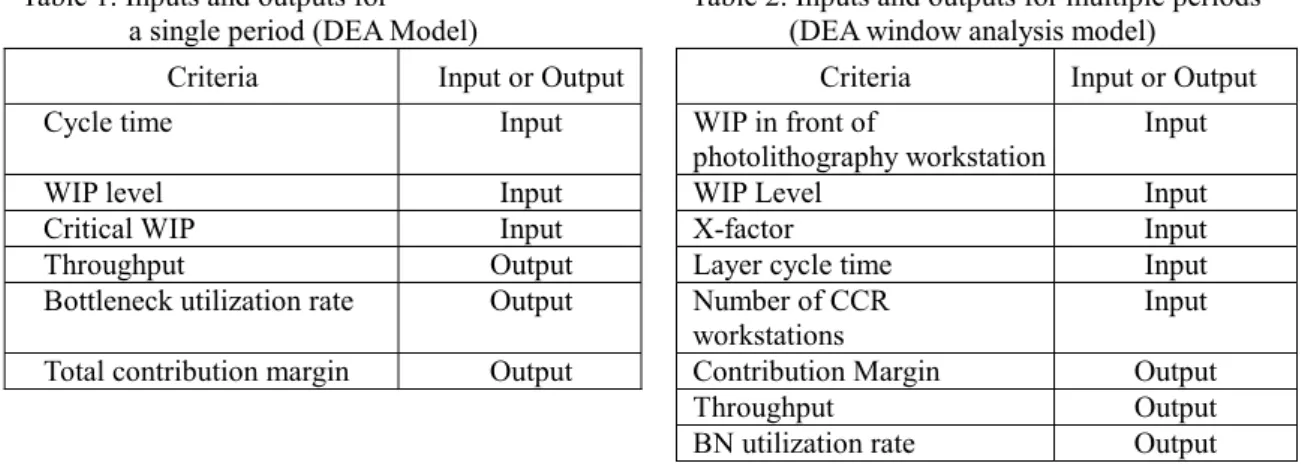
Criteria for product mix selection under a single period (DEA model) are (1), (2), (3), (4), (5) and (6), as shown in Table 1. Criteria for product family mix selection under multiple periods are (2), (4), (5), (6), (7), (8), (9) and (10), as shown in Table 2.
Table 1. Inputs and outputs for Table 2. Inputs and outputs for multiple periods a single period (DEA Model) (DEA window analysis model)
Criteria Input or Output Criteria Input or Output Cycle time Input WIP in front of
photolithography workstation Input WIP level Input WIP Level Input Critical WIP Input X-factor Input Throughput Output Layer cycle time Input Bottleneck utilization rate Output Number of CCR
workstations Input Total contribution margin Output Contribution Margin Output
Throughput Output
BN utilization rate Output
4.2 The selection of input and output factors
The selection of factors is essential. Factors should be selected properly to represent other correlated factors so as to reduce number of inputs and outputs for the DEA model. For evaluating the product (family) mixes in a semiconductor fab, data corresponding to these factors must meet the isotonicity
required by DEA in order to obtain acute evaluation results. Isotonicity means that when an input increases, an output should not decrease, and vice versa [18]. If one factor has a negative or very weak correlation with other inputs or outputs, in order to satisfy isotonicity, the factor needs to be deleted from the model. On the other hand, when two factors are perfectly positive correlated, that is, the correlation coefficient is 1, the changes of one factor can be reflected by the changes of the other factor completely. In this case, only one factor is needed to evaluate the system performance.
Based on the above requirements, the most suitable input and output factors can be selected by the following steps:
Step 1: Have an interview with the relevant personnel and managers in the industry and obtain input and output factors that are considered to be most important. These factors are the candidate factors. Step 2: Construct a virtual wafer fab by building a simulation model. Run this model under different
scenarios so as to collect the data of the candidate factors.
Step 3: Calculate the correlation coefficients among the candidate factors. If there is any factor that has a negative correlation with other factors, delete the factor.
Step 4: If there are any two or more factors that are perfectly positive correlated, select the factor that has higher correlations with the rest of the factors.
4.3 System environment under a single period (DEA model)
To investigate the possibility of obtaining a set of product mix that is most efficient for a given factory, actual data is taken from a wafer fabrication factory located on the Science-Based Industrial Park in Taiwan. Simulation result is applied to estimate the production performance. To simplify the complexity of the environment for our analysis, this paper is based on the following assumptions and limitations:
• The production system consists of two products, A and B. Both products are the logic product. There is only one priority level of products; that is, all products are normal. The process of each product type is different and unique.
• Product A requires 305 operations and passes through the bottleneck 17 times. That is, 18 layers are processed. Product B requires 345 operations and passes through the bottleneck 19 times (20 layers processed). There are both batch and serial types of machines, and a total of 83 workstations (W1 to W83) are in the production environment.
• Preventive maintenance is considered in estimating usable production capacity.
• WS46, a stepper in the photolithography area, is the bottleneck.
• Throughput target is given. For a period of 28 days, we set the throughput target to be 580, 600, 620, 640, 660 lots for various cases.
• Mix(1,9)-580 means that the product mix ratio for product A to product B is 1 to 9 and the throughput target is 580 lots.
• The releasing batch size for normal lots is six lots. Such a setting is for effective use of many workstations which have a maximum batch size (MBS) of six lots.
• Wafer lots are released under CONWIP, a constant work-in process (WIP) policy. Under each product mix with a fixed stated throughput target, the WIP level is first estimated through BBCT algorithm [14]and the value is the constant WIP input to the simulation model under this certain product mix. The throughput target can be achieved with less than 1% of variance by adopting the estimated WIP. For each product mix setting, the WIP level has to be estimated individually and is different under each case as a result.
• The dispatching rule is first-in, first-out (FIFO).
• Lots with different product types cannot be processed simultaneously.
• Product price is determined by the number of layers the product being processed. Because different products go through different processes, the charged price is set to be $40 per passing through the bottleneck for product A, and $50 for product B.
• Direct material cost, that is, cost of raw wafers, is assumed to be $100 per wafer. Indirect material cost, such as photo-resist, special gas, chemical and quartz, is varied according to the production level. The indirect material cost is set to be $7.5 per layer for product A, and $8 per layer for product B.
• A holding cost is considered for the WIP at an annual rate of 10%. Because CONWIP is adopted, WIP level is consistent throughout the period. Since material is the major variable cost of a product, the holding cost of material of the WIP will be calculated as: Total material cost of the WIP × holding rate for the period.
4.4 Results for single period (DEA model)
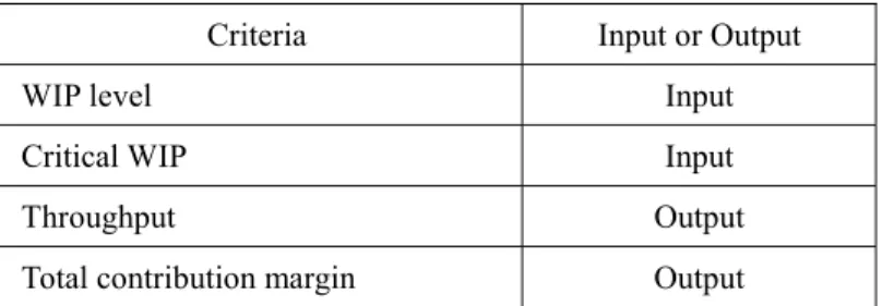
As discussed earlier, if one or more factors have a close relationship with another factor, it may be possible to exclude it from the DEA analysis. Therefore, correlation analysis is performed on all the inputs and outputs selected, and the results are shown in Table 3. WIP level and cycle time are highly positively correlated with a correlation coefficient of 0.96 due to the fact that as WIP level decreases and cycle time will also decrease under the same throughput (i.e. L=λW) [21]. Therefore, cycle time will not be considered in the analysis. The correlation coefficient between critical WIP and bottleneck utilization rate is 0.97, a significantly high value. Consequently, critical WIP is chosen to represent these two factors. The final inputs and outputs selected for the analysis will be as in Table 4.
Table 3. Correlation coefficient between the factors.
WIP level Critical WIP Throughput utilization rate Bottleneck Total Contribution Margin Cycle time 0.96 0.81 0.43 0.76 0.60 WIP level 0.86 0.67 0.87 0.72 Critical WIP 0.65 0.97 0.92
Throughput 0.81 0.77
Table 4. Input and output variables in DEA analysis. Criteria Input or Output WIP level Input Critical WIP Input
Throughput Output Total contribution margin Output
Based on the performance for each criterion, it is possible to rank the product mixes, as shown in Table 5. Different product mix performs differently in terms of individual performance criteria. The best and the worst product mix for each of the criteria are summarized below:
WIP level: best, Mix(9,1)-580; worst, Mix(1,9)-660. Critical WIP: best, Mix(9,1)-580; worst, Mix(1,9)-660.
Throughput: best, DMUs with throughput of 660; worst, DMUs with throughput of 580. Total contribution margin: best, Mix(2,8)-660; worst, Mix(9,1)-580.
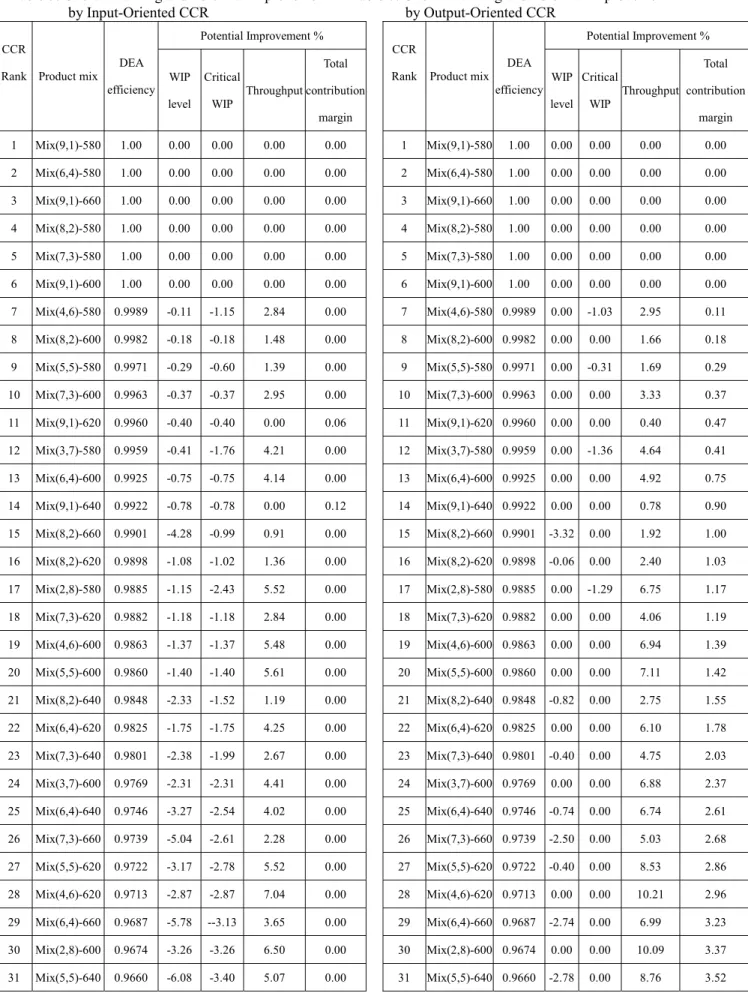
For DEA model, a mathematical programming software package, CPLEX, is used for the computations. Input/output-oriented CCR model is first run under the assumption of constant returns to scale, and input/output-oriented BCC models is run next under the assumption of variable returns to scale. The technical efficiency and scale efficiency of each DMU will also be calculated, and the analysis is made. For the CCR model, two input variables (WIP level, Critical WIP) and two output variables (throughput and total contribution margin) are considered, and the results are shown in Table 5 and 6. As indicated earlier, under the assumption of constant returns to scale, the technical efficiency results obtained from the input minimization approach and output maximization approach are the same. That is, the outcomes under input-oriented CCR (CCRp-I) and output-oriented CCR (CCRp-O) are the same. A total of 6 DMUs are found to be efficient. It should be noted that the DEA efficiencies do not represent absolute ratings for the product mix. They only represent relative ratings among the DMUs selected. For example, we can only say that Mix(7,3)-660 is less efficient than Mix(6,4)-580 under the criteria considered.
To illustrate this, Mix(1,9)-580 has a reference set of Mix(7,3)-580 and Mix(8,2)-580. That is, by compared with Mix(7,3)-580 and Mix(8,2)-580, two efficient DMUs, Mix(1,9)-580 is relatively inefficient. While the three DMUs has the same level of throughput-(580), an output, Mix(7,3)-580 and Mix(8,2)-580 both have fewer inputs (WIP level and critical WIP) than those of Mix(1,9)-580. Although the other output (total contribution margin) for Mix(1,9)-580 is higher than those of the two efficient DMUs, the performance of this output is not good enough to make Mix(1,9)-580 to be efficient. Also listed in Table 6 are the values of the slack variables, si- and sr+ from equation (1), corresponding, respectively, to the two
inputs (i=1, WIP; i=2, critical WIP) and two outputs (r=1, throughput; r=2. Total contribution margin). A study of slack values can provide us with projections for where the inputs and outputs must be for that DMU to be efficient. This information allows us to set the target, which could guide inefficient DMUs to improve performance. For efficient DMUs, the actual and target inputs (outputs) are all equal, and the potential improvements as a result are zero’s, as shown in Table 5. For inefficient DMUs we can know how they can be improved to be efficient. For example, under input-oriented CCR, Mix(1,9)-640 has an efficient score of 0.9208. From the potential improvement in Table 5, we can see that based on input the DMU can
decrease the cycle time by up to 16.46% or critical WIP by up to 7.92% to be more efficient. Based on output, it can increase the total contribution margin by 8.92% to be efficient.
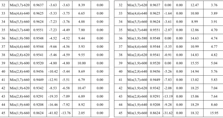
As a general rule, if on the average the excess of a certain input/output is very low, that variable is considered critical in determining the efficiency value of DMUs. For example, total contribution margin is a critical variable since the potential improvement values for the total contribution margin are mostly zero’s for DMUs. This implies that the total contribution margin performs considerably well in most DMUs than other input/output parameters. Therefore, for efficient purpose, the decision maker should focus their effort on the improvement for the other factors. From the output maximization perspective, the potential improvements for the inputs/output variables are shown in Table 6. Critical WIP, with mostly zero excess values, is also a critical variable in determining the efficiency of DMUs, which has mostly zero potential improvement for DMUs. We can also compromise the input-oriented and output-oriented models by averaging the projected values. For example, the potential improvements for Mix(1,9)-660 will be a decrease of the WIP level by 36.32%, a decrease of the critical WIP by 6.88%, an increase of the throughput by 10.19%, and an increase of the total contribution margin by 7.98%.
It is worthwhile to note that if we decrease the WIP level, other factors such as the critical WIP, the throughput, and the total contribution margin, could change in the production, but the impact may be consistent or tradeoffs. We observe that when the WIP level decreases, the critical WIP needs to be reduced, which may not be beneficial to the throughput. Therefore, to increase the throughput the WIP level should be increased. Keeping a queue of lots at each process insures that the equipment be in busy status and the utilization rate becomes high. However, as the WIP level continues to be increasing, the factory will become congested with inventory and throughput reflects a polynomial growth and may even decrease at last. Therefore, a WIP level that is too low or too high is neither desirable. In conclusion, given a set of criteria, DEA can provide goals for the DMU be efficient. However, the choice of input and output parameter will affect the outcome of the efficiency, and the inter-relationship among the criteria may influence the actual improvement of the system.
Based on the assumption of variable returns to scale, both the input-oriented BCC (BCCp-I) and the output-oriented BCC (BCCp-O) models are applied (two inputs and two outputs). The results are shown in Table 7 and 8. Even though the 31 DMUs that are efficient under the input-oriented BCC are also efficient under the output-oriented BCC, the ranking and efficiency score of the rest of DMUs are not the same under the two approaches. The potential improvements under the two approaches are also different. For the input-oriented BCC, the improvement of inputs is stressed. That is, reducing the amount of input values will lead a DMU to be more efficient. For output-oriented BCC, the results are opposite. That is, to increase the amount of output values should be the major effort.
To summarize the result, six DMUs are found to be efficient under CCR, input-oriented BCC, output-oriented BCC analysis: Mix(6,4)-580, Mix(7,3)-580, Mix(8,2)-580, Mix(9,1)-580, Mix(9,1)-600, and Mix(9,1)-660. Therefore, if we accept orders based on the above six product mixes and set the throughput level accordingly, we can achieve an efficient production performance. On the other hand, if the throughput level is predetermined, we can accept orders based on the product mix that has the highest efficiency score. For example, if constant returns to scale is assumed and the throughput level is set to be 620 lots, Mix(9,1) will be selected since it has the highest score of .9960 compared to the other mixes under the throughput level of 620 lots.
Table 5. Overall Ranking and Potential Improvement Table 6. Overall Ranking and Potential Improvement by Input-Oriented CCR by Output-Oriented CCR
Potential Improvement % Potential Improvement %
CCR
Rank Product mix
DEA efficiency WIP level Critical WIP Throughput Total contribution margin CCR
Rank Product mix
DEA efficiency WIP level Critical WIP Throughput Total contribution margin 1 Mix(9,1)-580 1.00 0.00 0.00 0.00 0.00 1 Mix(9,1)-580 1.00 0.00 0.00 0.00 0.00 2 Mix(6,4)-580 1.00 0.00 0.00 0.00 0.00 2 Mix(6,4)-580 1.00 0.00 0.00 0.00 0.00 3 Mix(9,1)-660 1.00 0.00 0.00 0.00 0.00 3 Mix(9,1)-660 1.00 0.00 0.00 0.00 0.00 4 Mix(8,2)-580 1.00 0.00 0.00 0.00 0.00 4 Mix(8,2)-580 1.00 0.00 0.00 0.00 0.00 5 Mix(7,3)-580 1.00 0.00 0.00 0.00 0.00 5 Mix(7,3)-580 1.00 0.00 0.00 0.00 0.00 6 Mix(9,1)-600 1.00 0.00 0.00 0.00 0.00 6 Mix(9,1)-600 1.00 0.00 0.00 0.00 0.00 7 Mix(4,6)-580 0.9989 -0.11 -1.15 2.84 0.00 7 Mix(4,6)-580 0.9989 0.00 -1.03 2.95 0.11 8 Mix(8,2)-600 0.9982 -0.18 -0.18 1.48 0.00 8 Mix(8,2)-600 0.9982 0.00 0.00 1.66 0.18 9 Mix(5,5)-580 0.9971 -0.29 -0.60 1.39 0.00 9 Mix(5,5)-580 0.9971 0.00 -0.31 1.69 0.29 10 Mix(7,3)-600 0.9963 -0.37 -0.37 2.95 0.00 10 Mix(7,3)-600 0.9963 0.00 0.00 3.33 0.37 11 Mix(9,1)-620 0.9960 -0.40 -0.40 0.00 0.06 11 Mix(9,1)-620 0.9960 0.00 0.00 0.40 0.47 12 Mix(3,7)-580 0.9959 -0.41 -1.76 4.21 0.00 12 Mix(3,7)-580 0.9959 0.00 -1.36 4.64 0.41 13 Mix(6,4)-600 0.9925 -0.75 -0.75 4.14 0.00 13 Mix(6,4)-600 0.9925 0.00 0.00 4.92 0.75 14 Mix(9,1)-640 0.9922 -0.78 -0.78 0.00 0.12 14 Mix(9,1)-640 0.9922 0.00 0.00 0.78 0.90 15 Mix(8,2)-660 0.9901 -4.28 -0.99 0.91 0.00 15 Mix(8,2)-660 0.9901 -3.32 0.00 1.92 1.00 16 Mix(8,2)-620 0.9898 -1.08 -1.02 1.36 0.00 16 Mix(8,2)-620 0.9898 -0.06 0.00 2.40 1.03 17 Mix(2,8)-580 0.9885 -1.15 -2.43 5.52 0.00 17 Mix(2,8)-580 0.9885 0.00 -1.29 6.75 1.17 18 Mix(7,3)-620 0.9882 -1.18 -1.18 2.84 0.00 18 Mix(7,3)-620 0.9882 0.00 0.00 4.06 1.19 19 Mix(4,6)-600 0.9863 -1.37 -1.37 5.48 0.00 19 Mix(4,6)-600 0.9863 0.00 0.00 6.94 1.39 20 Mix(5,5)-600 0.9860 -1.40 -1.40 5.61 0.00 20 Mix(5,5)-600 0.9860 0.00 0.00 7.11 1.42 21 Mix(8,2)-640 0.9848 -2.33 -1.52 1.19 0.00 21 Mix(8,2)-640 0.9848 -0.82 0.00 2.75 1.55 22 Mix(6,4)-620 0.9825 -1.75 -1.75 4.25 0.00 22 Mix(6,4)-620 0.9825 0.00 0.00 6.10 1.78 23 Mix(7,3)-640 0.9801 -2.38 -1.99 2.67 0.00 23 Mix(7,3)-640 0.9801 -0.40 0.00 4.75 2.03 24 Mix(3,7)-600 0.9769 -2.31 -2.31 4.41 0.00 24 Mix(3,7)-600 0.9769 0.00 0.00 6.88 2.37 25 Mix(6,4)-640 0.9746 -3.27 -2.54 4.02 0.00 25 Mix(6,4)-640 0.9746 -0.74 0.00 6.74 2.61 26 Mix(7,3)-660 0.9739 -5.04 -2.61 2.28 0.00 26 Mix(7,3)-660 0.9739 -2.50 0.00 5.03 2.68 27 Mix(5,5)-620 0.9722 -3.17 -2.78 5.52 0.00 27 Mix(5,5)-620 0.9722 -0.40 0.00 8.53 2.86 28 Mix(4,6)-620 0.9713 -2.87 -2.87 7.04 0.00 28 Mix(4,6)-620 0.9713 0.00 0.00 10.21 2.96 29 Mix(6,4)-660 0.9687 -5.78 --3.13 3.65 0.00 29 Mix(6,4)-660 0.9687 -2.74 0.00 6.99 3.23 30 Mix(2,8)-600 0.9674 -3.26 -3.26 6.50 0.00 30 Mix(2,8)-600 0.9674 0.00 0.00 10.09 3.37 31 Mix(5,5)-640 0.9660 -6.08 -3.40 5.07 0.00 31 Mix(5,5)-640 0.9660 -2.78 0.00 8.76 3.52
32 Mix(3,7)-620 0.9637 -3.63 -3.63 8.39 0.00 32 Mix(3,7)-620 0.9637 0.00 0.00 12.47 3.76 33 Mix(4,6)-640 0.9625 -5.33 -3.75 6.65 0.00 33 Mix(4,6)-640 0.9625 -1.64 0.00 10.80 3.89 34 Mix(5,5)-660 0.9624 -7.23 -3.76 4.88 0.00 34 Mix(5,5)-660 0.9624 -3.61 0.00 8.99 3.91 35 Mix(3,7)-640 0.9551 -7.23 -4.49 7.80 0.00 35 Mix(3,7)-640 0.9551 -2.87 0.00 12.86 4.70 36 Mix(1,9)-580 0.9548 -4.52 -4.52 9.44 0.00 36 Mix(1,9)-580 0.9548 0.00 0.00 14.63 4.74 37 Mix(4,6)-660 0.9544 -9.66 -4.56 5.93 0.00 37 Mix(4,6)-660 0.9544 -5.35 0.00 10.99 4.77 38 Mix(2,8)-620 0.9541 -5.46 -4.59 9.55 0.00 38 Mix(2,8)-620 0.9541 -0.91 0.00 14.83 4.82 39 Mix(1,9)-600 0.9520 -4.80 -4.80 10.00 0.00 39 Mix(1,9)-600 0.9520 0.00 0.00 15.55 5.04 40 Mix(2,8)-640 0.9456 -10.42 -5.44 8.69 0.00 40 Mix(2,8)-640 0.9456 -5.26 0.00 14.94 5.76 41 Mix(3,7)-660 0.9449 -12.91 -5.51 6.79 0.00 41 Mix(3,7)-660 0.9449 -7.83 0.00 13.02 5.83 42 Mix(1,9)-620 0.9342 -8.53 -6.58 10.47 0.00 42 Mix(1,9)-620 0.9342 -2.08 0.00 18.25 7.04 43 Mix(2,8)-660 0.9291 -19.35 -7.09 6.89 0.00 43 Mix(2,8)-660 0.9291 -13.19 0.00 15.06 7.64 44 Mix(1,9)-640 0.9208 -16.46 -7.92 8.92 0.00 44 Mix(1,9)-640 0.9208 -9.28 0.00 18.29 8.60 45 Mix(1,9)-660 0.8624 -41.02 -13.76 2.05 0.00 45 Mix(1,9)-660 0.8624 -31.62 0.00 18.32 15.95
Table 7. Overall Ranking and Potential Improvement Table 8. Overall Ranking and Potential Improvement by Input-Oriented BCC by Output-Oriented BCC
Potential Improvement % Potential Improvement %
CCR
Rank Product mix DEA
efficiency WIP level Critical WIP Throughput Total contribution margin CCR
Rank Product mix DEA
efficiency WIP level Critical WIP Throughput Total contribution margin 1 Mix(3,7)-660 1.00 0.00 0.00 0.00 0.00 1 Mix(9,1)-580 1.00 0.00 0.00 0.00 0.00 2 Mix(2,8)-660 1.00 0.00 0.00 0.00 0.00 2 Mix(9,1)-660 1.00 0.00 0.00 0.00 0.00 3 Mix(5,5)-660 1.00 0.00 0.00 0.00 0.00 3 Mix(4,6)-580 1.00 0.00 0.00 0.00 0.00 4 Mix(4,6)-660 1.00 0.00 0.00 0.00 0.00 4 Mix(3,7)-580 1.00 0.00 0.00 0.00 0.00 5 Mix(9,1)-580 1.00 0.00 0.00 0.00 0.00 5 Mix(8,2)-580 1.00 0.00 0.00 0.00 0.00 6 Mix(4,6)-640 1.00 0.00 0.00 0.00 0.00 6 Mix(7,3)-580 1.00 0.00 0.00 0.00 0.00 7 Mix(3,7)-620 1.00 0.00 0.00 0.00 0.00 7 Mix(8,2)-600 1.00 0.00 0.00 0.00 0.00 8 Mix(4,6)-580 1.00 0.00 0.00 0.00 0.00 8 Mix(7,3)-600 1.00 0.00 0.00 0.00 0.00 9 Mix(3,7)-580 1.00 0.00 0.00 0.00 0.00 9 Mix(2,8)-660 1.00 0.00 0.00 0.00 0.00 10 Mix(9,1)-640 1.00 0.00 0.00 0.00 0.00 10 Mix(6,4)-580 1.00 0.00 0.00 0.00 0.00 11 Mix(9,1)-660 1.00 0.00 0.00 0.00 0.00 11 Mix(3,7)-660 1.00 0.00 0.00 0.00 0.00 12 Mix(2,8)-600 1.00 0.00 0.00 0.00 0.00 12 Mix(9,1)-640 1.00 0.00 0.00 0.00 0.00 13 Mix(7,3)-600 1.00 0.00 0.00 0.00 0.00 13 Mix(8,2)-640 1.00 0.00 0.00 0.00 0.00 14 Mix(8,2)-640 1.00 0.00 0.00 0.00 0.00 14 Mix(9,1)-600 1.00 0.00 0.00 0.00 0.00 15 Mix(2,8)-580 1.00 0.00 0.00 0.00 0.00 15 Mix(2,8)-580 1.00 0.00 0.00 0.00 0.00 16 Mix(8,2)-660 1.00 0.00 0.00 0.00 0.00 16 Mix(3,7)-600 1.00 0.00 0.00 0.00 0.00 17 Mix(7,3)-660 1.00 0.00 0.00 0.00 0.00 17 Mix(4,6)-660 1.00 0.00 0.00 0.00 0.00
18 Mix(4,6)-600 1.00 0.00 0.00 0.00 0.00 18 Mix(9,1)-620 1.00 0.00 0.00 0.00 0.00 19 Mix(4,6)-620 1.00 0.00 0.00 0.00 0.00 19 Mix(6,4)-600 1.00 0.00 0.00 0.00 0.00 20 Mix(3,7)-600 1.00 0.00 0.00 0.00 0.00 20 Mix(7,3)-620 1.00 0.00 0.00 0.00 0.00 21 Mix(6,4)-660 1.00 0.00 0.00 0.00 0.00 21 Mix(4,6)-600 1.00 0.00 0.00 0.00 0.00 22 Mix(7,3)-640 1.00 0.00 0.00 0.00 0.00 22 Mix(2,8)-600 1.00 0.00 0.00 0.00 0.00 23 Mix(8,2)-580 1.00 0.00 0.00 0.00 0.00 23 Mix(7,3)-640 1.00 0.00 0.00 0.00 0.00 24 Mix(7,3)-580 1.00 0.00 0.00 0.00 0.00 24 Mix(8,2)-660 1.00 0.00 0.00 0.00 0.00 25 Mix(6,4)-580 1.00 0.00 0.00 0.00 0.00 25 Mix(3,7)-620 1.00 0.00 0.00 0.00 0.00 26 Mix(6,4)-640 1.00 0.00 0.00 0.00 0.00 26 Mix(7,3)-660 1.00 0.00 0.00 0.00 0.00 27 Mix(9,1)-620 1.00 0.00 0.00 0.00 0.00 27 Mix(4,6)-640 1.00 0.00 0.00 0.00 0.00 28 Mix(6,4)-600 1.00 0.00 0.00 0.00 0.00 28 Mix(6,4)-660 1.00 0.00 0.00 0.00 0.00 29 Mix(7,3)-620 1.00 0.00 0.00 0.00 0.00 29 Mix(4,6)-620 1.00 0.00 0.00 0.00 0.00 30 Mix(8,2)-600 1.00 0.00 0.00 0.00 0.00 30 Mix(5,5)-660 1.00 0.00 0.00 0.00 0.00 31 Mix(9,1)-600 1.00 0.00 0.00 0.00 0.00 31 Mix(6,4)-640 1.00 0.00 0.00 0.00 0.00 32 Mix(8,2)-620 0.9989 -0.11 -0.11 0.00 0.00 32 Mix(1,9)-660 1.00 -37.41 -11.84 0.00 0.00 33 Mix(6,4)-620 0.9989 -0.11 -0.11 0.00 0.00 33 Mix(6,4)-620 0.9992 0.00 0.00 0.08 0.08 34 Mix(5,5)-580 0.9983 -0.17 -0.17 0.23 0.00 34 Mix(8,2)-620 0.9991 0.00 0.00 0.09 0.09 35 Mix(5,5)-600 0.9974 -0.26 -0.26 0.80 0.00 35 Mix(5,5)-580 0.9986 0.00 0.00 0.29 0.15 36 Mix(3,7)-640 0.9953 -0.47 -0.76 2.38 0.00 36 Mix(3,7)-640 0.9981 0.00 -0.56 2.81 0.19 37 Mix(2,8)-620 0.9921 -0.79 -0.86 2.18 0.00 37 Mix(5,5)-600 0.998 0.00 0.00 0.92 0.21 38 Mix(1,9)-600 0.9910 -0.90 -1.62 2.05 0.00 38 Mix(2,8)-620 0.9966 0.00 -0.54 2.90 0.34 39 Mix(5,5)-620 0.9900 -1.00 -1.00 1.55 0.00 39 Mix(1,9)-600 0.9953 0.00 -1.51 2.96 0.47 40 Mix(2,8)-640 0.9865 -2.17 -1.35 3.12 0.00 40 Mix(2,8)-640 0.9943 0.00 -0.29 3.12 0.57 41 Mix(5,5)-640 0.9855 -1.45 -1.45 2.53 0.00 41 Mix(5,5)-620 0.9932 0.00 0.00 2.93 0.68 42 Mix(1,9)-620 0.9711 -2.89 -2.94 4.00 0.00 42 Mix(5,5)-640 0.9914 0.00 0.00 2.87 0.87 43 Mix(1,9)-580 0.9693 -3.07 -3.07 3.62 0.00 43 Mix(1,9)-640 0.9887 0.00 -0.78 3.12 1.15 44 Mix(1,9)-640 0.9624 -8.25 3.76 3.12 0.00 44 Mix(1,9)-620 0.9885 0.00 -1.72 6.45 1.16 45 Mix(1,9)-660 0.8785 -37.81 -12.15 0.00 0.00 45 Mix(1,9)-580 0.9817 0.00 0.00 4.77 1.87
4.5 System environment under multiple periods (DEA window analysis)
In order to obtain a set of product family mixes that is efficient for the factory to manufacture, actual data is collected from a wafer fabrication factory located on the Science-Based Industrial Park in Taiwan. A simulation model is developed by EM-Plant [32] to generate relevant production performance factors. Simulation results are then applied in the DEA window analysis to convert the performance results under each product family mix over time into an overall efficiency score. To simplify the complexity of the environment, the simulation model built in this paper is based on the following assumptions and limitations:
• There are two different product family types. Product family A consists of a variety of logic products, and product family B consists of memory products. The process of each product family is different and unique.
• Products belonging to family A require 305 operations and pass through the photolithography operation 17 times. Products in family B require 330 operations and pass through the photolithography operation 20 times.
• There are 83 different types of workstations, with thirteen 6-lot workstations, three 4-lot workstations, and nineteen 2-lot workstations. Each workstation consists of a given number of identical machines operated in parallel.
• The lot priority is classed into hot, rush and normal in descending order. The ratio of priorities for each product family is set to be 1, 2, and 7 for hot, rush and normal classes, respectively.
• Wafer lot(s) can be released to shop floor only when the same quantity of wafers are finished and transferred out. The releasing batch size for both normal and rush lots is six lots. Batch machines adopt full batch size policy. Once batch forming is completed, processing sequence is based on the priority class and FIFO rule.
• The hot orders are not limited by batching policy, and they can be released into shop floor and be loaded onto any batch machine with only a single lot.
• Lots with different product types and classes cannot be processed simultaneously.
• The charged price for product with normal priority is set to be $40 per passing through the photolithography operation for product family A, and $50 for product family B. Because the waiting time for higher priority orders is shorter than that for normal orders, the charged prices for hot and rush priority products are set to be 150% and 50% mark-up of the price for normal product, respectively.
• Direct material cost is set to be $100 per wafer. Indirect material cost, such as photo-resist, special gas, chemical and quartz, is varied according to the production family. The indirect material cost is assumed to be $7.5 per layer for product family A, and $8 per layer for product family B.
• The observation period is seven years, and the throughput target is set to be 420 lots, 620 lots, 640 lots, 464 lots, 343 lots, 387 lots and 526 lots per month for year 1 to year 7 respectively. The window length is fixed to be three years (K=3).
• Product family mixes are set between (2:8) to (8:2). Mix (2:8) means that the product family mix ratio for product family A to product family B is 2 to 8.
The simulation model is run 15 times to generate statistical results under each product family mix and each throughput target.
4.6 Results for multiple periods (DEA window analysis)
given throughput target and product family mix. Table 9 shows the monthly throughput targets and average monthly throughput outcomes under different product family mixes in each year. Note that the predetermined throughput targets and the outcomes from the simulation model may not be the same. In order to maintain a fair evaluation, only the simulation results with throughput deviation of less than five batches from the predetermined throughput target are collected. A partial data of the collected candidate factors under different environments is shown in Table 10.
Based on the procedures stated in Section 4.2, a correlation analysis of the factors is done by STATISTICA 6.0 [28] to check if there is any factor that has a negative correlation coefficient or perfect positive correlation with other factors. The correlation coefficient of the input and output factors are shown in Table 11. The correlation coefficient between throughput and bottleneck utilization rate is exactly one. Since the correlation coefficients of bottleneck utilization rate with other factors are higher than the coefficients of throughput with other factors, throughput is deleted from the list. The input and output factors selected for evaluation of the wafer fab are listed in Table 12.
With the simulation results of the selected factors, DEA window analysis can be done by Excel Solver via Visual Basic application [15]. In this paper, we assume constant returns to scale; that is, as all inputs double, all outputs will double. The overall efficiency for each DMU is calculated by using CCRd-I model, and the DEA window analysis is applied. These results are shown in Table 13.
Table 9. Throughput targets and average throughput outcomes Product family mix Monthly throughput target (lot) 420 620 640 464 343 387 526 Mix (2,8) 423 625 637 468 345 388 525 Mix (3,7) 420 615 645 469 338 392 529 Mix (4,6) 424 620 645 466 343 392 530 Mix (5,5) 420 618 642 465 348 392 525 Mix (6,4) 423 624 645 465 347 382 523 Mix (7,3) 419 624 641 462 341 387 529 Mix (8,2) Real average throughput target (lot) 425 617 635 459 348 390 524
Table 10. Simulation results for candidate factors under Mix (2,8) Year (throughput target) WIP in front of photolithography workstation (lot) Throughput (lot) BN utilization rate Number of CCR workstations WIP level (lot) Layer cycle time (second) X-factor Contribution margin ($) Year 1 (420 lots) 8 423 0.638 0 187 53192 1.41 106,149,525 Year 2 21 625 0.927 8 306 60043 1.59 156,543,300
(620 lots) Year 3 (640 lots) 26 637 0.963 10 319 61354 1.63 161,580,325 Year 4 (464 lots) 10 468 0.700 0 206 53797 1.43 117,118,625 Year 5 (343 lots) 6 345 0.517 0 151 52422 1.39 86,856,600 Year 6 (387 lots) 8 388 0.577 0 169 52657 1.40 97,129,975 Year 7 (526 lots) 11 525 0.779 2 236 55219 1.46 131,401,475
Table 11. Correlation analysis of candidate factors Throughput (lot) BN utilization rate Number of CCR workstations WIP Level (lot) Layer cycle time (second) X-factor Contribution margin ($) WIP in front of photolithography workstation (lot) 0.94 0.94 0.91 0.97 0.96 0.92 0.85 Throughput (lot) 1.00 1.00 0.82 0.99 0.89 0.85 0.90 BN utilization rate 1.00 0.84 0.99 0.89 0.86 0.91 Number of CCR workstations 1.00 0.88 0.87 0.85 0.82 WIP Level(lot) 1.00 0.93 0.91 0.93 Layer cycle time
(second) 1.00 0.97 0.83 X-factor 1.00 0.88
Table 12. Input and output factors for evaluation
Factor Input or Output Layer cycle time Input WIP in front of photolithography workstation Input WIP Level Input BN utilization rate Output Contribution Margin Output Number of CCR workstations Input
X-factor Input
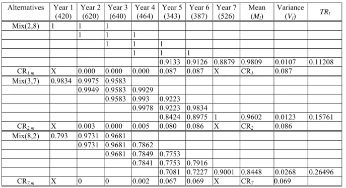
Table 13. Window analysis of alternatives Alternatives Year 1
(420) Year 2 (620) Year 3(640) Year 4(464) Year 5(343) Year 6(387) Year 7(526) Mean (Ml)
Variance (Vl) TRl Mix(2,8) 1 1 1 1 1 1 1 1 1 1 1 1 1 1 0.991 0.9994 0.0006 0.0086 CR1,m X 0 0 0 0 0 X CR1 0 Mix(3,7) 1 1 0.988 1 0.980 1 1 1 0.995 1 0.995 1
0.995 1 1 0.9970 0.0015 0.0199 CR2,m X 0 0.02 0 0 0 X CR2 0.0199 Mix(4,6) 0.998 1 0.948 1 0.945 0.990 0.981 0.990 0.973 0.990 0.973 0.999 0.973 1 1 0.9839 0.0049 0.0549 CR3,m X 0 0.036 0 0 0.001 X CR3 0.0358 Mix(5,5) 0.960 0.985 0.950 0.981 0.950 0.982 1 0.981 0.975 0.981 0.975 0.969 0.978 0.996 0.976 0.9759 0.0038 0.0503 CR4,m X 0.004 0.050 0 0.004 0.027 X CR4 0.0503 Mix(6,4) 1 1 0.933 1 0.931 0.978 0.984 0.976 1 0.976 1 0.980 1 0.987 0.997 0.9828 0.0061 0.0694 CR5,m X 0 0.053 0.001 0 0.007 X CR5 0.0530 Mix(7,3) 1 1 0.967 1 0.967 1 1 1 1 1 0.990 0.945 0.990 0.955 1 0.9877 0.0051 0.0545 CR6,m X 0 0.033 0 0.010 0.010 X CR6 0.0327 Mix(8,2) 1 0.973 0.966 0.973 0.966 1 1 1 1 1 1 1 1 1 1 0.9919 0.0038 0.0340 CR7,m X 0 0.034 0 0 0 X CR7 0.0340 Observing the average efficiency values, Mix (2,8) is the highest with a mean of 0.9994. On top of that, this product family has the lowest variance of 0.0006. In a highly variant demand changing environment, Mix (2,8) has a quite stabilized performance over the years.
The second and third best product family mixes are Mix (3,7) and Mix (8,2). Both mixes maintain relatively high efficiency over the periods, and their variances are not too big either; therefore, the overall performances of the system under these two mixes are quite stabilized too. Regarding the CR value, the best mix is Mix (2,8), and the second best is Mix (3,7). Mix (2,8) also has the best TR value of 0.0086, followed by Mix (3,7) and Mix (8,2).
With the overall evaluation, the best mix is Mix (2,8), and Mix (3,7) and Mix (8,2) perform quite well too. In fact, the performances under Mix (2,8), Mix (3,7) and Mix (8,2) are not significantly different. Therefore, these three mixes are further evaluated. Since financial success is the ultimate goal for an enterprise, only the financial factors, contribution margin, X-factor and WIP level, are considered here, and the results are shown in Table 14.
Under the window analysis of the three product family mixes by focused on financial aspect, Mix (2,8) and Mix (3,7) perform well than Mix (8,2) in efficiency mean, variance and total range. In addition, Mix (2,8) performs better than both Mix (3,7) and Mix (8,2) in all aspects. This implies that if the fab is able to maintain such a product family mix in a long term, it can be competitive and make a very reasonable
profit. In the case that the fab need be flexible in order acceptable, then it should concentrate its product mix in a range from Mix (2,8) to Mix(3,7), and preferably Mix (2,8).
Table 14. Window analysis of the top three alternatives by CCRd-I and CCRd-O Alternatives Year 1
(420) Year 2 (620) Year 3(640) Year 4(464) Year 5(343) Year 6(387) Year 7(526) Mean (Ml)
Variance (Vl) TRl Mix(2,8) 1 1 1 1 1 1 1 1 1 1 1 1 0.9133 0.9126 0.8879 0.9809 0.0107 0.11208 CR1,m X 0.000 0.000 0.000 0.087 0.087 X CR1 0.087 Mix(3,7) 0.9834 0.9975 0.9583 0.9949 0.9583 0.9929 0.9583 0.993 0.9223 0.9978 0.9223 0.9834 0.8424 0.8975 1 0.9602 0.0123 0.15761 CR2,m X 0.003 0.000 0.005 0.080 0.086 X CR2 0.086 Mix(8,2) 0.793 0.9731 0.9681 0.9731 0.9681 0.7862 0.9681 0.7849 0.7753 0.7841 0.7753 0.7916 0.7081 0.7227 0.9001 0.8448 0.0268 0.26496 CR7,m X 0 0 0.002 0.067 0.069 X CR7 0.069 5. Conclusion
This project applied the DEA method and the DEA window analysis to evaluate the production performance with different product (family) mixes in a semiconductor fabricator.
1. The research results of this project as below:
Without assigning weights to any performance measure, we used DEA to evaluate the efficiency of different product mixes, and obtained optimal product mix that is most efficient for production. The results provide guidance to the fabricator regarding accepting orders, which not only maximizes the production efficiency and hence the profit, but also considers several other important input and output factors that maintain production smoothing.
For the single period problem, a virtual wafer fab is first constructed, production with various product mix is simulated, and simulation results of critical performance factors are collected. The DEA method is then applied to analyze the results with different product mixes. Under the assumption of constant returns to scale, we used the CCR model to find the most efficient product mix. Under the assumption of variable returns to scale, input-oriented BCC and output-oriented BCC are used. In order to examine whether the DMUs are under an efficient production scale, input-oriented scale efficiency and output-oriented scale efficiency analysis are performed. The comprehensive analysis resulted in a set of efficient product mixes.
A DEA window analysis model is established to evaluate product family mixes in a wafer fab for the practice. A virtual wafer fab is constructed, production with various product family mixes over several periods of time is simulated, and simulation results of critical performance factors are collected. The DEA window analysis is then applied to analyze the results of different product family mixes over time, and the
mixes with higher performance are selected. For the selected mixes, another DEA window analysis is run based on a reduced number of factors that are the highest concern of the management, and the most recommended product family mix can be generated. The results not only try to maximize the production efficiency and hence the profit, but also considers several other important input and output factors that maintain production smoothing. By adopting the proposed mechanism, a semiconductor fabricator can have a guidance regarding strategies for order management and aggregate planning to improve manufacturing efficiency and to be competitive.
2. The research of this project has submit to: The relative result of the first year:
1. Shu-Hsing Chung, Chun-Mei Lai, Amy Hsin-I Lee and Hsin-E Lee, July 25-29, 2004, “The construction of production planning mechanism for wafer fabrication under demand variate environment,” 2004 Summer Computer Simulation Conference, San Jose, CA.
The relative result of the second year:
2. Shu-Hsing Chung and Chun-Mei Lai, “Job releasing and throughput planning for wafer fabrication under demand fluctuating make-to-stock environment”, International Journal of Advanced Manufacturing Technology, accepted.
3. Chung, S. H., W. L. Pearn and Amy H. I. Lee, 2004, “Measuring Production Performance with Different Product Mixes in Semiconductor Fabricator Using Data Envelopment Analysis (DEA),” International Journal of Industrial Engineering, Accepted. (SCI)
The relative result of the third year:
4. Shu-Hsing Chung, W. L. Pearn and Amy H. I. Lee, “Measuring production performance with different product mixes in semiconductor fabricator using data envelopment analysis (DEA),” International Journal of Industrial Engineering, accepted. (SCI)
5. Shu-Hsing Chung, Amy H. I. Lee, Chih-Wei Lai and Wen-Xuan Tseng, “A DEA window analysis on the product family mix selection for a Semiconductor Fabricator,” Omega- International Journal of Management Science, submitted.
6. Shu-Hsing Chung, Wen-Lea Pearn, Amy Hsin-I Lee and He-Yau Kang, Oct. 24, 2002, “Measuring efficiency of product mixes under a semiconductor fabricator using data envelopment analysis (DEA),” 2002 Semiconductor Manufacturing Technology Workshop, Hsinchu, Taiwan.
7. Shu-Hsing Chung, Wen-Lea Pearn, Amy Hsin-I Lee and He-Yau Kang, Dec. 6, 2003, “Product mix selection for two-level priority orders under a semiconductor fabricator by using data envelopment analysis (DEA),” Chinese Institute of Industrial Engineers Conference, Changhua, Taiwan.
8. Shu-Hsing Chung, Amy Hsin-I Lee, Chih-Wei Lai and Wen-Xuan Tseng, Dec. 18, 2004, “Product family mix selection for a semiconductor fabricator by using DEA window analysis,” Chinese Institute of Industrial Engineers Conference, Tainan, Taiwan.
6. REFERENCES
[1] Asmild M, Paradi JC, Aggarwall V, Schaffnit C. Combining DEA window analysis with the Malmquist index approach in a study of the Canadian banking industry. Journal of Productivity Analysis 2004; 21: 67-89.