國 立 交 通 大 學
電信工程研究所
碩 士 論 文
時槽式光叢集交換環中波長分配
與訊務控制
Wavelength Assignment and Traffic Control
(WATC) in Slotted OBS Rings
研 究 生:謝耀庭
指導教授:張仲儒 博士
時槽式光叢集交換環中波長分配與訊務控制
Wavelength Assignment and Traffic Control (WATC) in Slotted
OBS Rings
研 究 生:謝耀庭 Student:Yao-Ting Hsieh
指導教授:張仲儒 博士 Advisor:Dr. Chung-Ju Chang
國立交通大學
電信工程研究所
碩士論文
A Thesis
Submitted to Department of Communication Engineering
College of Electrical and Computer Engineering
National Chiao Tung University
in Partial Fulfillment of the Requirements
for the Degree of Master of Science
in
Communication Engineering
July 2010
Hsinchu, Taiwan
i
時槽式光叢集交換環中波長分配與訊務控制
研究生:謝耀庭 指導教授:張仲儒
國立交通大學電信工程研究所碩士班
摘要
光叢集交換(Optical Burst Switching)環主要是設計應用於高速的都會型區域 網路,並希望能支援的多種類型的服務。在光叢集交換環中,頻寬利用率、公平 性、和穩定性都是很重要的議題。在本篇論文中,我們提出了一個波長分配與訊 務控制(WATC)的方案來達成上述的考量。系統採用了預約的機制來避免時槽式 系統中資料的碰撞,而且為了減少光電之間的轉換,每個節點中都沒有過境緩衝 器。首先,排程器會依據入口緩衝器中佇列的權重來分配頻寬,然後由波長分配 器(WA)決定適合的位置。波長分配器會適時地調整將要產生的資料叢集的大 小,藉此有效利用空隙並提升頻寬利用率。另一方面,為了減輕一個下游節點可 能遭受到頻寬挨餓的問題,一個乏晰保護性預約產生器(FPRG)會參考過境訊務 的情況,動態地預留一些頻寬給入境的聲音與影像訊務。然後,公平流速產生器 (FRG)再根據剩餘的頻寬產生一個評估過的公平流速,並由訊務控制器(TC)決定 出最終宣傳的公平流速來規範上游的節點。模擬的結果顯示所提出的方案在波長 分配的表現上有較高的頻寬利用率。在訊務控制方面,它也能使頻寬的使用達到 公平。由於觀察窗口的應用,收斂時間可以比 DBA 縮短許多。波長分配與訊務 控制的方案在各種不同的網路情景下都能展現出它穩定性。因此,它不失為一個 可用在光叢集交換環的不錯方案。
ii
Wavelength Assignment and Traffic Control
(WATC) in Slotted OBS Rings
Student: Yao-Ting Hsieh Advisor: Chung-Ju Chang
Institute of Communication Engineering
National Chiao Tung University
Abstract
The optical burst switching (OBS) ring network is mainly designed for high-speed metropolitan area network, which is expected to support many kinds of services. In the OBS rings, the issues of bandwidth utilization, service differentiation, fairness, and stability are important. In this thesis, the wavelength assignment and traffic control (WATC) scheme is proposed to achieve these considerations. The reservation mechanism is adopted to avoid burst collisions in the time-slot based system, and no transit buffers are deployed at each node for the reason of bypassing the traffic directly. The wavelength assigner (WA) cooperates with the scheduler to generate and then transmit data at the determined position, thereby increasing the bandwidth utilization and supporting service differentiation. In order to alleviate the bandwidth starvation problem a downstream node may suffer from, a fuzzy protective reservation generator (FPRG) preserves some bandwidth for ingress voice and video traffic referring to the network conditions. Afterwards, the fair rate generator (FRG) produces an estimated fair rate, and the traffic controller (TC) determines the advertised fair rate which regulates the upstream node. Since the observation window is applied, the convergence time is reduced. Besides, the WATC scheme shows stability in different kinds of network scenarios. The simulation results also show that the bandwidth utilization is high. Consequently, it is concluded that the WATC scheme is promising for the OBS rings.
iii
誌 謝
能夠順利的完成這篇碩士論文,必須感謝非常多人的鼓勵與幫忙。首先我 要感謝張仲儒教授,除了指導我論文的方向與撰寫技巧外,也在待人處世方面給 予了許多的建議,讓我在學業和生活上都獲益良多。其次我要感謝文祥學長在論 文研究上提供了許多的建議,並且助我解決面臨到的一些問題。還要特別感謝抽 空回來指導我們的詠翰和芳慶學長,提供我們最新的資訊和專業上的看法。感謝 文敬、聖章、文祥、志明、耀興、振宇、吉成、益興、奇恩學長們,在我遇到困 難的時候提供寶貴的意見。感謝常常帶給我們實驗室歡樂的學長姐欣毅、和儁、 志遠、盈伃,學弟竣威、苡仲、俊魁,以及辛苦的助理玉棋。當然,也要感謝在 這兩年來和我一起努力的正忠、蕊綺、心瀅,謝謝你們平時的照顧。 最後我要感謝我的父母及、親人和女友,若沒有你們的體諒和支持,我無 法專注在課業上並順利完成論文。 謝耀庭 謹誌 民國九十九年七月iv
Contents
Mandarin Abstract ... i
English Abstract ... ii
Acknowledgement ... iii
Contents ... iv
List of Figures ... vi
List of Tables ... v
iiiChapter 1 Introduction ... 1
1.1 Motivation and Objective...1
1.2 Thesis Organization ...6
Chapter 2 System Model ... 7
2.1 Slotted OBS Rings ...8
2.2 Node Architecture ...9
2.3 Scheduler... 11
2.4 Beforehand Reservation ...12
2.5 Fairness Reference Model...13
Chapter 3 Wavelength Assignment and Traffic Control (WATC) .... 15
3.1 Introduction ...15
3.2 Wavelength Assigner (WA) ...16
3.3 Local Fair Rate Generator (LFRG) ...21
3.3.1 Fuzzy Logic Control System (FLCS) ...22
3.3.2 Fuzzy Protective Reservation Generator (FPRG)...23
3.3.3 Fair Rate Generator (FRG) ...28
3.4 Traffic Controller (TC)...29
3.4.1 Traffic Suppression ...29
3.4.2 Traffic Promotion...29
v
4.1 Simulation Environment ...30
4.2 Comparisons of Wavelength Assignment Methods ...31
4.3 Comparisons of Traffic Control Methods ...33
4.3.1 Homogeneous Traffic Generated by CBR Traffic Pattern ...33
4.3.2 Homogeneous Traffic Generated by CBR Traffic Pattern in a More Realistic Scenario ...38
4.3.3 Homogeneous Traffic Generated by Exponentially Distributed Traffic Pattern ...40
4.3.4 Non-homogeneous Traffic Generated by CBR Traffic Pattern ...43
Chapter 5 Conclusions ... 45
vi
List of Figures
Figure 2.1. The topology of an OBS ring...7
Figure 2.2. Frame structure in slotted OBS rings...8
Figure 2.3. Architecture of node i at the nth frame. ...10
Figure 2.4. Operation of the reservation scheme ...13
Figure 2.5. Timing sequence in an ingress node ...13
Figure 3.1. The structure of WATC ...15
Figure 3.2. Pseudocode of wavelength assignment...17
Figure 3.3. Searching for possible voids in WA...17
Figure 3.4. Case 1 of WA: (a) choosing the smallest ones from possible voids (b) regarding one of the smallest possible voids as the best position ...18
Figure 3.5. Case 2 of WA: (a) choosing the biggest unused void (b) repeating the previous procedure of wavelength assignment ...20
Figure 3.6. The structure of LFRG...22
Figure 3.7. The basic structure of a FLC...23
Figure 3.8. The membership functions of the term set (a) T(RVo(n)) (b) T(RVi(n)) (c) T(A nt( )) (d) T(PR(n))...26
Figure 4.1. (a) Large parking lot scenario with homogeneous traffic ...32
Figure 4.1. (b) The normalized throughputs of WATC and OBS-GS_TC ...32
Figure 4.1. (c) The normalized throughputs of WA_DBA and OBS-GS_DBA...33
Figure 4.2. (a) Small parking lot scenario with homogeneous traffic ...35
Figure 4.2. (b) The normalized throughputs of WATC ...35
Figure 4.2. (c) The normalized throughputs of WA_DBA ...35
Figure 4.3. (a) Large parking lot scenario with homogeneous traffic ...37
vii
Figure 4.3. (c) The normalized throughputs of WA_DBA ...37
Figure 4.4. (a) A more complicated scenario with homogeneous traffic ...39
Figure 4.4. (b) The normalized throughputs of WATC ...39
Figure 4.4. (c) The normalized throughputs of WA_DBA ...39
Figure 4.5. (a) Small parking lot scenario with homogeneous traffic ...40
Figure 4.5. (b) The normalized throughputs of WATC ...40
Figure 4.5. (c) The normalized throughputs of WA_DBA ...41
Figure 4.5. (d) Large parking lot scenario with homogeneous traffic...42
Figure 4.5. (e) The normalized throughputs of WATC...42
Figure 4.5. (f) The normalized throughputs of WA_DBA ...42
Figure 4.6. (a) Large parking lot scenario with non- homogeneous traffic...44
Figure 4.6. (b) The normalized throughputs of WATC ...44
viii
List of Tables
Table 3.1. The rule base of FPRG ...27
1
Chapter 1
Introduction
1.1 Motivation and Objective
Optical burst switching (OBS) is a promising system technique currently under study that can be used to transport data over a wavelength division multiplexing (WDM) optical network [1], [2]. The OBS occupies the middle spectrum between the coarse-grain bandwidth optical circuit switching (OCS) scheme and the fine-grain bandwidth optical packet switching (OPS) scheme [3]-[5]. It can provide a flexible infrastructure for carrying future Internet traffic in an efficient and practical manner. On the other hand, ring topology has been a good choice for solving the current metro gap problem between core network and access network owing to its simplicity and scalability [4]-[6]. It can serve as a metropolitan area network (MAN) that interconnects a number of access networks.
Each network node in a ring network employs OBS techniques to send and receive data traffic, respectively. There are several architectures with variants combinations of transmitters and receivers in OBS nodes [7]-[10]. Fixed transmitters or receivers can only transmit or receive data on a particular fixed wavelength. With the fixed transmitter and tunable receiver (FT–TR) architecture as in [7], a node can transmit bursts without worrying about channel collision, but several bursts may arrive at the same node simultaneously and result in receiver collision. While with the
2
tunable transmitter–fixed receiver (TT–FR) architecture in [8], each destination node can receive bursts without worrying about the receiver collision. However, since each could use all wavelengths for transmitting a burst to the same destination, channel collision would not be avoided. Also, the two types of architectures would waste bandwidth because the node only transmits or receives the bursts in the fixed wavelengths due to the fixed transmitter or fixed receiver. A more scalable and flexible system with tunable transmitter–tunable receiver (TT–TR) architecture was also proposed [9], [10]. Its advantages come at the expense of a higher resource contention possibility and a higher packet loss probability. In this thesis, the TT-TR architecture is adopted for the reason of scalability.
In an OBS ring, control and data planes are separated by means of dedicating one wavelength for the control plane and the remaining wavelengths for the data plane. In the OBS ring, the several packets with the same destination in an ingress node would be assembled into a data burst, named by DB, by an assembly algorithm and the ingress node also generates the associated control burst of the DB, named by CB, containing the related information about the DB. The assembly algorithms are divided into three types: length based algorithm, time based algorithm and hybrid algorithm [11]. An actual data bursts (DBs) pass through the intermediate nodes up to the destination all optically and it must be transmitted according to a specific medium access control (MAC) protocol to avoid burst collisions. On the contrary, a control burst (CB) is sent on a separate control wavelength requiring optical- to-electronic (O/E) and electronic-to-optical (E/O) conversions at every node. This can restrict O/E and E/O conversions to be only needed by the control wavelength instead of the large number of data wavelengths.
3
classified into two major categories: token based scheme and time-slot based scheme [12], [13], [14]. In token based schemes [12], [13], tokens are used to control the medium access and thus avoid burst collisions. For each data wavelength, one or multiple tokens circulating around the ring in the control wavelength are used to control medium access. Only the node which holds the token can transmit its DBs on the data wavelength. Prior to any data transmission, a control burst is sent to reserve resources of every node on the path. The CB contains some important information, such as wavelength used, offset time, burst length, source node, and destinat ion node. Although the token based schemes indeed avoid burst collisions, their low channel utilization is still a big problem to be solved. In time-slot based scheme [14], all the wavelengths are divided into many frames, and a frame contains a fixed numb er of time-slots. For each frame, there is a corresponding control message rotating in the control wavelength for record of slots usage. The status of each time-slot is represented by a bit in the control message. An empty time-slot is marked as bit “0” and an occupied time-slot is marked as bit “1.” Every node which has DBs to transmit must reserve time-slots in advance and initiate data bursts transmission in the next frame time. This time-slot based scheme has higher utilization than token-based schemes. However, it does not support service differentiation [14].
Also, the future optical networks are expected to support integrated multimedia services. Several MAC schemes with quality of service (QoS) assurance have been proposed for the OPS WDM networks [15]-[17]. The real-time traffic, such as constant bit rate (CBR) and variable bit rate (VBR), is subject to the call admission control (CAC) which accepts connections only when all demands are guaranteed to be satisfied [18], [19]. While the non real-time traffic, such as available bit rate (ABR), exploits all the remaining bandwidth. The multimedia-MAC protocol was proposed to
4
integrate MAC protocols to accommodate various types of multimedia traffic with different QoS demands [15]. The mathematical analysis is also shown to evaluate the performance. In the frame-based slot reservation scheme proposed, the real-time services are satisfied by reserved slots through the connection setup and termination, and the data services are met by reserving the minimum bit rate [16]. Another QoS assurance scheme proposed is based on priorities, in which the scheme favors high-priority packets [17]. Moreover, it differentiates the packets’ schedule order by prioritizing the long- length over the short- length packets.
Another important work in OBS networks is the wavelength assignment. An appropriate wavelength assignment method not only makes better utilization of link bandwidth but also supports service differentiation. Some wavelength assignment methods have been proposed for OBS network [20], [21], [22]. With consideration of extremely high speed environment, the OBS-GS is proposed to minimize the voids while maintaining its simplicity [21]. A utility-based fuzzy wavelength assignment (UFWA) was proposed to further reduce the voids between DBs and utilize the wavelengths more efficiently [22].
Moreover, there is still a problem of bandwidth sharing among the nodes for ring networks. When traffic load increases, the downstream nodes may suffer from bandwidth starvation. A traffic control method could prevent this situation and provide fair access to the link bandwidth. In addition to fairness, the issues of traffic control include stability and convergence time. The stability would avoid the oscillation of regulated traffic flows, which would decrease the throughput. The convergence time is the time interval between the start of the overused link and the instant that the throughputs of regulated traffic flows approach the fair rate. Some existing methods of traffic control have been proposed for the resilient packet ring
5
(RPR), which is also a ring based network, and the concept of these designs is good for references [23], [24], [25].
Recently, intelligent techniques such as fuzzy logic control systems have been widely used to control nonlinear and time-varying systems owing to their appealing properties. A major property is that they can continuously adapt themselves to the dynamic, uncertain, and bursty environment. Fuzzy and neural fuzzy implementations of congestion control method, admission control method, and route control were studied in the literature [23], [24], [25], [26]. In the fuzzy logic control systems, it is easy to incorporate the human experience into the design of the fuzzy logic controller (FLC). Thus, the FLC computes values of control variables from the observation of state variables such that a desired system performance is achieved. It can provide a simple and efficient solution to our problem of traffic control.
In this thesis, we propose an intelligent wa velength assignment and traffic control (WATC) to determine the wavelengths for ingress traffic and adjust the traffic frame by frame in the OBS rings. The WATC consists of the wavelength assigner (WA), the local fair rate generator (LFRG), and the traffic controller (TC). The WA is introduced to determine the wavelengths of the ingress DBs for the purpose of high channel utilization and service differentiation. In order to control the traffic to achieve the fairness in OBS rings, an advertised fair rate is send to the upstream node to regulate the maximum transmission rate. The LFRG calculates such a fair rate from the local view point. Besides, a fuzzy protective reservation generator (FPRG) is introduced to reserve appropriate bandwidth for future ingress traffic with regard to the uncertainty of network. Finally, the traffic controller (TC) is designed to adjust the advertised fair rate according to the traffic condition.
6
has link utilization 5% higher than OBS-GS. On the other hand, when traffic control methods are compared, simulation results show that the WATC scheme takes 25% less time than DBA to become stable. Moreover, different traffic scenarios simulated also show the robustness of the proposed scheme. Thus, the WATC scheme can be regarded as a promising candidate for the OBS rings.
1.2 Thesis Organization
The remainder of this thesis is organized as follows. In Chapter 2, we introduce the OBS ring network topology, node architecture, scheduler, reservation mechanism, and fairness reference model. In Chapter 3, we describe the proposed wavelength assignment and traffic control in WATC for the OBS ring network. Chapter 4 shows the simulation results and discussions. Finally, the conclusions are given in Chapter 5.
7
Chapter 2
System Model
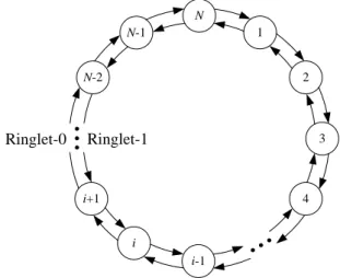
An optical burst switching (OBS) ring contains two unidirectional ringlets and N nodes arranged in the clockwise manner as shown in Fig. 2.1. For simplicity, assume that these N nodes are uniformly distributed on the OBS ring. An OBS node is directly connected with two neighboring nodes, that is, an upstream neighbor and a downstream neighbor. For example, node i is directly connected with node i-1 and i+1 through fiber links. Each node is an ingress node which deals with the packets from the access networks. Here, we consider four service classes: voice, denoted by Vo, video, denoted by Vi, hyper-text transfer protocol (HTTP), denoted by H, and file transfer protocol (FTP), denoted by F. The packet size of the Vo service is fixed with 70 bytes, and each packet size of the other services is uniformly distributed with an variable mean, which ranges from 64 to 1518 bytes.
2 1 N 3 4 i-1 i+1 N-1 N-2 i Ringlet-1 Ringlet-0
8
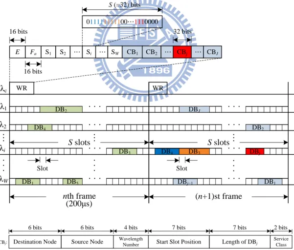
2.1 Slotted OBS Rings
On each ringlet, there are totally (W+1) wavelengths: W data wavelengths and one control wavelength. As shown in Fig 2.2, all the wavelengths are divided into frames, a frame is composed of S slots, and a slot size is 2000-bit long. The data wavelength, denoted by λi, 1 i W, is used for transmitting DBs. The control
wavelength, denoted by λc, contains wavelength reservations (WRs) rotating around
the ring for bandwidth reservation.
The WR comprises of four kinds of messages for the next frame: total empty slots, denoted by E, the advertised fair rate, denoted by Fa, the status of the ith
λ1 λ2 λi λW λc S slots S2 Si … SW Fa WR CB1 CB2 … CBj … S1 … CBJ 011111111100…1110000 S slots WR DBj DB4 DB2 DBJ DB3 DB1 DBj−1 S (=32) bits Slot DB1 DB2 DB3 DB4 DB5 Slot nth frame (n+1)st frame 32 bits (200μs) E 16 bits 16 bits Source Node
Destination Node Wavelength Number Start Slot Position Length of DBj
Service Class
6 bits 4 bits 7 bits 7 bits 2 bits
CBj:
6 bits
9
wavelength, denoted by Si, 1 i W, and the CBj relating to the DBj, 1 j J, where
J is the number of the transit DBs in the next frame. The length of E and Fa are both
16 bits. Note that Fa is used to avoid the congestion and to achieve the fairness
between each node by limiting the amount of the ingress traffic into ringlet, and it is transmitted to upstream nodes. The status of the ith wavelength Si contains S bits, and
each bit represents the status of a corresponding slot in λi at the next frame. An empty
slot is marked as bit “0” and an occupied slot is marked as bit “1.” The CBj comprises
information such as destination node, source node, wavelength number, start slot position, length of DBj in unit of slots, and service class, 1 j J. For simplicity, we
assume that there is no synchronization problem among the wavelengths in every node throughout the thesis.
2.2 Node Architecture
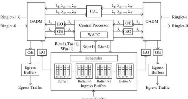
An OBS node, shown in Fig. 2.3, contains two optical add/drop multiplexers (OADMs), four optical-to-electronic (O/E) converters, four electronic-to-optical (E/O) converters, a fiber delay line (FDL), N−1 ingress buffers, some egress buffers, a central processor (CP) with wavelength assignment and traffic control (WATC), and a scheduler. An OADM is used to add traffic to the fiber links at the transmitter or drop traffic from the fiber links at the receiver. Thus, this OBS node can be viewed as that TT-TR architecture is deployed. For simplicity, assume that the wavelength transition time can be ignored. An O/E converts the traffic data from the optical domain to electronic domain, and an E/O converts the traffic data from the electronic domain to optical domain. The FDL is used to delay the transit traffic on data wavelengths to synchronize with the control wavelength with the delay duration about 20~30μs. Ingress buffers and egress buffers are used to temporarily hold the packets for later operations. The WATC helps CP determine how to reserve the empty slots for the
10 Central Processor WATC OADM Egress Buffers Egress Traffic Ingress Traffic O/E Egress Buffers Egress Traffic E/O Ringlet-0 Ringlet-0 Ringlet-1 Ringlet-1 OADM λ1, λ2, ..., λW E/O O/E λc G(n+1) B(n+1), T(n+1), W(n+1) Sa (n+1) FDL λc λc λc O/E E/O E/O λc O/E λc λc λc λ1, λ2, ..., λW λ1, λ2, ..., λW λ1, λ2, ..., λW Ingress Buffers Vi H Buffer 1 Scheduler Vo F Vi H Buffer i–1 Vo F Vi H Buffer i+1 Vo F Vi H Buffer N Vo F
Figure 2.3: Architecture of node i at the nth frame
ingress traffic and to advertise the upstream nodes of traffic limitation in the next frame.
Each node adds its ingress traffic to the ringlet and drops down egress traffic from the ringlet. As for the transit traffic, the node simply bypasses it to next node. The ingress packets are first patched into ingress buffers according to their destinations and are stored in the different queue based on their service classes. Each ingress buffer contains Vo, Vi, H, and F queues. The packets in the same ingress buffer would be assembled into several DBs based on the result of the wavelength assignment by WATC. When the transit DB arrives at its destination, it is disassembled into original packets, which are stored in the egress buffers. Note that a traffic flow means the traffic aggregating in the same source node and destining to the same destination node. Each node deals with traffic on the two ringlets in the same way separately except that the advertised fair rate is sent via the other ringlet. For simplicity, we only illustrate the operations on one ringlet throughout this thesis.
11
2.3 Scheduler
The schedule is used to decide the allowance bandwidth of each queue and its operation is as follows. For example, at the nth frame, the scheduler receives the total available slots for the (n+1)st frame, Sa(n+1), which is calculated by CP. This value is
the maximum number of slots the scheduler can grant. Based on the weighted round robin method [27], the scheduler determines the granted bandwidth of each queue in unit slots in ingress buffers. If no HTTP packet, which is at the head of a queue, exceeds its maximum tolerance delay time, denoted by Td, the weights for the four
traffic types are defined as
Vo : Vi : H : F = : : : , > > > > 0. (2.1)
Otherwise, the weight of the H queue is set to be . Denote the weight of queue j at the nth frame by WEj(n). The granted bandwidth of queue j in unit slots at the (n+1)st
frame is obtained by ( ) ( 1) min ( ), j ( 1) , 1, 2, , 4( 1), j j a WE n g n q n S n j N TW (2.2)
where qj(n) is the length of queue j at the nth frame; represents the floor function,
and the TW is the sum of the total queue weights, 4( 1)
1 ( )
N k k
TW
WE n .The granted bandwidth of all queues is arranged in order of their service classes. For example, gi(n+1), 1 i N−1, represents the granted bandwidth of Vo queue of node i; gi+(N−1)(n+1) is for Vi queue of node i; gi+2(N−1)(n+1) is for H queue of node i;
gi+3(N−1)(n+1) is for F queue of node i. The scheduler generates the granted bandwidth vector, which is defined as
12
1 2 4( 1)
(n 1) g n( 1), g n( 1), g N (n1) , ( g ni 1) S i, 1, 2,...,4(N1).
G (2.3)
This vector is sent to WATC. The WATC will choose appropriate burst sizes to assemble the packets in each queue according to its granted bandwidth. The collection of the length of the assembled DBs is presented by a vector B(n+1) similar as G(n+1), the start time of DBs is presented by a vector T(n+1), and the located wavelengths of DBs is presented by a vector W(n+1). Finally, the WATC marks the status bits of the
nth frame in the WRn by changing related 0’s to 1’s.
2.4 Beforehand Reservation
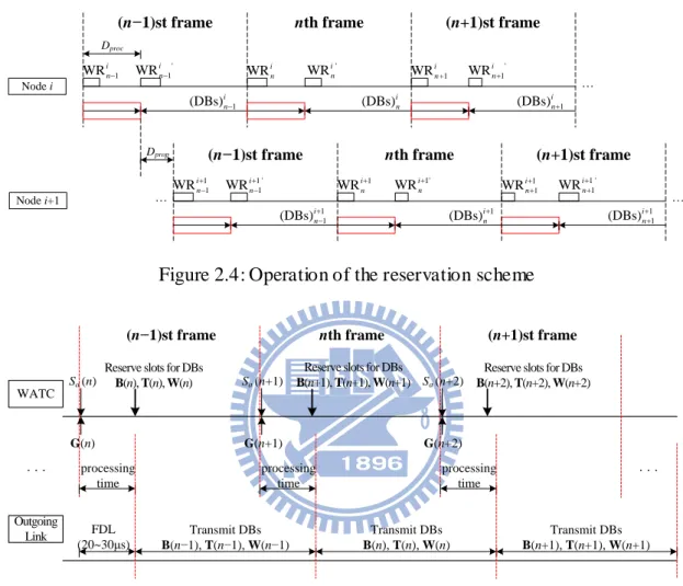
Whenever node i has packets to transmit, it must reserve appropriate slots in advance and then initiate transmissions at the next frame time. Since this is a one-way reservation, no acknowledgement is considered here. Besides, once the DBs are transmitted, their transmission positions cannot be changed by intermediate nodes. The mechanism of beforehand reservation is as follows. At the beginning of the nth frame of node i, WRin is converted to electronic domain and forwarded to CP, shown in Fig. 2.4. After processing the information of WRin, CP determines total available slots Sa(n+1) and sends it to the scheduler. The scheduler would determine the granted
bandwidth G(n+1) immediately and this result would be sent to WATC. Then, WATC chooses appropriate burst size B(n+1), start time T(n+1) of the DBs, and wavelengths
W(n+1), and marks the status bits in the WRin by changing related 0’s to 1’s. The timing sequence in an ingress node is shown in Fig. 2.5. Afterwards, CP discards original WRin and generates WRin', which is sent to the next node. At the same time, the node initiates all the transmissions of DBs, denoted by (DBs)in, that have been reserved at the precious frame. The whole operations continue at every frame time. Note that, the advertised fair rate for current node is sent by the upstream node on the
13
other ringlet. In order to ensure that operations can work normally, the start time of the frames on ringlet-1 differ from those on ringlet-2 half a frame time.
(n−1)st frame nth frame (n+1)st frame
1 WRi n WR 1' i n WRin WR +1 i n ' WRi n ' 1 WRi n Dproc Node i Node i+1 1 ' 1 WRi n WRin1' 1 ' 1 WRi n 1 1 WRi n WRin1 1 1 WRi n
Dprop (n−1)st frame nth frame (n+1)st frame
1 1 (DBs)i n (DBs)in1 1 1 (DBs)i n 1 (DBs)i n (DBs) i n (DBs) 1 i n
Figure 2.4: Operation of the reservation scheme
WATC
Outgoing Link
G(n)
Sa (n)
(n−1)st frame nth frame (n+1)st frame
FDL (20~30μs)
G(n+2)
Sa (n+2)
G(n+1)
Reserve slots for DBs B(n+1), T(n+1), W(n+1)
processing time
Transmit DBs B(n−1), T(n−1), W(n−1) Reserve slots for DBs
B(n), T(n), W(n)
Reserve slots for DBs B(n+2), T(n+2), W(n+2) Transmit DBs B(n), T(n), W(n) Transmit DBs B(n+1), T(n+1), W(n+1) processing time processing time Sa (n+1)
Figure 2.5: Timing sequence in an ingress node
2.5 Fairness Reference Model
In the OBS ring network, when the nodes transmit more data than the link capacity can sustain, an unfair bandwidth allocation problem occurs. The upstream nodes have more chance to transmit their data. In order to achieve fairness bandwidth allocation, some approaches have been proposed for Resilient Packet Ring networks [28], [29]. The concept is to generate an advertised fair rate at each node to regulate
14
transit traffic flows. In order to define the meaning of fairness, an appropriate fairness reference model is important. Here, we adopt the ring ingress aggregated with spatial reuse (RIAS) reference model [30], [31]. In this model, the available bandwidth in current link will be fairly allocated among all ingress aggregated (IA) flows, where IA flow represents the aggregation of all flows originating from a specific ingress node. Furthermore, RIAS ensures maximal spatial reuse. That is, the unused bandwidth can be reallocated to other IA flows while maintaining fairness among the IA flows.
15
Chapter 3
Wavelength Assignment and
Traffic Control (WATC)
3.1 Introduction
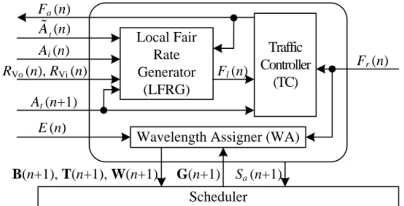
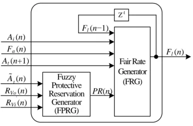
In this thesis, we propose an intelligent wavelength assignment and traffic control (WATC) scheme to determine the wavelengths for ingress traffic and adjust the traffic frame by frame. The WATC scheme consists of a wavelength assigner (WA) to schedule the ingress DBs, a local fair rate generator (LFRG) to generate a local fair rate, denoted by Fl(n), which satisfies the RIAS fairness, and a traffic controller (TC)
to decide an advertised fair rate, denoted by Fa(n), shown in Fig. 3.1. The WA assigns
not only the bandwidth to the queues according to the priority of the traffic but also the proper void to the granted bandwidths of queues as possible. Also, the LFRG would protectively reserve some bandwidth for future voice and video ingress traffic
Traffic Controller
(TC)
Wavelength Assigner (WA)
Fr (n) Fa (n) Local Fair Rate Generator (LFRG) Ai (n) At (n+1) Fl (n) Scheduler G(n+1) B(n+1), T(n+1), W(n+1) Sa (n+1) RVo (n), RVi (n) ( ) t A n E(n)
16
since there is no transit traffic buffer. Finally, the TC generates Fa(n) to inform the
upstream nodes of the traffic limitation for effectively utilizing the bandwidth and enhancing the fairness between nodes. The WATC scheme avoids the bandwidth starvation problem due to no transit traffic buffers and makes better use of link bandwidth in terms of throughput and fairness.
3.2 Wavelength Assigner (WA)
At each nth frame, the WA first computes the total available slots for the (n+1)st frame, Sa(n+1), which could not be reserved at the next frame, at the beginning of nth
frame. The Sa(n+1) can be obtained by
Sa(n+1) = min{E(n+1), Fr(n)}, 0 Sa(n+1) C, (3.1)
where C is the link capacity in unit slots per frame, E(n+1) is the total empty slots at the (n+1)st frame, and Fr(n) is the fair rate received from the downstream nodes. Note
that Fr(n) is obtained from WR on the other ringlet. After the scheduler generates the
granted bandwidth G(n+1) referring to Sa(n+1), the WA will assign the slots to each
queue according to its grated bandwidth. The procedure of wavelength assignment in the WA is shown in Fig. 3.2. For simplicity, the notation of frame time is not shown in the procedure.
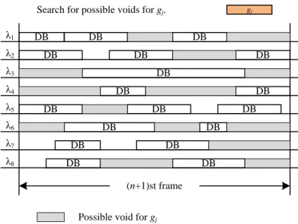
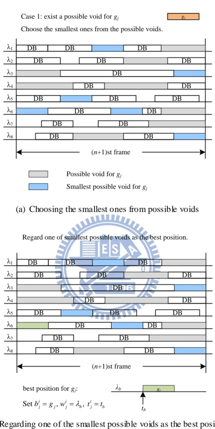
For the value of the (remaining) granted bandwidth of queue j ,denoted by M, the WA searches for possible voids, whose length is longer than gj(n+1), shown in Fig. 3.3. The results are divided into two cases. In case 1, shown in Fig. 3.4 (a), if at least one possible void exists, the WA chooses one of the smallest possible voids as the best position, denoted by (b, t b), for the queue j. As shown in Fig. 3.4 (b), the size of the
17
wavelength assigned for this DB, denoted by w nij( 1), is set as the wavelength on which the best position located, and the start time of this DB, denoted by t nij( 1), is set as that of the best position.
1 to 4( 1)
initialize 1,
( 0)
search for possible voids
(exist a possible void) // case 1 choosed one of the smallest pos
j j N i M g M for while if
sible voids as the best position ( , )
set , , , 0
//case 2
choose the biggest void wit
b b i i i j j b j b t b M w t t M V else
h length as the best position ( , )
set , , , 1, 1 , , V b b i i i j V j b j b V l t b l w t t i i M M l j j end if end while end for return B W T
Figure 3.2: Pseudocode of wavelength assignment
gj DB DB DB DB DB DB DB DB DB λ1 λ2 λ3 λ4 λ5 λ6 λ7 λ8 DB DB DB DB DB DB DB DB DB (n+1)st frame
Possible void for gj
Search for possible voids for gj.
18
gj
Case 1: exist a possible void for gj
DB DB DB DB DB DB DB DB DB λ1 λ2 λ3 λ4 λ5 λ6 λ7 λ8 DB DB DB DB DB DB DB DB DB (n+1)st frame
Possible void for gj
Smallest possible void for gj
Choose the smallest ones from the possible voids.
(a) Choosing the smallest ones from possible voids
DB DB DB DB DB DB DB DB DB λ1 λ2 λ3 λ4 λ5 λ6 λ7 λ8 DB DB DB DB DB DB DB DB DB (n+1)st frame
Regard one of smallest possible voids as the best position.
gj
best position for gj:
tb
λb
Set i , i , i
j j j b j b
b g w t t
(b) Regarding one of the smallest possible voids as the best position
Figure 3.4: Case 1 of WA: (a) choosing the smallest ones from possible voids (b) regarding one of the smallest possible voids as the best position
19
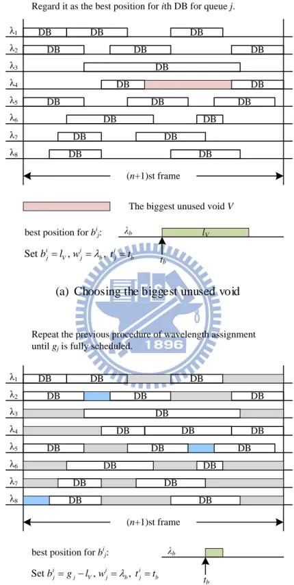
In case 2 as shown in Fig. 3.5 (a), since no possible void exists, it is impossible to generate only one DB for transmitting packets of queue j. Thus, the WA will assign two or more DBs for queue j. First, the WA will choose the biggest void, denoted by V, with length lv as the best position for the first assembled DB of queue j. and sets
( 1)
i j
b n , w nij( 1), and t nij( 1) in the same way as in case 1. In Fig. 3.5 (b), the rest of the granted bandwidth also follows the previous procedure of wavelength assignment and could be categorized into the two cases. The whole wavelength assignment procedure is repeated until each gj(n+1) is appropriate assigned.
The size of each DB, which will be transmitted at the (n+1)st frame, is defined as
1 2 4( 1) (n 1) b n( 1), (b n1), , (b nj 1), , b N (n1) , B (3.2) ( 1) 1 2 ( 1) ( 1), ( 1), , (i 1), , n nj ( 1) , j j j j j b n b n b n b n b n (3.3a) 0 i( 1) ( 1), j j b n g n (3.3b) and it is constrained by ( 1) 1 ( 1) ( 1), j n n i j j i b n g n
(3.4)where b nij
1
is the size of ith DB for queue j, nj(n+1) is the number of DBs for queue j at the (n+1)st frame, 0 nj(n+1) gj(n+1). The start slot position relating to each DB, which will be transmitted at the (n+1)st frame, is obtained by1 2 4( 1) (n 1) t n( 1), (t n1), , (t nj 1), , t N (n1) , T (3.5) ( 1) 1 2 ( 1) ( 1), ( 1), , (i 1), , n nj ( 1) , j j j j j t n t n t n t n t n (3.6a) 1 i( 1) , j t n S (3.6b)
20
gj
Case 2: No possible void for gj
DB DB DB DB DB DB DB DB DB λ1 λ2 λ3 λ4 λ5 λ6 λ7 λ8 DB DB DB DB DB DB DB DB
The biggest unused void V DB
(n+1)st frame
Regard it as the best position for ith DB for queue j.
lV
best position for bij:
tb
λb
Set bjilV, wijb, tijtb
(a) Choosing the biggest unused void
Repeat the previous procedure of wavelength assignment until gj is fully scheduled.
DB DB DB DB DB DB DB DB DB λ1 λ2 λ3 λ4 λ5 λ6 λ7 λ8 DB DB DB DB DB DB DB DB DB (n+1)st frame tb λb
best position for bij:
Set i , i , i
j j V j b j b
b g l w t t
DB
(b) Repeating the previous procedure of wavelength assignment
Figure 3.5: Case 2 of WA: (a) choosing the biggest unused void (b) repeating the previous procedure of wavelength assignment
21
where tij
n1
is the start slot position of ith DB for queue j. The wavelength used by each DB, which will be transmitted at the (n+1)st frame, is obtained by1 2 4( 1) (n 1) w n( 1), w n( 1), , w nj( 1), , w N (n1) , W (3.7) ( 1) 1 2 ( 1) ( 1), ( 1), , i( 1), , n nj ( 1) , j j j j j W n w n w n w n w n (3.8a) 1w nij( 1) W, (3.8b)
where w nij
1
is the wavelength used by ith DB for queue j.Since the length of each void is an integer in the range from 0 to S, the counting sort could be used here, where S is the maximum number of slots on a wavelength per frame. This sorting algorithm takes only θ(X) time at the expense of requiring extra memory, where X is the number of the voids. The binary search algorithm is used to search the possible voids, and it takes the only O(lg X) time. Therefore, the complexity of the total wavelength assignment algorithm is O(X + N lg X), which would be acceptable in the system.
3.3 Local Fair Rate Generator (LFRG)
In order to achieve RIAS fairness mentioned in chapter 2, a traffic control algorithm is proposed. This algorithm is performed frame by frame in each node. The concept is to judge the situations of the link and adjust the fair rate according to observed statistics. As shown in Fig. 3.6, the structure of LFRG contains two parts: fuzzy protective reservation generator (FPRG) and fair rate generator (FRG).
22 Fair Rate Generator (FRG) Fuzzy Protective Reservation Generator (FPRG) Ai (n) At (n+1) Fl (n) PR(n) Z -1 Fl (n−1) Fa (n) RVo (n) ( ) t A n RVi (n)
Figure 3.6: The structure of LFRG
3.3.1 Fuzzy Logic Control System (FLCS)
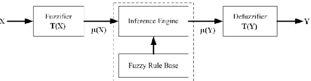
The typical structure of a fuzzy logic control system, shown in Fig. 3.7, comprises of four principal components: a fuzzifier, a fuzzy rule base, an inference engine, and a defuzzifier. The fuzzifier transforms crisp measured input variables X into suitable fuzzy linguistic terms. These fuzzy linguistic terms are specified by membership functions μ(X) and defined in a term set T(X). The fuzzy rule base stores the empirical knowledge, which is described by a collection o f fuzzy control rules (e.g., IF-THEN rules) involving linguistic variables. These rules describe the relationship between the input variable X and the control action Y. The inference engine is the kernel of a FLC. It simulates human decision- making by performing an inference method to yield a desired control, which is described as fuzzy linguistic terms. These fuzzy linguistic terms are specified by membership functions μ(Y) and defined in a term set T(Y). The defuzzifier is used to transform the inferred fuzzy control action to a non- fuzzy control action Y.
23
Figure 3.7: The basic structure of a FLC
3.3.2 Fuzzy Protective Reservation Generator (FPRG)
In the considered network, the transit traffic will bypass current node directly without any O/E and E/O conversions. Therefore, once the frame is fully used by upstream nodes, current node would hardly have bandwidth to transmit its own data, even if the service class of the data is more important than those of the transit traffic. Although this problem can be alleviated by the advertised fair rate, it takes much propagation time to see the effect. In order to further alleviate the mentioned problem, we protectively reserve some bandwidth, denoted by PR(n), in advance for future voice and video traffic in ingress nodes.
Here, a fuzzy inference system is used to determine the protective reservation. FPRG has three inputs: the moving average of transit traffic, denoted by A nt( ), the ratio of moving average of voice transit traffic to moving average of total transit traffic at the nth frame, denoted by RVo(n), and the ratio of moving average of video transit traffic to moving average of total transit traffic at the nth frame, denoted by
RVi(n). A nt( ) is obtained by 1 1 ( ) ( ), n t t k n L A n A k L
(3.9)24
observation window. In other words, A nt( ) is a moving average of At(n). RVo(n) and
RVi(n) is obtained by ( ) ( ) , 0 ( ) 1, ( ) Vo t Vo Vo t A n R n R n A n (3.10) ( ) ( ) , 0 ( ) 1, ( ) Vi t Vi Vi t A n R n R n A n (3.11)
respectively, where AtVo
n is the arrival rate of voice transit traffic in unit slots atthe nth frame, AtVi
n is the arrival rate of video transit traffic in unit slots at the nthframe. The output of FPRG is PR(n), which is the protective reservation in unit slots at the nth frame for future voice and video traffic in the ingress node.
We define the term set for A nt( ) as T(A nt( )) = {Low (L), Medium (M), High (H)}; for RVo(n) as T(RVo(n)) = {Low (L), High (H)}; for RVi(n) as T(RVi(n)) = {Low (L) , Medium (M), High (H)}; for RVi(n) as T(RVi(n)) = {Low (L) , Medium (M), High (H)}.
We use the triangular function f(x; x0, a0, a1) and the trapezoidal function g(x; x0,
x1, a0, a1) to define the membership functions for terms in the term set. These two functions are given by
0 0 0 0 0 0 0 0 1 0 0 1 1 1, if , ( ; , , ) 1, if , 0, otherwise, x x x a x x a x x f x x a a x x x a a (3.12) and
25 0 0 0 0 0 0 1 0 1 0 1 1 1 1 1 1 1, if , 1, if , ( ; , , , ) 1, if , 0, otherwise, x x x a x x a x x x g x x x a a x x x x x a a (3.13)
where x0 in f(·) is the center of the triangular function; x0 (x1) in g(·) is the left (right) edge of the trapezoidal function; a0 (a0) is the left (right) width of the triangular or the trapezoidal function. The center, edge, or width of the triangular or trapezoidal membership function is set intuitively but based on the characteristics of the linguistic variables.
The corresponding membership functions of L, M, and H in T( A nt( )) are denoted as ( ( )) ( ( );0, 0.45 , 0, 0.2 ), L A nt g A nt C C (3.14) ( ( )) ( ( );0.65 , 0.2 , 0.2 ), M A nt f A nt C C C (3.15) ( ( )) ( ( ); 0.85 , , 0.2 , 0), H A nt g A nt C C C (3.16)
where C is the channel capacity in unit slots. The corresponding membership functions of L and H in T(RVo(n)) are denoted as
( ( )) ( ( );0, 0.3, 0, 0.2), L RVo n g RVo n (3.17) ( ( )) ( ( );0.5, 1, 0.2, 0). H RVo n g RVo n (3.18)
The corresponding membership functions of L, M, and H in T(RVi(n)) are denoted as
( ( )) ( ( );0, 0.2, 0, 0.2), L R nVi g R nVi (3.19) ( ( )) ( ( );0.4, 0.5, 0.2, 0.2), M R nVi g R nVi (3.20)
26
( ( )) ( ( );0.7, 1, 0.2, 0).
H R nVi g R nVi
(3.21)
For the reason of simplicity in computation of defuzzification, let the membership functions for Null (Nu), Very Low (VL), Low (L), Medium (M), High (H), Very High (VH) in T(PR(n)) be fuzzy singletons. Define these membership functions as
( ( )) ( ( ); 0, 0, 0). Nu PR n f PR n (3.22) ( ( )) ( ( ); 10, 0, 0), VL PR n f PR n (3.23) ( ( )) ( ( ); 20, 0, 0), L PR n f PR n (3.24) ( ( )) ( ( ); 30, 0, 0), M PR n f PR n (3.25) ( ( )) ( ( ); 40, 0, 0), H PR n f PR n (3.26) ( ( )) ( ( ); 50, 0, 0). VH PR n f PR n (3.27) 0.10.20.3 0.40.50.60.70.8 0.9 1 0 (RVo( ))n ( ) Vo R n ( ) (A nt ) C (R nVi( )) ( ) Vi R n 10 20 30 40 50 0 (PR n( )) ( ) PR n ( ) t A n C VH VL H H H H L L L L M M Nu M 1 1 1 1 0.10.20.3 0.40.50.60.70.8 0.9 1 0 0.10.20.3 0.40.50.60.70.8 0.9 1 0 (a) (b) (c) (d)
Figure 3.8: The membership functions of the term set (a) T(RVo(n)) (b) T(RVi(n)) (c)
27 Rule A n t
RVo (n) RVi (n) PR(n) Rule A n t
RVo (n) RVi (n) PR(n) 1 L L L L 10 M H L L 2 L L M L 11 M H M L 3 L L H VL 12 M H H VL 4 L H L VL 13 H L L VH 5 L H M Nu 14 H L M VH 6 L H H Nu 15 H L H H 7 M L L H 16 H H L H 8 M L M M 17 H H M M 9 M L H M 18 H H H MTable 3.1: The rule base of FPRG
The membership functions of T(PR(n)) are discrete uniformly distributed between 0 and 50. All membership functions of FPRG are shown in Fig. 3.8.
The rule base of FPRG is shown in Table 3.1. The order of significance of the input linguistic is A nt( ), RVo(n), and then RVi(n). When the arrival rate of transit traffic is high, the protective reservation would be set high to prevent the voice and video ingress traffic from bandwidth starvation. And if the important portion of the transit traffic, including voice and video traffic, is relatively low, the protective reservation would be set higher, too.
The FPRG adopts the max- min inference method for inference engine. To explain max- min inference method, we consider rule 5 and rule 6 which have the same control action “PR(n) is Nu.” Applying “min” operator, we obtain the membership function values of the control action “PR(n) is Nu” of rule 5 and rule 6 respectively by
5( ) min{ L( t( )), H( Vo( )), M( Vi( ))},
m n A n R n R n (3.28)
6( ) min{ L( t( )), H( Vo( )), H( Vi( ))}.
28
Then, applying the “max” operator, the overall membership value of the control action “PR(n) is Nu” , denoted as wNu(n), is obtained by
5 6
( ) max{ ( ), ( )}.
Nu
w n m n m n (3.30)
Similarly, the overall membership function of the control action VL, L, M, H, and VH, denoted as wVL (n), wL (n), wM (n), wH (n), and wVH(n), respectively, can be obtained. After inferring all the rules, FPRG uses center of area (COA) method for defuzzifier. The output value PR(n) is obtained by
0 ( ) 10 ( ) 20 ( ) 30 ( ) 40 ( ) 50 ( ) ( ) . ( ) ( ) ( ) ( ) ( ) ( ) Nu VL L M H VH Nu VL L M H VH w n w n w n w n w n w n PR n w n w n w n w n w n w n (3.31)
3.3.3 Fair Rate Generator (FRG)
Here, we define a parameter, denoted by M(n), to measure the equivalent number of IA transit flows traversing node i , whose rate is equal to previous advertised fair rate. This parameter is determined by
( ) ( ) ( ) , ( 1) i t a A n A n M n F n (3.32)
where Ai(n) is the arrival rate of ingress traffic in unit slots at the nth frame,
4( 1) 1
( ) min ( ( ), N ( )).
i r j j
A n F n
q n , qj(n) is the length of queue j at the (n+1)st frame;( 1)
a
F n is the moving average of Fa(n−1), which is the advertised fair rate
generated at the (n–1)st frame, F na( 1) (1/ )L
k n Ln 1 F ka( ). The local fair rate at the nth frame is calculated as29 1 ( ) min ( ), ( 1) ( ( ) ( ( ) ( 1))) , ( ) l l i t F n C PR n F n C PR n A n A n M n (3.33)
where PR(n) is the protective reservation in unit slots at the nth frame for future voice and video traffic in ingress node.
3.4 Traffic Controller (TC)
The traffic condition in the fiber link is always changing. In order to alleviate the overuse of a link as well as make better use of the link capacity, TC is design to adapt the IA flows. In order to decide the traffic condition, TC observes the incoming transit traffic, say At(n+1), and compares it with the minimum of the local fair rate Fl(n) and
the received advertised fair rate from the other ringlet, called Fr(n). The main reason
of using minimum operation is to be a little more conservative in order not to incur overuse of a link too often. Depending on the traffic conditions, TC takes two possible actions.
3.4.1 Traffic Suppression
If At(n+1) is bigger than or equal to the minimum of Fl(n) and Fr(n), the link is
considered as overused. So, TC will decrease the rates of IA flows, and choose the minimum of Fl(n) and Fr(n) as the advertised fair rate Fa(n).
3.4.2 Traffic Promotion
If At(n+1) is smaller than or equal to the minimum of Fl(n) and Fr(n), the link is
considered as not sufficiently used. So, TC will increase the rates of IA flows, and choose the maximum of Fl(n) and Fr(n) as the advertised fair rate Fa(n).
30
Chapter 4
Simulation Results
4.1 Simulation Environment
In the simulations, the general settings for environment include link capacity of 10Gbps, 7 data wavelengths, one control wavelength, 200μs propagation delay between nodes, 200μs frame time, and 1.6μs slot time. In terms of unit slot which is 2.5k bits, the link capacity per frame (C) is 875 slots and the number of slots per data wavelength in a frame (S) is 125. All the simulation parameters are listed in Table 4.1. The network traffic includes four service classes, each occupies one fourth of the total amount. Simulation results are recorded per frame time to show the bandwidth usage on an overused link.
The wavelength assignment of WATC scheme is compared to OBS-GS [21]. The OBS-GS groups the DBs in a collecting period, and assigns them proper positions to maximize the link utilization. It is assumed that the DBs scheduled by OBS-GS are generated using the volume-based burst assembly algorithm. For simplicity, the traffic scenario is assumed homogeneous, which means that each node generates equal amount of traffic, and the nodes are all greedy. On the other hand, the performance of the traffic control of the WATC scheme is compared to DBA [28]. The DBA estimates the equivalent number of IA flows referring to current arriving traffic and allocate the residual bandwidth equally to these IA flows.
31 Circumference of ring 200 km 320 km Number of nodes (N) 5 8 Node architecture TT-TR Link capacity 10 Gbps Light velocity 2×10⁸ m/s
Number of data channels (W) 7
Number of control channels 1
Frame time 200 μs
Number of slots per frame per wavelength (S) 125
Slot time 1.6 μs
Link capacity per frame in unit slots (C) 875 slots
Weights of four service classes: voice, video, HTTP, FTP
{α, β, γ, δ}={4, 3, 2, 1}
Table 4.1: General settings for environment
4.2 Comparisons of Wavelength Assignment Methods
In this section, simulations are conducted to compare the performances of the wavelength assignment of the WATC scheme with OBS-GS. Figure 4.1(a) shows a large parking lot scenario where there are eight greedy nodes. This scenario assumes that the flows are generated from node 1, 2, 3, 4, 5, 6, and 7 but terminated at node 8. The simulated traffic is homogeneous and composes of four service classes. Cooperating with the traffic control of the WATC scheme, the total throughputs of the two wavelength methods, denoted by WATC and OBS-GS_TC, are shown in Fig.
32
4.1(b). The throughputs recorded are in the outgoing link of node 7, and they are normalized to the link capacity. It can be seen that the throughput of the WATC scheme approximate the link capacity. However, the throughput of the OBS-GS_TC scheme only achieves 95% of the link capacity. This is due to the fact that OBS-GS only searches and utilizes the earliest possible voids. Whenever a granted queue has no possible void to put on its data, OBS-GS would leave the data behind and wait for reservation next time. Instead, the WA would divide the granted queue into two smaller pieces of data and assign each of them an approximate void, thus the WATC scheme has better performance.
Node 1 Node 2 Node 3 Node 4 Node 5 Flow(4-8)
Flow(5-8)
Flow(6-8)
Flow(7-8)
Node 6 Node 7 Node 8 Flow(1-8)
Flow(2-8)
Flow(3-8)
Node N
Figure 4.1(a): Large parking lot scenario with homogeneous traffic
0.8 0.85 0.9 0.95 1 1.05 1.1 1.15 1.2 0 10 20 30 40 50 60 70 80 90 N o r m a li z e d T o ta l T h r o u g h p u t Time (msec) WATC OBS-GS_TC
33
Alternatively, the throughputs of the two wavelength methods cooperating with DBA, denoted by WA_DBA and OBS-GS_DBA, are shown in Fig. 4.1(c). It is found that the wavelength assignment of the WATC scheme also has high throughput. Unfortunately, the OBS-GS_DBA not only has lower throughput, but also suffers from throughput oscillation. This reveals the disad vantage of DBA, that is, the flows can hardly converge in many scenarios. The oscillation makes the available bandwidth time-varying. Besides, OBS-GS cannot fully utilize these bandwidth and further worse the oscillation. Therefore, the curve of the oscillation is not smooth. Obviously, the wavelength assignment of the WATC scheme is better than OBS-GS for OBS ring networks.
0.8 0.85 0.9 0.95 1 1.05 1.1 1.15 1.2 0 10 20 30 40 50 60 70 80 90 N o r m a li z e d T o ta l T h r o u g h p u t Time (msec) WA_DBA OBS-GS_DBA
Figure 4.1(c): The normalized throughputs of WA_DBA and OBS-GS_DBA
4.3 Comparisons of Traffic Control Methods
4.3.1 Homogeneous Traffic Generated by Constant-bit-rate Traffic
Pattern
34
nodes. Figures 4.2(b) and 4.2(c) present the normalized throughput of each flow in the outgoing link of node 4 controlled by WATC and WA_DBA. This scenario assumes that flows are generated from node 1, 2, 3, and 4 but terminated at node 5. The propagation delay is small. The simulated traffic includes four service classes, but only the HTTP and FTP traffic are controlled to meet the fairness. The throughputs are normalized to the link capacity. These flows all start at 0 ms. As shown in Figs. 4.2(b) and 4.2(c), the flows of WATC and WA_DBA take 17 and 26.4 ms to become stable, respectively. The WATC improves the convergence time over the WA_DBA by 35.6%. It is due to the fact that the WA_DBA generates the fair rate to regulate the flows of upstream node referring to the short-term arriving traffic, but it takes some propagation time to see the actual influence of each adjustment of the advertised fair rates. This would incorrectly limit the amount of the transit traffic to the next node and cause the WA_DBA to make an error decision. As a result, the WA_DBA may adjust the flows too much, incurring a longer convergence time. On the contrary, the WATC calculates the moving average of arriving traffic within an observation window to mitigate the effect of propagation delay. This can avoid rapid flow adjustment and thus improve the convergence time.
In Fig. 4.2(b), it is found that the Flow(4-5) has slightly more throughput than the other flows. This is due to the fact that the WATC scheme applies the protective reservation, which allows the ingress node have more bandwidth for its voice and video traffic. The difference between the Flow(4-5) and the other traffic flows is only the throughput of voice and video traffic. The amount of the protective reservation is dynamically generated the FPRG according to the network conditions. It can also be observed that, at steady state, the throughputs of all flows are approximately the same as required, thus achieving fairness.
35
Node 1 Node 2 Node 3 Node 4 Node 5
Flow(1-5)
Flow(2-5)
Flow(3-5)
Flow(4-5) Node N
Figure 4.2(a): Small parking lot scenario with homogeneous traffic
0 0.05 0.1 0.15 0.2 0.25 0.3 0.35 0.4 0.45 0.5 0 10 20 30 40 50 60 70 80 90 N o r m a li z e d T h r o u g h p u t Time (msec) Flow(1-5) Flow(2-5) Flow(3-5) Flow(4-5)
Figure 4.2(b): The normalized throughputs of WATC
0 0.05 0.1 0.15 0.2 0.25 0.3 0.35 0.4 0.45 0.5 0 10 20 30 40 50 60 70 80 90 N o r m a li z e d T h r o u g h p u t Time (msec) Flow(1-5) Flow(2-5) Flow(3-5) Flow(4-5)
36
In Figs. 4.2(b) and 4.2(c), it is found that the oscillation of Flow(4-5) is different from the other flows. The Flow(4-5) increases when the other flows decreases and vice versa. The reason is that the node architecture does not have transit buffers, thus the node 4 can use only the residual bandwidth after node 1 to node 3 have reserved their bandwidth. Besides, since the overused link occurs at the outgoing link of node 4, all the flows from upstream nodes are regulated by the fair rate generated by node 4 and being changed in turn.
Figure 4.3(a) shows a large parking lot scenario where there are eight greedy nodes. Figures 4.3(b) and 4.3(c) present the normalized throughputs of Flow(1-8), Flow(3-8), Flow(5-8), and Flow(7-8) in the outgoing link of node 7 controlled by WATC and WA_DBA. This scenario assumes that flows are generated from node 1, 2, 3, 4, 5, 6, and 7 but terminated at node 8. Again, only the HTTP and FTP traffic are controlled to meet the fairness, and the throughputs are normalized to the link capacity. These flows all start at 0 ms. In Fig. 4.3(b), it can be seen that the flows of WATC take21 ms to become stable. Unfortunately, it is hard for WA_DBA to make the flows become stable. This is due to the fact that the WA_DBA computes the number of effective IA flows referring to both the short-term traffic and the previous local fair rate to generate the current local fair rate. However, due to the large propagation delay, the correlation between the short-term traffic and the previous local fair rate becomes low. Therefore, the WA_DBA cannot generate a correct local fair rate to regulate the flows. As a result, the flows oscillate and barely converge.