極化式編碼於孔徑函數上之應用

國立交通大學

光電工程研究所

碩士論文

極化式編碼於孔徑函數上之應用

Polarization Coded Aperture Engineering

研 究 生：鍾議寬

指導教授：田仲豪 副教授

極化式編碼於孔徑函數上之應用

Polarization Coded Aperture Engineering

研 究 生：鍾議寬 Student:Yi-Kuan Chung

指導教授：田仲豪 Advisor:Chung-Hao Tien

國立交通大學

光電工程研究所

碩士論文

A Thesis

Submitted to Department of Photonics College of Electrical and Computer Engineering

National Chiao Tung University in partial Fulfillment of the Requirements

for the Degree of Master

in

Department of Photonics

July 2010

Hsinchu, Taiwan, Republicof China

i

極化式編碼於

孔徑函數上之應用

碩士研究生：鍾議寬 指導教授：田仲豪

國立交通大學

光電工程研究所

摘要

繞射理論可依據觀測材料的特性與觀測維度的大小，分成將電磁場視為純量 的純量繞射理論與實際考量各點邊界條件解出該點電磁場，計算上較為複雜的向 量繞射。以往，於空間解析度低的情況下(低數值孔徑)，採用純量繞射已可得到 不錯的近似解；然而，由於科技的日益進步，空間解析度也日漸增加(高數值孔 徑)，光的向量特性必須加以考量，此時純量繞射已不再適用，必須採用向量繞 射來解釋。 因此，於此篇論文中，首先會針對各種極化於聚焦平面上的場形分布做討論， 指出不同極化於高數值孔徑的系統下，聚焦場形之各種特性。接著，考量到極化 於日後顯微系統的影響，我們利用不同或高階數的非勻質極化於孔徑上的分布， 來達到拓展景深的應用；之後再藉由創造出的多波長非勻質極化光，將其應用至 表面電漿領域，建立一個即時之感測系統，並提出一金屬-絕緣層-金屬的結構， 來完善此感測系統。

ii

Polarization Coded Aperture Engineering

Master student: Yi-Kuan Chung Advisor: Dr. Chung-Hao Tien

Institute of Electro-Optical Engineering

National Chiao Tung University

Abstract

In the diffraction theory, scalar diffraction theory is based on specific material

condition or observed with low NA system, the fields are treated as the scalar

components to obtain a good approximation by relatively simple mathematics formula.

However, while the technique was fast developed, the dimension and materials is

more and more small and variety, respectively. Therefore, the vetorial properties of

light are no longer neglected in the discussion of polarization.

In this thesis, first part was addressed about the effect of polarization in

different numerical apertures, the influence of polarization is more distinct as

numerical aperture increases. The second part was addressed to discuss extending

depth of focus by the synthesis of polarizations. The third part is to build up a

polychromatic SPR sensor system utilized excited chromatic radially polarized light

iii

誌謝

首先感謝指導教授 田仲豪老師兩年來在研究上給予的指導、並時常分享學 習上以及人生經歷上的寶貴經驗，讓我除了能夠順利完成學業及此論文外，也了 解到很多待人處事上該有的態度。 還必須感謝的是實驗室中帶領我一步一步學習到畢業的子翔學長，還有給予 許多關於學習相關經驗的小陸學長、健翔學長、進哥學長、壯哥學長。以及一起 努力到畢業的同伴鍾岳，在研究的路途上，因為有你們的陪伴使我能夠更順利地 走完這趟學習之路。同時感謝實驗室的杰恩學弟、國恩學弟、孟潔學妹，希望明 年你們也能順利畢業。額外感謝益智學長在玩樂時間的陪伴。 再來感謝我的家人，從小栽培我到大，能夠讓我無後顧之憂地完成學業，並 永遠支持著我，也感謝我的女朋友，能夠體諒我因為研究而無法時常陪伴在她身 邊，並分擔著我的煩惱與憂愁，最後也感謝其他的朋友們，因為你們，讓我在學 習的路上並不孤單，在此，將畢業的喜悅分享給大家。

iv

Table of Contents

Abstract(Chinese) ………..………..……..…..…i

Abstract(English) ………...…….…...….ii

Acknowledgement ...………..….………....iii

Table of Contents ……….…….…..…....…iv

Figure Captions ...………..………..……...…..…v

List of tables ………viii

Chapter 1 Introduction………...…………..1

1.1 Scalar diffraction theory………..1

1.1.1 Kirchhoff diffraction formula………..…..2

1.1.2 Fresnel-Kirchhoff diffraction formula....……….4

1.1.3 Rayleigh-Sommerfeld diffraction formula………..5

1.2 Vector diffraction theory………..7

1.2.1 Vectorial Debye theory…….………..…..7

1.2.2 Fresnel’s equations……….………..…..7

1.2.3 Jones calculus………..……….9

1.3 Comparison of two diffraction theory………11

1.4 Motivation & Organization………11

Chapter 2 Polarization Beams………...………….16

2.1 Homogeneous and inhomogeneous polarization………16

2.2 Properties of polarized beam………..17

2.2.1 Linear polarization………..………..…….17

2.2.2 Circular polarization………..……….19

2.2.3 Radial polarization………..20

2.2.4 Azimuthal polarization………21

2.3 Summary………21

Chapter 3 Application 1 – Extended Depth of Focus………23

3.1 History and Principle………….……….23

3.2 Combination of inhomogeneous beams…...………..27

3.3 Higher-order radially polarized beam………32

v

Chapter 4 Application 2 – Chromatic Surface Plasmon Resonance…35

4.1 History and Principle ………….……….…………35

4.2 Experimental Setup……….…………39

4.2.1 Synthesis of radially polarized white light……….41

4.2.2 MIM Structure………..42

4.3 Matrix method……….44

4.4 Simulation and Experimental Data……….46

4.5 Summary………..………...…….51

Chapter 5 Conclusions and Future work………52

5.1 Conclusions………..………...…52

5.2 Future work………..………...…53

Reference……….54

Figure Captions

Fig. 1-1 Slice through the volume V. ……….3

Fig. 1-2 A plane screen with point-source illumination. ……….……..4

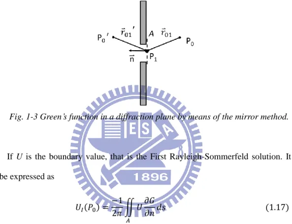
Fig. 1-3 Green’s function in a diffraction plane by means of the mirror method. …....6

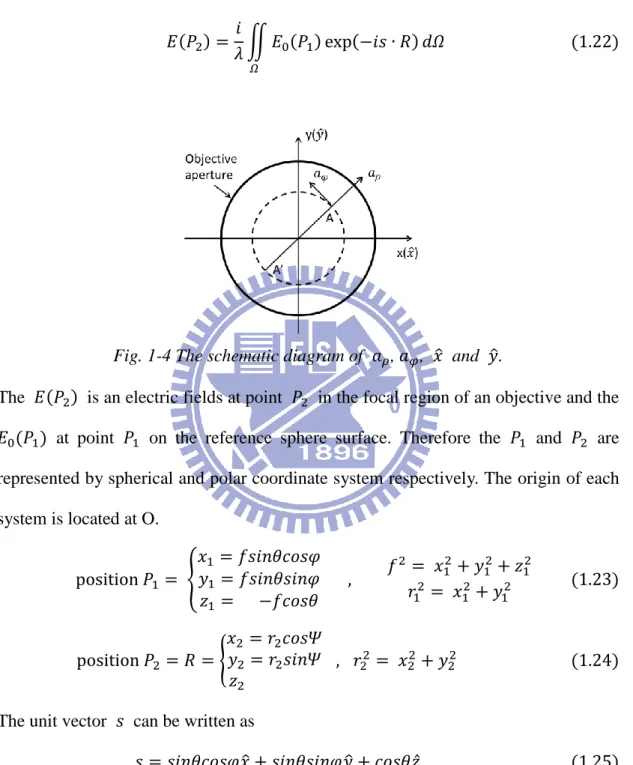
Fig. 1-4 The schematic diagram of a_ρ, a_φ, x̂ and ŷ. ……….….………....8

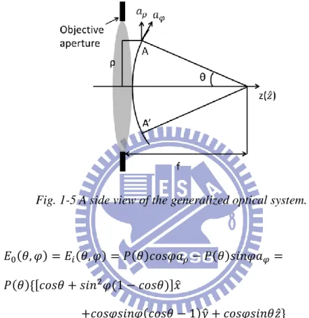
Fig. 1-5 A side view of the generalized optical system. ………9

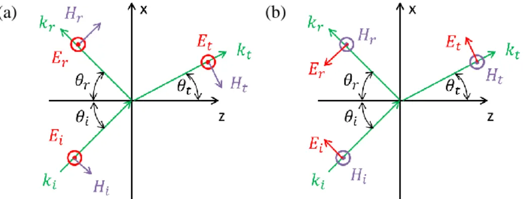
Fig. 1-6 Geometry of Fresnel’s equations for (a) s-polarization and (b) p-polarization. ………..………...10

Fig. 2-1 (a) and (b) illustrates the homogeneous and in homogeneous beam, respectively. ……….16

Fig. 2-2 Intensity distribution of the cylindrical vector beams. (a) Radial (b) Azimuthal polarization. ………...………17

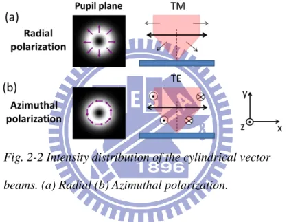
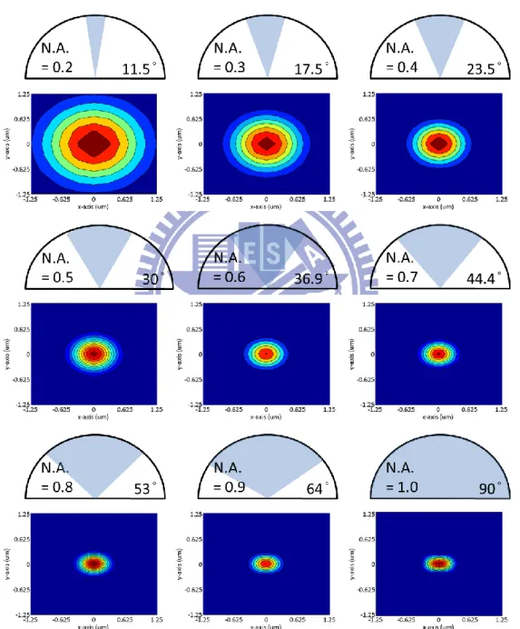
Fig. 2-3 Intensity profile of linearly polarized focus as numerical aperture increases from 0.2 to 1.0, where the vectorial feature becomes more apparent with high-NA system. ………..………...18

vi

Fig. 2-4 Intensity profile of circular polarized focus for increasing numerical

aperture. ………...…19

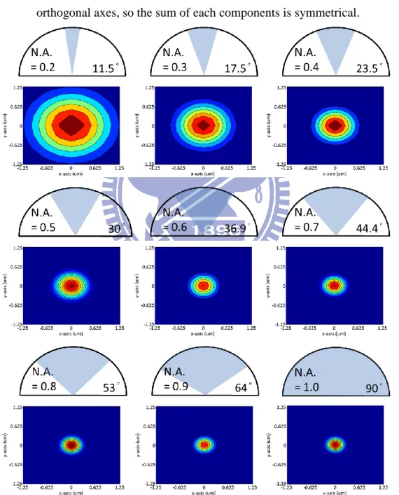
Fig. 2-5 Intensity profile of radially polarized beams in different numerical aperture.

When numerical aperture increased, the optical field is transformed from a

doughnut-shaped to a flat-topped shape. ……….21

Fig. 2-6 Focused intensity profile of azimuthally polarized beams for high numerical

aperture. ………..….21 Fig. 2-7 Each component of focal fields in azimuthally polarized light, due to the

destructive interference of depolarization effect, the electric field of z-component is

zero. ………..….………...….22 Fig. 3-1 The configuration for annular aperture. ………...25

Fig. 3-2 The schematically concept of extending depth of focus by refractive

optics. .…...………..26

Fig. 3-3 The polarization coded aperture.………27

Fig. 3-4 Two types of radial and azimuthal combination. ………...28

Fig. 3-5 (a) to (j) peak intensity across different z-axis position when radially

polarized light is in outer ring region. ……….……….………...29

Fig. 3-6 (a) to (j) peak intensity across different z-axis position when azimuthally

polarized light is in outer ring region. ……….30

Fig. 3-7 The FWHM of (a) radially polarized light and (b) azimuthally polarized light

focal fields. ………..31 Fig. 3-8 The intensity profile comparison between linear polarization coded aperture

and in homogeneous coded aperture on x-y dimension. ……….31

Fig. 3-9 The fundamental mode (R-TEM01) and two higher-order modes (R-TEM11

and R-TEM21) of radially polarized beam. ………..………...….32

vii

Fig. 4-1 (a) s-polarization (b) p-polarization waves propagate between two media. ..36

Fig. 4-2 configuration of the PC-RPSPR sensor, where CL: collimated lens, SVP:

spatial varying polarizer, RL: relay lens, BS: beam splitter, IL: image lens, MIM:

metal-insulator-metal structure. The insets show (a) the photo of SVP, (b) the

schematic diagram of MIM structure. ………...…….….40

Fig. 4-3 The SVP assembly, which is composed of eight sectors. ...………...………41

Fig. 4-4 Comparison with the different test sample. (a) and (c) are experimental data

and (b) and (d) are simulation when test sample is air and water, respectively.(e) and

(f) are the slice of (b) and (d), respectively. The wavelength here is 610 nm. ……43

Fig. 4-5 Obviously angular shift in T-SPR modes by comparing the different

refractive index of test sample. ………44

Fig. 4-6 Geometry for propagation matrix. ……….45

Fig. 4-7 Schematic drawing showing the matrix method. ……….…..46

Fig. 4-8 Radially polarized white light generated by radial polarizer. The arrows

indicate the axis direction of analyzer. ……….………...47

Fig. 4-9 The (a) experimental and (b) simulated observation of reflected rainbow disk

for the case of free space in contact with the gold monolayer structure, where

subfigures 1 to 3 are respectively show the dark resonance ring observed at

wavelength λ = 610 nm, 530 nm, and 450 nm. ………...48

Fig. 4-10 comparison shows the effect of MIM structure (λ=610nm). ……...………49

Fig. 4-11 (a) rainbow concentric ring in different sensing condition (b) the spectra

distribution of rainbow concentric rings as the medium above the MIM structure is

chosen saline with different concentration. ……….50

viii

List of Table

Table 1-1 The reference between polarization and Jones vector. ………12

1

Chapter 1

Introduction

Diffraction denotes the deviation of light rays from rectilinear propagation

which cannot be interpreted by either refraction or reflection. The diffraction theory

can be divided into two parts which is based on solving the boundary condition

problem or not. In this chapter, we will introduce two diffraction theories, then

compare to each other.

1.1 Scalar diffraction theory

Classical scalar diffraction theory does not solve the boundary condition

problem but a boundary value problem; it means that scalar diffraction theory is able

to describe diffraction of light via a simple mathematical formula, because the

hypotheses of material lead to all components of the electric and magnetic field

having identical behavior which is fully described by a single scalar wave equation

[1].

If the propagation medium is linear, isotropic, homogeneous, non-dispersive,

nonmagnetic, then applying the ∇ × operation to the Maxwell equation 𝛻 × (𝛻 × 𝐻⃑⃑ ) = 𝜀𝑑(𝛻 × 𝐸⃑ )

𝑑𝑡 (1.1a) 𝛻 × (𝛻 × 𝐸⃑ ) = −𝑢𝑑(𝛻 × 𝐻⃑⃑ )

𝑑𝑡 (1.1b) 𝛻 × (𝛻 × 𝑢⃑ ) = 𝛻(𝛻 ∙ 𝑢⃑ ) − 𝛻2_{𝑢⃑ (1.1c)}

Where u represents any of the vector field components, substitution of the Eq. (1.1a)

and Eq. (1.1b) in Eq. (1.1c) yields

𝛻2_{𝐻⃑⃑ −}𝑛2

𝑐2

𝜕2_𝐻⃑⃑

2

𝛻2_{𝐸⃑ −}𝑛2

𝑐2

𝜕2_𝐸⃑

𝜕𝑡2 = 0 (1.2b)

Where n is the refractive index of the medium, defined by

𝑛 = (𝜀 𝜀₀) 1 2 ⁄ (1.3𝑎) And c is the velocity of propagation in vacuum, written as

𝑐 = 1 √𝜇0𝜀0

(1.3𝑏) Since the Eq. (1.2a) and Eq. (1.2b) can apply for both electric and magnetic field,

therefore, it is possible to summarize the behavior of all components of electric and

magnetic field through a single scalar wave equation

𝛻2_{𝑢(𝑃, 𝑡) −}𝑛2

𝑐2

𝜕2_{𝑢(𝑃, 𝑡)}

𝜕𝑡2 = 0 (1.4)

Where 𝑢(𝑃, 𝑡) represents any scalar field components of electric and magnetic field, and the components dependent on both position P in space and time t.

From above we assume that propagation medium is linear, isotropic,

homogeneous, non-dispersive, nonmagnetic, then we can treat the electric and

magnetic field as a scalar field to simplify the behavior of diffraction. The scalar

diffraction theory is well known as Fourier optics.

1.1.1 Kirchhoff diffraction formula

The Kirchhoff diffraction formula is a solution of the scalar, time-independent

wave equation using Green’s relation

∭(𝑈(𝑃)𝛻2_{𝐺(𝑃) − 𝐺(𝑃)𝛻}2_𝑈(𝑃)) 𝑉 𝑑𝑣 = ∯ (𝑈(𝑃)𝜕𝐺(𝑃) 𝜕𝑛 − 𝐺(𝑃) 𝜕𝑈(𝑃) 𝜕𝑛 ) 𝑆=𝑆1+𝑆2 𝑑𝑠 (1.5)

3

direction at each point on S. U(P) and G(P) are any function of position. As shown in

Fig. 1-1

Fig 1-1 Slice through the volume V.

If U and G both satisfy the free-space Helmholtz equation.

(𝛻2_{+ 𝑘}2_{)𝐺 = 0 (1.6𝑎)}

(𝛻2_{+ 𝑘}2_{)𝑈 = 0 (1.6𝑏)}

Substituting the Eq. (1.6a) and Eq. (1.6b) in the Eq. (1.5), we obtain

∯ (𝑈𝜕𝐺 𝜕𝑛− 𝐺 𝜕𝑈 𝜕𝑛) 𝑆=𝑆1+𝑆2 𝑑𝑠 = 0 (1.7) Choosing a spherical wave as an auxiliary function expanding at the point P0, then the

value of G at arbitrary point P1 is given by

𝐺(𝑃₁) =𝑒𝑥𝑝(𝑖𝑘𝑟01) 𝑟₀₁ And 𝜕𝐺(𝑃1) 𝜕𝑛 = cos (𝑛⃑ , 𝑟 01)(𝑖𝑘 − 1 𝑟01) 𝑒𝑥𝑝(𝑖𝑘𝑟01) 𝑟01 (1.8)

Where 𝑟₀₁ is the length of vector 𝑟 ₀₁ pointing from P0 to P1. For a particular case of

P1 on S2, cos(𝑛⃑ , 𝑟 01) = −1, the Eq. (1.8) become

𝐺(𝑃₁) =𝑒𝑖𝑘𝜀_𝜀 𝑎𝑛𝑑 𝜕𝐺(𝑃1) 𝜕𝑛 = ( 1 𝜀− 𝑖𝑘) 𝑒𝑖𝑘𝜀 𝜀 (1.9) Letting 𝜀 is tending to zero, then

4 lim 𝜀→0∬ (𝑈 𝜕𝐺 𝜕𝑛 − 𝐺 𝜕𝑈 𝜕𝑛) 𝑆2 𝑑𝑠 = lim 𝜀→04𝜋𝜀 2_*𝑈(𝑃 0) ( 1 𝜀− 𝑖𝑘) 𝑒𝑖𝑘𝜀 𝜀 − 𝜕𝑈(𝑃₀) 𝜕𝑛 𝑒𝑖𝑘𝜀 𝜀 + = 4𝜋𝑈(𝑃0) (1.10) Substitution of this result in Eq. (1.7) yields

𝑈(𝑃₀) = 1 4𝜋∬ , 𝜕𝑈 𝜕𝑛* 𝑒𝑥𝑝(𝑖𝑘𝑟₀₁) 𝑟₀₁ + − 𝑈 𝜕 𝜕𝑛* 𝑒𝑥𝑝(𝑖𝑘𝑟₀₁) 𝑟₀₁ +-𝑆1 𝑑𝑠 (1.11) This result allows the field at any point P0 to be expressed in terms of the “boundary

values” of the spherical wave on any closed surface, it is known as the Kirchhoff

diffraction formula.

1.1.2 Fresnel-Kirchhoff diffraction formula

Furthermore, considering the distance 𝑟₀₁ from the aperture A to the

observation point is many times of optical wavelength, so we have k ≫ 1 𝑟⁄ , and Eq. ₀₁ (1.8) become 𝜕𝐺(𝑃₁) 𝜕𝑛 = cos(𝑛⃑ , 𝑟 01) (𝑖𝑘 − 1 𝑟₀₁) 𝑒𝑥𝑝(𝑖𝑘𝑟₀₁) 𝑟₀₁ ≈ 𝑖𝑘𝑐𝑜𝑠(𝑛⃑ , 𝑟 ₀₁)𝑒𝑥𝑝(𝑖𝑘𝑟01) 𝑟₀₁ (1.12) Substitution of this result in Eq. (1.11), we find

𝑈(𝑃₀) =_4𝜋1 ∬𝑒𝑥𝑝(𝑖𝑘𝑟01) 𝑟₀₁ [ 𝜕𝑈 𝜕𝑛− 𝑖𝑘𝑈 𝑐𝑜𝑠(𝑛⃑ , 𝑟 01)] 𝐴 𝑑𝑠 (1.13) Now supposing there is a single spherical wave which illuminates the aperture

5

Fig. 1-2 A plane screen with point-source illumination.

𝑈(𝑃₁) =𝐴𝑒𝑥𝑝(𝑖𝑘𝑟21)

𝑟₂₁ (1.14) If 𝑟₂₁ is similar to 𝑟₀₁ which is many times of optical wavelength, Eq. (1.13) can be reduced 𝑈(𝑃₀) =_𝑖𝜆𝐴 ∬𝑒𝑥𝑝,𝑖𝑘(𝑟01+ 𝑟21 )-𝑟₀₁𝑟₂₁ * 𝑐𝑜𝑠(𝑛⃑ , 𝑟 01) − 𝑐𝑜𝑠(𝑛⃑ , 𝑟 21) 2 + 𝜑 𝑑𝑠 (1.15) This result only holds for illumination of a single point source, known as the

Fresnel-Kirchhoff diffraction formula. So far, above derivation is restricted to an

aperture illumination consisting of a single spherical wave, such restriction will be

moved by the Rayleigh-Sommerfeld theory.

1.1.3 Rayleigh-Sommerfeld diffraction formula

Although the Fresnel-Kirchhoff theory has been widely used in practice, it still

has inconsistent due to the theory showing failure when assumed boundary conditions

as the observation point approaches the screen or aperture. Therefore, Sommerfeld

corrected the theory.

If U is a boundary value on the screen, G must be zero there so that the second

term in vanishes, similarly, if 𝜕𝑈 𝜕𝑛⁄ is the boundary value, 𝜕𝐺 𝜕𝑛⁄ must be zero in order for the first term to vanish. For both conditions, G must satisfies the Helmholtz

6

equation and Sommerfeld’s radiation condition (Eq. 1.16)

lim

R→∞𝑅 (

∂U

∂n− 𝑖𝑘U) = 0 (1.16) Consider a particular case for a plane screen, as shown in Fig. 1-3. Green’s

function is determined by mirror method and formed from the superposition of two

spherical waves.

Fig. 1-3 Green’s function in a diffraction plane by means of the mirror method.

If U is the boundary value, that is the First Rayleigh-Sommerfeld solution. It

can be expressed as 𝑈𝐼(𝑃0) = −1 2𝜋∬ 𝑈 𝜕𝐺 𝜕𝑛 𝐴 𝑑𝑠 (1.17)

If 𝜕𝑈 𝜕𝑛⁄ is the boundary value, that is the Second Rayleigh-Sommerfeld solution. It can be expressed as 𝑈_𝐼𝐼(𝑃0) = 1 2𝜋∬ 𝜕𝑈 𝜕𝑛 𝐴 𝐺𝑑𝑠 (1.18) Then substituted Eq. (1.12) and Eq. (1.14) into Eq. (1.17), we can find

𝑈𝐼(𝑃0) = 𝐴 𝑖𝜆∬ 𝑒𝑥𝑝,𝑖𝑘(𝑟₀₁+ 𝑟₂₁ )-𝑟01𝑟21 𝐴 𝑐𝑜𝑠(𝑛⃑ , 𝑟 01) 𝑑𝑠 (1.19)

This result is known as the Rayleigh-Sommerfeld diffraction formula, and it includes

7 𝑈(𝑃0) = 1 𝑖𝜆∬ 𝑈(𝑃1) 𝑒𝑥𝑝(𝑖𝑘𝑟₀₁) 𝑟01 𝐴 𝑐𝑜𝑠 𝜃 𝑑𝑠 (1.20) It expresses the observed field 𝑈(𝑃₀) as a superposition of diverging spherical waves

𝑒𝑥𝑝(𝑖𝑘𝑟₀₁)

𝑟01 originating from secondary sources located at each and every point

𝑃₁ within the aperture 𝐴. So far, through the endeavor of Kirchhoff and Sommerfeld,

the scalar diffraction theory developed steady. Afterward, the theory became more

complete by Fresnel and Fraunhofer.

1.2 Vector diffraction theory

From above, we can know that scalar diffraction theory is based on certain

hypotheses of material, and did not consider the boundary condition problem.

Therefore, scalar diffraction theory has a simple way to obtain analytical solution. In

vector diffraction theory, the any kind of materials and boundary condition problem

will be considered; it means that every analytical solution must goes through many

times complex calculation due to the vector electric fields component of every

direction will be calculated by Maxwell’s equation and boundary condition [2].

1.2.1 Vectorial Debye theory

When vectorial properties of electromagnetic fields are considered, the fields

cannot be treat as scalar, it means that the different component of electric fields will

couple into each other, the phenomenon is so-called depolarization. Especially in the

higher numerical aperture objective system, depolarization effect is more obvious.

In order to confirm this effect, we assume a linear polarized incident light

which along the x-axis. For the polar coordinate

8

The 𝑃(𝑟) is the amplitude distribution within the lens aperture, 𝑎_𝜌 and 𝑎_𝜑 is

the unit vectors in 𝜌 and 𝜑 directions. As depicted in Fig 1-4. Then utilized the vectorial Debye integral

𝐸(𝑃₂) = 𝑖

𝜆∬ 𝐸0(𝑃1) exp(−𝑖𝑠 ∙ 𝑅) 𝑑𝛺

𝛺

(1.22)

Fig. 1-4 The schematic diagram of 𝑎_𝜌, 𝑎_𝜑, 𝑥̂ and 𝑦̂.

The 𝐸(𝑃₂) is an electric fields at point 𝑃₂ in the focal region of an objective and the 𝐸0(𝑃1) at point 𝑃1 on the reference sphere surface. Therefore the 𝑃1 and 𝑃2 are

represented by spherical and polar coordinate system respectively. The origin of each

system is located at O. position 𝑃₁ = { 𝑥₁ = 𝑓𝑠𝑖𝑛𝜃𝑐𝑜𝑠𝜑 𝑦1 = 𝑓𝑠𝑖𝑛𝜃𝑠𝑖𝑛𝜑 𝑧1 = −𝑓𝑐𝑜𝑠𝜃 , 𝑓2 = 𝑥12+ 𝑦12+ 𝑧12 𝑟₁2 _{= 𝑥} 12+ 𝑦12 (1.23) position 𝑃₂ = 𝑅 = { 𝑥₂ = 𝑟₂𝑐𝑜𝑠𝛹 𝑦2 = 𝑟2𝑠𝑖𝑛𝛹 𝑧2 , 𝑟₂2 _{= 𝑥} 22+ 𝑦22 (1.24)

The unit vector 𝑠 can be written as

𝑠 = 𝑠𝑖𝑛𝜃𝑐𝑜𝑠𝜑𝑥̂ + 𝑠𝑖𝑛𝜃𝑠𝑖𝑛𝜑𝑦̂ + 𝑐𝑜𝑠𝜃𝑧̂ (1.25) The 𝑥̂, 𝑦̂ and 𝑧̂ are unit vectors in x, y and z direction, then the Eq. (1.22) can rewritten as

9 E(𝑟2, 𝛹, 𝑧2) = 𝑖 𝜆∬ 𝐸0(𝜃, 𝜑)exp ,−𝑖𝑘𝑟2𝑠𝑖𝑛𝜃 cos(𝜑 − 𝛹) − 𝑖𝑘𝑧2 𝑐𝑜𝑠𝜃-𝛺 𝑠𝑖𝑛𝜃𝑑𝜃𝑑𝜑 (1.26) Considering the refraction of the wave on A-A’ plane, as shown in Fig 1-5 the 𝑃(𝑟) is converted to 𝑃(𝜃), then, Eq. (1.21) become

Fig. 1-5 A side view of the generalized optical system.

𝐸₀(𝜃, 𝜑) = 𝐸_𝑖(𝜃, 𝜑) = 𝑃(𝜃)𝑐𝑜𝑠𝜑𝑎_𝜌− 𝑃(𝜃)𝑠𝑖𝑛𝜑𝑎_𝜑 = 𝑃(𝜃)*,𝑐𝑜𝑠𝜃 + 𝑠𝑖𝑛2_{𝜑(1 − 𝑐𝑜𝑠𝜃)-𝑥̂}

+𝑐𝑜𝑠𝜑𝑠𝑖𝑛𝜑(𝑐𝑜𝑠𝜃 − 1)𝑦̂ + 𝑐𝑜𝑠𝜑𝑠𝑖𝑛𝜃𝑧̂+ (1.27) We substitute Eq. (1.27) into the Eq. (1.26), leading to

E(𝑟₂, 𝛹, 𝑧₂) = 𝑖

𝜆∬ 𝑃(𝜃)*,𝑐𝑜𝑠𝜃 + 𝑠𝑖𝑛2𝜑(1 − 𝑐𝑜𝑠𝜃)-𝑥̂ + 𝑐𝑜𝑠𝜑𝑠𝑖𝑛𝜑(𝑐𝑜𝑠𝜃 − 1)𝑦̂

𝛺

+𝑐𝑜𝑠𝜑𝑠𝑖𝑛𝜃𝑧̂+exp,−𝑖𝑘𝑟2𝑠𝑖𝑛𝜃 cos(𝜑 − 𝛹) − 𝑖𝑘𝑧2𝑐𝑜𝑠𝜃- 𝑠𝑖𝑛𝜃𝑑𝜃𝑑𝜑 (1.28)

The integration with respect to 𝜑 is from 0 to 2π and 𝜃 is from 0 to α, then the electromagnetic wave in the focal region of an objective can be expressed as

E(𝑟2, 𝛹, 𝑧2) =

𝜋𝑖

𝜆 *,𝐼0+ cos(2𝛹) 𝐼2-𝑥̂ + sin(2𝛹) 𝐼2𝑦̂ + 2𝑖𝑐𝑜𝑠𝛹𝐼1𝑧̂+ (1.29) The definition of three variables 𝐼₀, 𝐼₁ and 𝐼₂ is given by

10 𝐼₀ = ∫ 𝑃(𝜃)𝑠𝑖𝑛𝜃 𝛼 0 (1 + 𝑐𝑜𝑠𝜃)𝐽₀(𝑘𝑟₂𝑠𝑖𝑛𝜃) exp(−𝑖𝑘𝑧₂𝑐𝑜𝑠𝜃) 𝑑𝜃 (1.30) 𝐼₁ = ∫ 𝑃(𝜃)𝑠𝑖𝑛𝛼 2_𝜃 0 𝐽₁(𝑘𝑟₂𝑠𝑖𝑛𝜃) exp(−𝑖𝑘𝑧₂𝑐𝑜𝑠𝜃) 𝑑𝜃 (1.31) 𝐼₂ = ∫ 𝑃(𝜃)𝑠𝑖𝑛𝜃 𝛼 0 (1 − 𝑐𝑜𝑠𝜃)𝐽₂(𝑘𝑟₂𝑠𝑖𝑛𝜃) exp(−𝑖𝑘𝑧₂𝑐𝑜𝑠𝜃) 𝑑𝜃 (1.32) Where the 𝐽₀, 𝐽₁ and 𝐽₂ are the zero-order, first-order and second-order Bessel functions of the first kind.

Eq. (1.29) shows the fields distribution in focal region of a higher numerical

aperture objective has three components even though the incident light is only one

component. We can find the vectorial properties of light can described by vectorial

Debye theory, but not in scalar diffraction theory.

1.2.2 Fresnel’s equations

The Fresnel’s equations discussed the reflection and transmission coefficient

with different polarization in this situation, a plane wave is incident from medium 1

onto the interface to medium 2 under an incident angle θ_𝑖. If the electric field is tangential to the interface, the electromagnetic wave is called s-polarization; the

orthogonal polarization is called p-polarization, as shown in Fig 1-6 (a) and (b).

Fig. 1-6 Geometry of Fresnel’s equations for (a) s-polarization and (b) p-polarization.

11

For s-polarization, the tangential incident fields are

𝐸_𝑖𝑦= 𝑡_𝑠exp ,𝑖𝑛_𝑖𝑘₀(𝑥𝑠𝑖𝑛𝜃_𝑖 + 𝑧𝑐𝑜𝑠𝜃_𝑖)- 𝐻𝑖𝑥 = −

𝑛𝑖𝑘0

𝜔𝜇 𝑐𝑜𝑠𝜃𝑖𝐸𝑖𝑦 (1.33) The reflected fields are

𝐸_𝑟𝑦 = 𝑟_𝑠exp ,𝑖𝑛_𝑖𝑘₀(𝑥𝑠𝑖𝑛𝜃_𝑖− 𝑧𝑐𝑜𝑠𝜃_𝑖)- 𝐻𝑟𝑥 =

𝑛𝑖𝑘0

𝜔𝜇 𝑐𝑜𝑠𝜃𝑖𝐸𝑟𝑦 (1.34) And the transmitted fields are

𝐸_𝑡𝑦 = 𝑡_𝑠exp ,𝑖𝑛_𝑡𝑘₀(𝑥𝑠𝑖𝑛𝜃_𝑡− 𝑧𝑐𝑜𝑠𝜃_𝑡)- 𝐻𝑡𝑥 =

𝑛_𝑡𝑘₀

𝜔𝜇 𝑐𝑜𝑠𝜃𝑡𝐸𝑡𝑦 (1.35) Requiring the continuity of fields at the interface, we can obtain

1 + 𝑟_𝑠 = 𝑡_𝑠

𝑛𝑖𝑐𝑜𝑠𝜃𝑖 − 𝑟𝑠𝑛𝑖𝑐𝑜𝑠𝜃𝑖 = 𝑡𝑠𝑛𝑡𝑐𝑜𝑠𝜃𝑡 (1.36)

Then a non-magnetic medium was assumed. The solution is

𝑟_𝑠 = 𝑛𝑖𝑐𝑜𝑠𝜃𝑖 − 𝑛𝑡𝑐𝑜𝑠𝜃𝑡

𝑛𝑖𝑐𝑜𝑠𝜃𝑖 + 𝑛𝑡𝑐𝑜𝑠𝜃𝑡

𝑡_𝑠 = 2𝑛𝑖𝑐𝑜𝑠𝜃𝑖

𝑛𝑖𝑐𝑜𝑠𝜃𝑖+ 𝑛𝑡𝑐𝑜𝑠𝜃𝑡 (1.37)

The calculation for p-polarization is similar,

𝑟_𝑝 = 𝑛𝑡𝑐𝑜𝑠𝜃𝑖− 𝑛𝑖𝑐𝑜𝑠𝜃𝑡

𝑛𝑡𝑐𝑜𝑠𝜃𝑖+ 𝑛𝑖𝑐𝑜𝑠𝜃𝑡

𝑡_𝑝 = 2𝑛𝑖𝑐𝑜𝑠𝜃𝑖

𝑛𝑡𝑐𝑜𝑠𝜃𝑖+ 𝑛𝑖𝑐𝑜𝑠𝜃𝑡 (1.38)

1.2.2 Jones calculus

Jones Calculus including matrix and vector operation is a quantitatively

12

a vector, called the Jones vector, and each polarization optical element has associated

Jones matrix. Then the optical system can be described by multiplication with the

corresponding Jones vector and Jones matrix. If we have an linear polarized normal

incident beam which includes 𝐸_𝑥 = 𝐴𝑒𝑥𝑝,𝑖(−𝜔𝑡 + 𝑘𝑧)-, the Jones vector of the electric fields is 𝐸⃑ = [_𝐸𝐸𝑥 𝑦] = 𝐴𝑒 𝑖(𝑘𝑧−𝜔𝑡)₀₁ 01 𝑛𝑜𝑟𝑚𝑎𝑙𝑖𝑧𝑒𝑑 ⇒ 01₀1 (1.39) Where A and B are amplitude, for convenience of computation, the time-dependent

term is ignored and then we denote the Jones vector into normalized forms.

When putting an polarization optical component, the state of polarization

transfer from ,𝐸𝑥 𝐸𝑦- into ,𝐸𝑥′ 𝐸𝑦′-, the optical component is represented by

Jones matrix.

𝐽′ _{= [}𝐸𝑥′

𝐸_𝑦′] = 0𝑎 𝑏_{𝑐 𝑑}1 [𝐸_𝐸𝑥

𝑦] = 𝑀𝐽 (1.40)

Where J is the Jones vector of incident beam, 𝐽′ is the Jones vector emergent beam, and M is the Jones matrix.

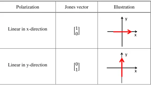
Table 1.1 and Table 1.2 show some general examples of Jones vector and Jones

matrices.

Polarization Jones vector Illustration

Linear in x-direction ₀₁ 01

Linear in y-direction ₀₀ 11

13 Linear at 45° 1 √20111 Right circular 1 √20 1−𝑖1 Left circular 1 √201𝑖1

Table 1-1 The reference between polarization and Jones vector.

Optical element Jones matirx

Neutral element _{01 0} 0 11 x-polarizer _{01 0} 0 01 y-polarizer _{00 0} 0 11 Quarter-wave retarder _{0 1} −𝑖 −𝑖 11 Half-wave retarder _{00 1} 1 01

Table 1-2 The reference between optical elements and Jones matrices.

1.3 Comparison of two diffraction theory

Through the discussion of scalar and vector diffraction theory, respectively, we

can find out some differences as following:

14

but scalar diffraction theory cannot.

2. The thickness of obstacle is assumed as zero in scalar diffraction theory, but it

must be taken into account in vector diffraction theory.

3. The scalar diffraction theory is only an approximation; therefore, that entails some

degree of error.

1.4 Motivation & Organization

Recently, the optical engineering is rapidly developed. More and more

parameters of light and material properties should be taken into consideration due to

the dimension of interested area is gradually reduced. Therefore, the scalar diffraction

theory is not suitable anymore; the vector diffraction theory is the only way to get

accurate solution. Polarization is also an important property of light in vector

diffraction theory; the different polarizations of light can elicit different effects in

material. Through the vector diffraction theory, we can observe the phenomenon of

interaction between light and material, and discuss the influence of polarization of

light in focus fields of light. Consequently, we hope we can obtain some useful

applications utilize the influence of polarization of light in this thesis.

This thesis will be partitioned into three major parts, first part of this thesis talks

about the effect of polarization in different numerical aperture in chapter 2, the

influence of polarization is more distinct when numerical aperture is bigger. It will be

demonstrated in later.

The second part is the first application of polarization which called extended

depth of focus; it is achieved through the synthesis of two orthogonal polarizations or

higher order of inhomogeneous polarization. It will discuss in chapter 3. The third

part is the second application of polarization which is utilized to excited

15

introduced in chapter 4.

16

Chapter 2

Polarization Beams

The mode of the electric field vibration is called “polarization”. According to

the beam with the same polarization at every point within the pupil plane or not, the

polarization beam can divide into homogeneous and inhomogeneous. In this chapter,

the focal field properties of two kinds of polarization will be shown in following.

2.1 Homogeneous and inhomogeneous polarization

Homogeneous polarization keep the identical polarization at every point within

the pupil plane; we can describe the field distribution by using the function dependent

on the ratio of electric field. If the beam only has the x-component of electric field, it

is called x-directional linear polarization. If the phase delay between x-component and

y-component is 90°, the polarization is called circular polarization.

As the standard operation process is not homogeneous among the pupil, it is

inhomogeneous polarization beam. The obvious difference can observe from Fig. 2-1

Fig. 2-1 (a) and (b) illustrates the homogeneous and in homogeneous beam, respectively.

17

which attracted much attention due to its symmetric feature. The general solution of

the wave equation for cylindrical vector beams includes two solutions: radially

polarized beam and azimuthally polarized beam. The orthogonal cylindrical vector

beams have the doughnut-shaped irradiance and good symmetry in r-direction or

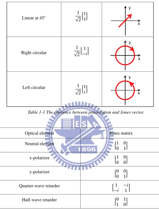
φ-direction. Due to the good symmetry, the radially polarized beam is p-polarization in omni-direction at the incident plane; likewise, the azimuthally polarized is

s-polarization, as shown in Fig. 2-2. Then the focused field distribution properties of

different polarization with different numerical aperture will be discussed in following.

Fig. 2-2 Intensity distribution of the cylindrical vector beams. (a) Radial (b) Azimuthal polarization.

2.2 Properties of polarized beam

In this section, the polarization states at the entrance pupil are linear, circular,

radial, and azimuthal, respectively. Examples of focal distribution with different

numerical aperture foci are shown.

2.2.1 Linear polarization

Considering an entrance pupil in which the polarization is x-direction linear

polarized and constant amplitude. The focused field distribution is circular symmetry

18

asymmetrical field which is larger along the direction of polarization due to the

electric field of z-components is no longer negligible in high numerical aperture, as

shown in Fig. 2-3. Therefore, the focused field is reduced which yields a broader

focus when numerical aperture is larger than 0.7. This is a direct result of the vector

effect.

Fig. 2-3 Intensity profile of linearly polarized focus as numerical aperture increases from 0.2 to 1.0, where the vectorial feature becomes more apparent with high-NA system.

19 2.2.2 Circular polarization

Now, considering an entrance pupil in which the polarization is right circular

polarized and constant amplitude. The focused field distribution is circular symmetry

no matter small or high numerical aperture, as shown in Fig. 2-4. Because of the

electric field of z-component has circular symmetry in the doughnut-shaped and

vanished on the optical axis. The x and y component are both asymmetrical but with

orthogonal axes, so the sum of each components is symmetrical.

Fig. 2-4 Intensity profile of circular polarized focus for increasing numerical aperture.

20 2.2.3 Radial polarization

For aforementioned polarization, their amplitude is constant, but for a radially

polarized pupil, amplitude forms a donut-shaped field because of the singularity in the

center. When numerical aperture is larger than 0.7, the optical field is transformed

from a doughnut-shaped to a flat-topped shape due to the depolarization effect starts

to govern the shape of the focused spot. Then the focused field of radially polarized

beams has a sharp intensity peak because of the strong depolarization effect which

caused the constructive interference of the z-component. Compared with linear

polarization and circular polarization, the smaller spot obtained from radial

polarization was under the conditions of numerical aperture larger than 0.9 and 0.95,

respectively [3], as shown in Fig. 2-5. But it was noted that superior illumination only exists in a high numerical aperture. On the other hand, because of the good polarized

symmetry in r-direction, the optical field still maintains circular symmetry for any

numerical aperture.

2.2.4 Azimuthal polarization

Azimuthal polarization is similar to radial polarization; the amplitude cannot be

constant and forms a donut-shaped field because of the singularity in the center and

due to the good polarized symmetry in φ-direction, the optical field also maintains

circular symmetry for any numerical aperture. The special focused feature of

azimuthal polarization is that yields a doughnut-shaped field even when numerical

aperture is larger than 0.7, as shown in Fig. 2-6. The reason of the special focused

field is that adjacent parts of this polarization are π-phase shifted with each other,

respectively. And another special focused feature is that electric field of z-component

is zero, therefore, the azimuthal polarization created an optical cage with the absence

21

Fig. 2-5 Intensity profile of radially polarized beams in different numerical aperture. When numerical aperture increased, the optical field is transformed from a doughnut-shaped to a flat-topped shape.

Fig. 2-6 Focused intensity profile of azimuthally polarized beams for high numerical aperture.

22

Fig. 2-7 Each component of focal fields in azimuthally polarized light, due to the destructive interference of depolarization effect, the electric field of z-component is zero.

2.3 Summary

The general solution with homogeneous and inhomogeneous polarization has been

discussed in aforementioned statement, respectively. Through the aforesaid discussion,

we can find out the homogeneous polarization is not suitable in high numerical

aperture system in terms of bigger focal spot size or changed shape of focused fields

which results from vector effect. For inhomogeneous polarization, due to the

depolarization effect in high numerical aperture, radial polarization could be focused

tighter beyond the diffract limits. It can further improve the resolution and be applied

to particle acceleration [4,5], particle-trapping [6], lithography [7], and material processing [8]. On the other hand, because of the specific phase distribution of azimuthal polarization, it can generate a sharper focal spot which smaller than the

focal spot of linear polarization when it propagates through a vortex 0-2π phase plate

[9]. As a consequence, inhomogeneous polarization becomes more important in many application of optics.

23

Chapter 3

Application 1 – Extended Depth of Focus

It is well known that imaging systems are sensitive to defocus error. Since

1950s, many groups made an attempt reduce the sensitivity of defocusing by

extending the depth of focus. In this chapter, we will introduce a novel polarization

coding technique without post signal processing.

3.1 History and Principle

From the view of wave optics, the defocusing aberration produces finite depth

of focus (DoF) because it introduces an additional quadratic phase in the pupil

function of the imaging system, resulting in a spatial low-pass filter effect. We will

demonstrate in following.

The optical transfer function (OTF) of a single-lens imaging system can be

written as a autocorrelation of the pupil function 𝑃(𝑥, 𝑦).

𝐻(𝑓𝑥, 𝑓𝑦) = ∬ 𝑃(𝑥 +𝜆𝑧_{2 , 𝑦 +}𝑖𝑓𝑥 𝜆𝑧_{2 )𝑃}𝑖𝑓𝑦 ∗_{(𝑥 −}𝜆𝑧𝑖𝑓𝑥 2 , 𝑦 − 𝜆𝑧_𝑖𝑓_𝑦 2 ) 𝑑𝑥 𝑑𝑦 ∞ −∞ ∬ |𝑃(𝑥, 𝑦)|∞ 2 −∞ 𝑑𝑥 𝑑𝑦 (3.1) Where 𝑓_𝑥, 𝑓_𝑦 are the spatial frequencies, 𝜆 is the wavelength of light, and 𝑧_𝑖 is the

distance from the lens to image plane. For a circular pupil, when defocusing

aberration is considering, the generalized pupil function will leads to the form

𝑃(𝑥, 𝑦) = |𝑃(𝑥, 𝑦)|𝑒𝑥𝑝,𝑖𝑘𝑊(𝑥, 𝑦)- (3.2) Where k = 2π/λ, and W(x, y) is the aberration function of defocusing, it has the

quadratic form

𝑊(𝑥, 𝑦) = 𝑊𝑚(𝑥 2_+𝑦2₎

𝑏2 (3.3)

24

the severity of the defocusing error, is given by

𝑊_𝑚= 𝑏2 2 ( 1 𝑧_𝑖 + 1 𝑧_𝑜− 1 𝑓) (3.4) Where zo is the distance from the object to the lens and f is the focal length of the lens.

When the imaging condition is not fulfilled (Wm is not zero), the OTF distribution is

narrower due to the quadratic phase factor arises. For the 1-D case Eq. (3.1) become

𝐻(𝑓𝑥, 𝑊𝑚) = ∫ 𝑃 (𝑥 +𝜆𝑧_{2 ) 𝑃}𝑖𝑓𝑥 ∗(𝑥 −𝜆𝑧𝑖𝑓𝑥 2 ) 𝑑𝑥 ∞ −∞ ∫ |𝑃(𝑥)|∞ 2 −∞ 𝑑𝑥 =∫ 𝑒𝑥𝑝 [ 𝑖𝑘𝑊_𝑚2𝜆𝑧_𝑖𝑓_𝑥𝑥 𝑏2 ] 𝑑𝑥 𝐴(𝑓𝑥) 2𝑏 (3.5) Where A(fx) is the 1-D overlap between two shifted pupil functions. Then Eq. (3.5)

gives the 1-D OTF

𝐻(𝑓_𝑥) = (1 −|𝑓𝑥| 2𝑓𝑐) 𝑠𝑖𝑛𝑐 [ 8𝑊𝑚𝜋 𝜆 ( 𝑓𝑥 2𝑓𝑐) (1 − 𝑓𝑥 2𝑓𝑐)] (3.6) Where

𝑓

_𝑐

=

𝑏

𝜆𝑧_𝑖 , when Wm is large value and the value of 𝑓𝑥 is not too large in comparison to 𝑓𝑐, that A(fx) can be approximated by A(0), where A(0) is the total area

of the pupil. Then the OTF can be approximated by

𝐻(𝑓_𝑥) ≈∫ 𝑒𝑥𝑝 [ 𝑖𝑘𝑊_𝑚2𝜆𝑧_𝑖𝑓_𝑥𝑥 𝑏2 ] 𝑑𝑥 𝐴(0) 2𝑏 =∫ 𝑒𝑥𝑝 [ 𝑖𝑘𝑊_𝑚2𝜆𝑧_𝑖𝑓_𝑥𝑥 𝑏2 ] 𝑑𝑥 𝑏 −𝑏 2𝑏 = 1 2𝑏∫ 𝑟𝑒𝑐𝑡 . 𝑥 2𝑏/ ∞ −∞ 𝑒𝑥𝑝 [𝑖𝑘𝑊𝑚2𝜆𝑧𝑖𝑓𝑥𝑥 𝑏2 ] 𝑑𝑥 = 𝑠𝑖𝑛𝑐(4𝑊𝑚𝜋𝑧𝑖𝑓𝑥 𝑏 ) (3.7) The expression of Eq. (3.7) demonstrates that defocusing aberration results a low-pass

filtering effect.

25

for overcome this limitation. In 1952, E. H. Linfoot and E. Wolf [10] computed the complete out-of-focus airy pattern for annular apertures and incidentally found out the

DoF was increased, then 1960, W. T. Welford [11] investigate the phenomenon in depth; this is the earliest and simplest method to reduce the defocusing aberration.

Due to the DoF is inverse proportion to pupil area, hence, through addition of binary

blocking mask in aperture plane, the DoF can be extend. The influence of additional

annular ring on total intensity field can be described mathematically

𝐼(𝑧) = 𝑎 4 𝜆2_𝑓2{ 𝑠𝑖𝑛 01_{2 𝑝(1 − 𝜀}2₎₁ 1 2 𝑝 } 2 , 𝑝 = 𝜋𝑎2𝑧⁄_𝜆𝑓2 (3.8)

Where a is radius of aperture, f is the distance from the exit pupil to the focus, and the

ε is obstruction ratio of radius as shown in Fig. 3-1.

Fig. 3-1 The configuration for annular aperture.

We can find out the total intensity field which does not change with different position

when ε is tending to unity. It means that DoF will extend to infinite, but unfortunately

when ε is larger, the side-lobe intensity of light fields and the obstructive area will

arise. Therefore, the system resolution and amount of light reaching the imaging plane

is lower.

26

system [12,13]. An extended DoF is obtained due to the overlap region of beams being diverted by refractive elements. As illustrated in in Fig. 3-2.

Fig. 3-2 The schematically concept of extending depth of focus by refractive optics.

Recently, because the computer develops vary rapidly; it brings another

technique which is called wave-front coding elements to extend depth of focus [14]. This method is not an all-optical approach due to that requires digital post-processing,

the idea involves that inserting a basically aberration which is much stronger than the

defocusing aberration such that by digital post-processing a sharp image can be

reconstructed.

One of the popular elements is the cubic phase element, in normalized

coordinates; the pupil function with cubic phase element is given by

𝑃(𝑥) = ,1⁄√2× 𝑒𝑥𝑝(𝑖𝛼𝑥3) 𝑓𝑜𝑟 |𝑥| ≤ 1

0 𝑜𝑡ℎ𝑒𝑟𝑤𝑖𝑠𝑒 (3.9) Where α is the coefficient which controls the phase deviation. Then the OTF related

to the pupil function can be approximated as

𝐻(𝑓_𝑥, 𝑊_𝑚) ≈ ( 𝜋 12|𝛼𝑓𝑥|) 1 2 ⁄ exp (𝑖𝛼𝑓𝑥 3 4 ) exp (𝑖 𝑘2_𝑊 𝑚2𝑓𝑥 3𝛼 ) , 𝑢 ≠ 0 (3.10)

27

When α is a larger value, the third part of the approximated of the OTF can be ignored,

therefore, the OTF will be independent of defocusing. Although this type of solution

can increased DoF plenty but rather one that requires digital post-processing, thus it

does not fit to ophthalmic. In addition to cubic phase mask, there are still some

another mask, i.e. free-form phase mask and exponential phase mask. [15,16] Then, a novel polarization coding technique will be introduced in following.

3.2 Combination of inhomogeneous beams

After realizing these methods which extending DoF utilize amplitude

manipulation or phase manipulation. In this section, we describe a novel

inhomogeneous polarization coding aperture to achieve extending DoF. In 2006,

Wanli Chi et al purposed this novel technique by combining two independent

orthogonal linear polarized lights [17]. As shown in Fig. 3-3, it has been demonstrated the effect which can extend DoF before. But in chapter 2, we already discuss the

properties with homogeneous and inhomogeneous light; the inhomogeneous polarized

light is superior to linear polarized light in terms of focus spot size or influence of

polarized direction in higher numerical aperture. Therefore, maybe we can not only

extend DoF but also increase the resolution by combing radial and azimuthal

polarized lights.

28

In the combination with radially and azimuthally polarized light, there are two

kinds of synthesis, as shown in Fig. 3-4. Manipulating the proportion between radially

and azimuthally polarized light, we can find out the best ratio to obtain maximum of

extending DoF. In Fig. 3-5 (a) to Fig. 3-5 (j), the radially polarized light is in outer

ring region and the central circular region is azimuthally polarized light. The opposite

arrangement of two polarized light is showed in Fig. 3-6 (a) to Fig. 3-6 (j). The

numerical number of system in here is 1.45.

Fig. 3-4 Two types of radial and azimuthal combination.

According to figures 3-4, we can find out the shape of light field is determined

by the polarization at outer ring region. The syntheses of two orthogonal polarizations

actually have the capability to extend depth of focus. The best combinative ratio of

radially polarized light to azimuthally polarized light is 3:7 when radially polarized

light is at the outer ring region. On the other hand, when azimuthally polarized light is

at the outer ring region, the ratio of radially polarized light to azimuthally polarized

light is 7:3; the results can obtain from Fig. 3-5(g) and Fig. 3-6 (g). In Fig. 3-7, we

discuss the full width at half maximum (FWHM) in z-axis of the two kind of best

combination, Fig. 3-7 (a) and (b) shows the slice of focus fields on z-axis, and FWHM

is 1.48 times and 1.7 times comparing combination and non-combination, respectively.

However, although the inhomogeneous polarization coded aperture can extend depth

of focus, but one of the aperture cannot obtain more better resolution than linear

29

Fig. 3-5 (a) to (j) peak intensity across different z-axis position when radially polarized light is in outer ring region.

30

Fig. 3-6 (a) to (j) peak intensity across different z-axis position when azimuthally polarized light is in outer ring region.

31

Fig. 3-7 The FWHM of (a) radially polarized light and (b) azimuthally polarized light focal fields.

Fig. 3-8 The intensity profile comparison between linear polarization coded aperture and in homogeneous coded aperture on x-y dimension.

good enough, as shown in Fig. 3-8.Therefore, we consider the depolarization effect of radially polarized light again, to obtain the good extended depth of focus due to

32 3.3 Higher-order radially polarized beam

In chapter 2, we already discussed the properties of fundamental mode of

radially polarized beam in terms of its strongly longitudinal component which results

by depolarization effect forms a tight focal spot in high numerical aperture system.

For this reason, recently, the higher-order radially polarized beam have been attracted

much attention due to it can effectively reduce the focal spot size by destructive

interference on horizontal components[18], it means that the higher-order radially polarized beam can produce a smaller focal spot size than fundamental mode in high

numerical aperture system. Therefore, in this section, we utilized the higher-order

radially polarized beam to achieve not only super-resolution but also extending DoF.

Since that very high longitudinal component has been achieved nearly flat top axial

distribution in focal volume.

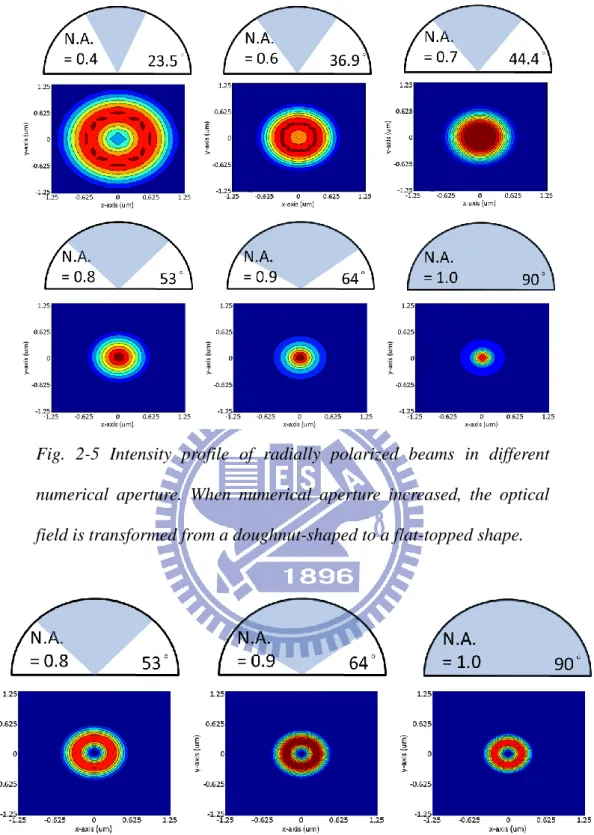
The order number of radially polarized beam depends on how many ring it has.

Single-ring-shaped beam is called fundamental mode radially polarized beam

(R-TEM01), and so on, double-ring-shaped beam is the first order of higher-order

radially polarized beam which called R-TEM11, as shown in Fig. 3-9. Here, we

compare the focus fields on z-axis between fundamental mode and two higher-order

modes.

Fig. 3-9 The fundamental mode (R-TEM01) and two higher-order

33

In Fig. 3-10, it shows the ability of extended DoF with higher-order radially

polarized beam, compare to fundamental modes (R-TEM01), the FWHM is 1.7 times

and 2.11 times in R-TEM11 and R-TEM21, respectively. Of cause, the better results can

be expected when the more higher-order to be chosen.

Fig. 3-10 The FWHM of focal fields of different order of radially polarized beam.

Although the higher-order radially polarized beam has many advantages, but it has a

vital constraint that the synthesis of higher-order beams is difficult to achieve. Up to

now, the strategy to generates higher-order radially polarized beam is nothing more

than through spatial light modulator (SLM) [19] or particular laser cavity design [20,21], but these synthesis methods are sensitivity to environment perturbation or precise manufacture. Therefore, the practical application of higher-order still has a

barrier to prevent the development.

3.4 Summary

In this chapter, we introduce two recipes of polarization coded to extend DoF;

one is the combination between radial polarization and azimuthal polarization, and the

34

cylindrical vector beam, we can achieve high spatial resolution as well as extended

35

Chapter 4

Application 2 – Chromatic Surface Plasmon Resonance

Recently, surface plasmon resonance (SPR) have been widely used to analyze

characteristics of material, providing quantitative and qualitative analyses due to its

unique character. In this chapter, the experimental setup for creating the chromatic

SPR and the optimized structure for objective-based configuration will be introduced

in the following.

4.1 History and Principle

The discovery of SPR begins at 1902, R. W. Wood observed a weird

phenomenon that didn’t obey the diffraction theorem of grating when the polarization

of light with electric field upright to the groove of metal grating [22]. He attempted to explain the phenomenon by oscillation with specific polarization of light and metal

grating structure. Until 1941, Fano purposed a new opinion about the interesting

phenomenon, he proposed a new electromagnetic wave along the surface when the

polarization of light with electric field upright to the groove of metal grating [23]. The electromagnetic wave is so-called SPR afterward. Then in 1950, R. H. Ritchie and R.

A. Ferrell et al purposed the theoretic model of SPR sequentially [24, 25], From then on, SPR elicited the interests of scientist, more attention invested in this study.

The SPR are collective oscillations of free electrons that can propagate between

the metal and dielectric surface. It is a kind of electromagnetic wave and confined

within the sub-wavelength of metal surface. Exactly as above said, the SPR are

electromagnetic wave, therefore, we can find the condition of existence of SPR from

Maxwell’s equation. In order to know the condition, we consider an interface between

36

The Maxwell’s equation at the surface between two media can be written as

𝛻 × 𝐻⃑⃑ = 𝜀𝑑𝐸⃑ 𝑑𝑡 (4.1a) 𝛻 × 𝐸⃑ = −𝑢𝑑𝐻⃑⃑ 𝑑𝑡 (4.1b) 𝛻 ∙ 𝜀𝐸⃑ = 0 (4.1c) 𝛻 ∙ 𝐻⃑⃑ = 0 (4.1d) Next considering s-polarization and p-polarization incident waves propagate

between two media as shown in Fig. 4-1, for s-polarization incident wave, the wave

function is

Fig. 4-1 (a) s-polarization (b) p-polarization waves propagate between two media.

z>0 𝐻⃑⃑ ₁ = (𝐻_𝑥1, 0, 𝐻_𝑧1) 𝑒𝑥𝑝(𝑘_𝑥1𝑥 + 𝑘_𝑧1𝑧 − 𝜔𝑡)𝑖 (4.2a) 𝐸⃑ ₁ = (0, 𝐸_𝑦1, 0) 𝑒𝑥𝑝(𝑘_𝑥1𝑥 + 𝑘_𝑧1𝑧 − 𝜔𝑡)𝑖 (4.2b) z<0 𝐻⃑⃑ ₂ = (𝐻_𝑥2, 0, 𝐻_𝑧2) 𝑒𝑥𝑝(𝑘𝑥2𝑥 − 𝑘𝑧2𝑧 − 𝜔𝑡)𝑖 (4.2c) 𝐸⃑ 2 = (0, 𝐸𝑦2, 0) 𝑒𝑥𝑝(𝑘𝑥2𝑥 − 𝑘𝑧2𝑧 − 𝜔𝑡)𝑖 (4.2d)

From Eq. (4.2a) to Eq. (4.2d), these equations must satisfy boundary condition, then

electric fields and magnetic fields at the surface are of the form (a) (b)

37

𝐸𝑦1 = 𝐸𝑦2 (4.3a)

𝑢₁𝐻_𝑧1 = 𝑢₂𝐻_𝑧2 (4.3b) 𝐻𝑥1 = 𝐻𝑥2 (4.3c)

𝑘_𝑥1 = 𝑘_𝑥2 (4.3d)

Substituting Eq. (4.2a) to Eq. (4.2d) into Eq. (4.1b) leads to

𝑘_𝑧1𝐸_𝑦1 = −𝑢₁𝜔𝐻_𝑥1 (4.4a) −𝑘𝑧2𝐸𝑦2 = −𝑢2𝜔𝐻𝑥2 (4.4b)

𝑘_𝑥1𝐸_𝑦1 = −𝑢₁𝜔𝐻_𝑧1 (4.4c) 𝑘𝑥2𝐸𝑦2 = −𝑢2𝜔𝐻𝑧2 (4.4d)

For nonmagnetic materials, 𝑢₁ ≈ 𝑢₂, according as Eq. (4.3a) to Eq. (4.3d), we can obtain a result of wave-vector

𝑘_𝑧1 = −𝑘_𝑧2 (4.5)

Comparing with dispersion relation

𝑘_𝑥12 _{+ 𝑘} 𝑧12 = 𝜀1. 𝜔 𝑐/ 2 (4.6a) 𝑘_𝑥22 _{+ 𝑘} 𝑧22 = 𝜀2. 𝜔 𝑐/ 2 (4.6b) We can know that Eq. (4.5) is contradiction if 𝜀₁ ≠ 𝜀₂ from Eq. (4.6). That because the s-polarization wave only has electron field along the surface, so there are no

electron accumulation. Hence, the SPR for s-polarization don’t exist at the surface, in

other words, the s-polarization incident wave cannot excite the SPR

For p-polarization incident wave, the wave function is

z>0

𝐻⃑⃑ 1 = (0, 𝐻𝑦1, 0) 𝑒𝑥𝑝(𝑘𝑥1𝑥 + 𝑘𝑧1𝑧 − 𝜔𝑡)𝑖 (4.7a)

38

z<0

𝐻⃑⃑ 2 = (0, 𝐻𝑦2, 0) 𝑒𝑥𝑝(𝑘𝑥2𝑥 − 𝑘𝑧2𝑧 − 𝜔𝑡)𝑖 (4.7c)

𝐸⃑ ₂ = (𝐸_𝑥2, 0, 𝐸_𝑧2) 𝑒𝑥𝑝(𝑘𝑥2𝑥 − 𝑘𝑧2𝑧 − 𝜔𝑡)𝑖 (4.7d)

From Eq. (4.7a) to Eq. (4.7d), these equations must satisfy boundary condition, then

electric fields and magnetic fields at the surface are of the form

𝐻_𝑦1 = 𝐻_𝑦2 (4.8a) 𝐸𝑥1 = 𝐸𝑥2 (4.8b)

𝜀₁𝐸_𝑧1 = 𝜀₂𝐸_𝑧2 (4.8c) 𝑘𝑥1 = 𝑘𝑥2 (4.8d)

Due to the symmetric of propagating wave at the interface, 𝐸_𝑧1 = −𝐸_𝑧2, then relation of permittivity between two media is

𝜀₁ = −𝜀₂ (4.9)

The significance of Eq. (4.9) indicated the SPR only exist and are excited on metal

which is negative index. Then Substituting Eq. (4.7a) to Eq. (4.7d) into Eq. (4.1a)

leads to 𝑘_𝑧1𝐻_𝑦1 = 𝜀₁𝜔𝐸_𝑥1 (4.10a) 𝑘𝑥1𝐻𝑦1 = −𝜀1𝜔𝐸𝑧1 (4.10b) 𝑘_𝑧2𝐻_𝑦2 = −𝜀₂𝜔𝐸_𝑥2 (4.10c) 𝑘𝑥2𝐻𝑦2 = 𝜀2𝜔𝐸𝑧2 (4.10d) 𝑘_𝑧1 𝜀₁ + 𝑘_𝑧2 𝜀₂ = 0 (4.10e) Finally, from Eq. (4.10e) and Eq. (4.8d) it leads to dispersion relation

𝑘𝑥1 = 𝑘𝑠𝑝𝑝(𝜔) = 𝜔 𝑐 √ 𝜀₁(𝜔)𝜀₂(𝜔) 𝜀1(𝜔) + 𝜀2(𝜔) (4.11a) 𝑘_𝑧𝑖 = √𝜀_𝑖𝑘₀2_{− 𝑘} 𝑥12 𝑖 = 1,2 (4.11b)

39

both media. Then permittivity of both media only can be

𝜀₁+ 𝜀₂ < 0 (4.12) 𝜀1∙ 𝜀2 < 0 (4.13)

The significance of Eq. (4.13) and Eq. (4.12) is similar to Eq. (4.9), which means that

not only either index of two media must be negative, but also the absolute value of

negative index exceeding that of the other. Most of the materials, especially noble

metals have large negative real part of dielectric constant. Therefore, the SPR can

exist at the interface between a noble metal and a dielectric when the polarization of

incident light is p-polarization.

After realized the condition of existence of SPR, we can find out only

p-polarization light can excite SPR on the interface between metal and dielectric, so

recently, radially polarized light has been wildly used to excite SPR due to the good

axial symmetric of p-polarization, and the merits of radially polarized light in terms of

a tighter focal spot already confirm in many investigations [26, 27]. But current technology does not allow for a simply frequency sweeping operation system for

radially polarized light. These major issues delay the progress on the development of

SPR and hinder further study on wavelength dependent material. Therefore, how to

simply create the white light radially polarized light and build up a polychromatic

radially polarized surface plasmon resonance (PC-RPSPR) sensor will be shown up in

following section.

4.2 Experimental Setup

The experimental setup of PC-RPSPR sensor can divide into two principal parts,

first part is synthesis of radially polarized white light utilized an approach of spatially

varying polarizer (SVP), as shown in Fig. 4-2 (a), and second part is the

40

We utilize an unpolarized white LED (model: Luxeon Star/O LXHL-NWE8) as a

light source which has advantages of low cost and is speckle free. A collimated

unpolarized light was converted to radially polarized light by the use of SVP. The

radially polarized white light then relays to the entrance pupil of the commercial

immersion objective lens (Olympus PlanApo-N 60x/1.45 Oil). Its corresponding half

divergence angle is 75.16°, well beyond the SPR resonant angle SP ~ 45o at

wavelength 0 = 610 nm. After passing through the objective, the white light focus on

the MIM structure, Non-coupled reflected light has been collected and guides

backward into two different optical paths via the same objective lens. One optical path

projected the reflected intensity distribution onto CCD image sensor from the back

focal plane of the objective lens. The other optical path records the spectra of reflected

beam via a spectrum analyzer. As shown in Fig. 4-2.

Fig. 4-2 Configuration of the PC-RPSPR sensor, where CL: collimated lens, SVP: spatial varying polarizer, RL: relay lens, BS: beam splitter, M: mirror, IL: image lens, MIM: metal-insulator-metal structure. The insets show (a) the photo of SVP, (b) the schematic diagram of MIM structure.

41

4.2.1 Synthesis of polychromatic radially polarized light

The SVP consists of eight pieces of linear polarizer and the transmission axis of

every sector aligned to individual principle radial direction, as shown in Fig. 4-3. The

SVP is used to convert unpolarized white light into radially polarized white light. In

microscopies, nano-optics, and spectroscopy, polychromatic radially polarized beams

can supply other perspectives. Based on past reported studies, the common recipe to

synthesis or generate radial polarization are designed for a specific working

wavelength and rely on the use of phase element, liquid crystal, interference

configuration [28, 29, 30, 31]. Those elements are wavelength dependent. This means that it cannot operate universally among different working wavelength in a fixed

design. However, only few numbers of devices can generate those kinds of light in

recently. The main systems are double conical reflector system which based on

geometrical optics [32] and fiber-based system [33]. Unfortunately, the former system crate a discontinuous ring beam shape, which decreases the resolution due to the

increment of side-lobe part in focal region and seems difficult to be apply for sensing;

the latter system need the procedure of precise optical alignment to couple incident

light into fiber. In other words, these systems are not simply and convenient. On the

contrary, proposed SVP is assembled by conventional polarizing element offering

wavelength independent properties for polarization conversion and simplify the

creative complexity of system. Also, it has a compact size with extremely low cost,

but this device exchanges those benefits for power consumption.

42 4.2.2 MIM Structure

The MIM structure (0 = 610 nm) is glass ( = 2.126) / 20 nm Au ( = -8.5 +

2.02i) / 400 nm SiO2 ( = 2.126) / 20 nm Au ( = -8.5 + 2.02i) sandwiched between

matching oil ( = 2.29) and a test sample (Air or Water), as shown in Fig. 4-2 (b). The function of the MIM structure is used to extend the sensing range of

refractive index for test sample up to about 1.42. According to the excitation

mechanism of SPR, the incidence angle, which provides sufficient wave-vectors to

agree phase matching conditions, is greater than the critical angle. The SPR angle is

wavelength dependent and is related to the dispersion relation of metal. Its resonance

angle shifts up when working wavelength decreased. Furthermore, generally the

refractive index of living cells are close to water (SPR, water ~ 77.4 o, 0 = 610 nm)

which beyond the sensing limit for objective lens with NA = 1.45 (max ~ 75.16°, 0 =

610 nm). Under this circumstance, the SPR dips are outside the observation windows

as the wavelength is smaller than 640 nm as shown in Fig. 4-4. Therefore, the MIM

structure is purposed,

As the beam focused on the MIM structure, not only cavity resonance (CR)

modes but also transformed surface plasmon resonance (T-SPR) modes which have

broader sensing range are generated. CR modes are insensitive to the change of the

refractive index of sample, but T-SPR mode is. The role of a MIM structure is to

transform generated cavity resonance (CR) modes into transformed surface plasmon

resonance (T-SPR) modes. The material and thickness of each layer determine the

resonance property of both modes. In order to maximum the depth of surface plasmon

resonant dips, we kept the symmetry property of MIM structure and set the overall

thickness of gold thin film as 40 nm, also, in order to confirm the effect of MIM

structure, we chose SiO2 as insulator which is identical to substrate. In our case, when