Electrophoretic Mobility of a Sphere in a Spherical Cavity
Eric Lee, Jhih-Wei Chu, and Jyh-Ping Hsu1
Department of Chemical Engineering, National Taiwan University, Taipei, Taiwan 10617, Republic of China Received January 7, 1998; accepted April 17, 1998
The electrophoretic behavior of a spherical particle in a spher-ical cavity is analyzed theoretspher-ically, taking the effect of double layer polarization into account. We show that for the case where the particle is positively charged and the cavity uncharged if the surface potential of particle is high, the variation of the mobility of the particle as a function of ka has a minimum, k and a being respectively the reciprocal Debye length and particle radius. This minimum does not appear if the effect of double layer polarization is neglected. The variation of the mobility as a function ofka has a minimum for a medium value of l (5 particle radius/cavity radius); it becomes negligible ifl is either small or large. In the case where the particle is uncharged and the cavity positively charged, if the surface potential is high, the variation of mobility as a function of ka has a maximum; if it is low, the mobility increases monotonically with ka. Here, the mobility is mainly determined by the drag force, rather than by the electric force, acting on the particle as in the case where the particle is positively charged and the cavity uncharged. If both the particle and the cavity are charged, the electrophoretic behavior of the particle can be deduced from the results of the above two cases. © 1998 Academic Press
Key Words: electrophoresis; mobility; double layer polarization;
spherical charged particle; boundary effect; spherical charged cavity.
1. INTRODUCTION
Knowledge about the surface potential of a charged entity is essential to various applications in practice. Typical example includes the adsorption of colloidal particles to a rigid surface and the coagulation behavior of a colloidal suspension (1). In practice, the surface potential is usually characterized by the zeta potential, the electrical potential at the shear plane of the electrical double layer near the charged entity which can be estimated on the basis of the electrophoretic mobility of the entity in an applied electrical field (1). The determination of the relation between the electrophoretic mobility and the zeta potential involves the solution of a set of differential equations, known as the electrokinetic equations (2). Due to its compli-cated nature, solving this set of equations analytically is almost impossible, in general, except for some limiting cases, in which
the electrokinetic equations can be simplified drastically. For an isolated sphere in an infinite fluid, for example, an analytical expression for the electrophoretic mobility as a function of zeta potential can be retrieved if the electrical potential is low, and the double layer is either very thin (3– 6) or very thick (7) relative to particle radius. The effect of double layer distortion due to the presence of the applied electric field on the electro-phoretic mobility was neglected in these studies. A numerical procedure is necessary if this effect is taken into account. The numerical solution for the electrokinetic equations was first provided by Wiersema et al. (8). O’Brien and White (9) sug-gested an effective numerical scheme for the resolution of the linearized electrokinetic equations. Their approach is valid for the case where the applied field is weak relative to that induced in the double layer around a particle. The electrophoretic behavior of a polyion in an infinite fluid was examined recently by Allison and Nambi (10); the governing equations were solved by a combined DIE/finite difference algorithm. The problem was also solved by using a boundary element method (11). They concluded that the accuracy of the spatial variation of electrical potential and ion density is crucial in the estima-tion of the electrophoretic mobility of a charged entity.
In practical applications, electrophoresis is almost always conducted in a finite domain, which implies that the boundary effect on the electrophoretic behavior of a particle may be significant. This effect makes the analysis much more compli-cated than that if the boundary is absent. A considerable amount of effort was made recently to examine the electro-phoresis in a bounded region (e.g., 12–15). Keh and Anderson (13) used the method of reflections to analyze the electro-phoretic motion of a particle normal to a large conductive plane, parallel to a large dielectric plane, along the axis of a long cylinder, and along the centerline between two large parallel plates. It was concluded that the results of Keh and Anderson are satisfactory forl , 0.7 (15–17), l being the ratio (linear size of particle/linear size of boundary). The electro-phoresis of a sphere through the center of a circular disk (18), that of an infinite insulating cylinder parallel to a planar wall (19), and that of an arbitrary prolate body of revolution towards an infinite conducting wall (20) were studied theoretically. All of these are based on the assumptions that the electrical double layer around a charged particle is infinitely thin relative to its linear size, and the electrical potential is low. In general, 1To whom correspondence should be addressed. E-mail: t8504009
@ccms.ntu.edu.tw.
65 0021-9797/98 $25.00
Copyright © 1998 by Academic Press All rights of reproduction in any form reserved.
obtaining an analytical expression for the mobility as a func-tion of zeta potential for a double layer of finite thickness is not an easy task. To simulate the electrophoretic behavior of a colloidal particle in a porous media, Zydney (14) considered the electrophoretic motion of a nonconductive spherical parti-cle at the center of a spherical cavity for the case of a finite double layer. This geometry was also adopted in the analysis of a concentrated suspension (21–25). It was concluded that the boundary effect is on the order ofl if the double layer is thick (14). This is different from that for a thin double layer where it is on the order of l3. Ennis and Anderson (26) used the method of reflections to investigate the electrophoresis of a spherical particle near a flat wall, in a slit, and in a cylindrical pore for the case of finite double layer thickness. It was assumed that the electrical potential is low, and the applied field is weak. The former implies that the Poisson–Boltzmann equation governing the variation of electrical potential can be approximated by a linear expression, which is readily solvable, and the latter implies that the effect of double layer distortion can be neglected. The analysis of Zydney (14) was extended recently by Lee et al. (27) to the case where a nonlinear Poisson–Boltzmann equation is considered. It was found that using a linearized Poisson–Boltzmann equation can lead to an
appreciable deviation in the electrophoretic mobility even the electrical potential is low.
The analysis of Lee et al. (27) neglected the effect of double layer distortion, a factor which may play a significant role in the determination of the electrophoretic behavior of a particle. This effect is taken into account in the present study.
2. THEORY
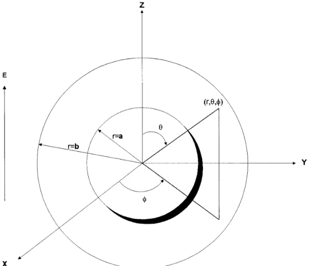
The system under consideration is illustrated in Fig. 1. A nonconducting, spherical particle of radius a is placed at the center of a spherical cavity of radius b, and a uniform electric field E in the z direction is applied. The spherical coordinates (r,u, f) are adopted in the following analysis. The electroki-netic equations include the ion conservation, the electrical potential, and the fluid dynamic equations. The conservation of ions leads to nj t 5 =h z
F
DjF
= h nj1 zjenj kT hf=G
1 njhvG
, [1]whereh= is the gradient operator, t the time, nj, Dj, and zjthe
number concentration, the diffusivity, and the valence of ion species j, respectively, e the elementary charge,f the electrical potential, and vh the fluid velocity. The electrical potential is governed by the Poisson equation:
=2f 5 2r « 5 2j
O
51M
zjenj
« , [2]
where« is the permittivity of the liquid phase and M the total number of ionic species.
The flow field is described by the Navier–Stokes equation under the creeping flow condition
=
h z vh 5 0, [3]
rf vt 5 h=h 2
v
h 2 =hp2r =hf @4# where p is the pressure, and rf and h the fluid density and viscosity, respectively. The last term on the right-hand side of Eq. [4] denotes the electrical body force. Here, we assume that the fluid is incompressible and has a constant viscosity. More-over, the motion of the particle is assumed to be slow so that the system is at a quasisteady state, and the terms that involve the time derivative in the governing equations can be ne-glected.
Suppose that the electrical potential,f, can be decomposed into the electrical potential that would exist in the absence of the applied electric field, f1, and that outside the particle arising from the applied electric field,f2, that is,f 5 f11f2. Following the same treatment as that employed by O’Brien and White (9), a perturbation function, gj, defined below is used to
describe the double layer polarization:
nj5 nj0exp
S
2zje~f11f21 gj!
kT
D
, [5]where k and T are, respectively, the Boltzmann constant and the absolute temperature, and nj0the bulk concentration of ion
species j. The pressure term in Eq. [4] can be eliminated by adopting the stream function representation (28):
i
h
fE4c 5 2
1
hsinu =h 3 ~r =h ~f11f2!! , [6]
where ihfis the unit vector in thef direction, c denotes the stream function, and the operator E4is defined as E45 E2E2:
E25 2 r21 sinu r2 u
S
1 sinu uD
. [6a]The r and theu components of the velocity vh, vr, and vu, can
be described in terms ofc by vr5 2 1 r2 sinu c u, [7a] vu5 1 r sinu c r . [7b]
Let us consider the case where both the particle and the cavity are nonconductive and each has a constant surface potential characterized by za and zb, respectively. Then, the
boundary conditions forf1are
f15zaat r5 a , [8a]
f15zbat r5 b . [8b]
The boundary conditions forf2are assumed as
f2
r 50 at r5 a , [9a]
f2
r 5 2Ezcosu at r 5 b . [9b]
We consider the case where the ion concentration remains at the equilibrium value on the cavity surface, and the surface of particle is ion-impenetrable. Therefore, we have
gj5 2f2at r5 b , [10a] 2zje kT gj r 5 1 Dj U at r5 a . [10b]
Under the applied electric field, the particle moves in the z direction with velocity U, the electrophoretic velocity. Suppose that the cavity remains fixed. These lead to the following boundary conditions for the Navier–Stokes equation:
vr5 U cosu, vu5 2U sinu at r 5 a , [11a] vr5 0, vu5 0 at r 5 b , [11b]
or in terms of the stream functionc as
c 5 212Ur2
sinu andcr 5 2Ur sin2u at r 5 a ,
[12a]
Since all the dependent variables are symmetric about the z axis, we have f1 u 5 f2 u 5 g1 u 5 g2 u 5 c 5 c u 50 atu 5 0 and atu 5 p . [13] Suppose that the liquid phase contains only one electrolyte (M5 2). Let z1and z2be, respectively, the valences of cation
and anion,a 5 2z2/z1. The electroneutrality in the bulk liquid
phase implies n205 (n10/a). The reciprocal Debye length, k, is
defined as k 5 @
O
j51 2 nj0~ezj! 2 /«kT #1/ 2 . [14]It can be shown that
n10z15 ~ka !2«kT ~1 1a !e2 a2 z1 . [15] Define UE5 («zk 2
/ha), which is the velocity of a particle predicted by the Smoluchowski’s theory when an electric field of strength (zk/a) is applied, wherezkiszaifzaÞ 0 and iszbifza5 0.
To simplify the mathematical manipulation, the governing equations are rewritten in a scaled form. In the discussion below, a symbol with an asterisk denotes a scaled quantity. Suppose that the applied electric field is weak so that the expressions for the distortion of double layer, the electric potential, and the flow field near a particle can be linearized. For example, the scaled number concentrations of ions, n*1and
n*2, can be approximated by
n*15 exp~2frf*1!@1 2fr~f*21 g*1!# , [16a]
n*25 exp~afrf*1!@1 1afr~f*21 g*2!# , @16b#
where g*j5 gj/zk, j5 1, 2, f*15f1/zk, f*25 f2/zk, and
fr5zkz1e /kT, wherezkisza, ifzaÞ 0, and is zbifza5 0.
The electrokinetic equations can be linearized by neglecting the terms that involve products of small quantities such as, g*1,
g*2, andf*2. For instance, the variation off*1becomes
=*2f* 15 2 1 ~1 1a! ~ka!2 fr @exp~2f rf1! 2 exp~afrf1!#. @17#
If the particle is charged and the cavity uncharged, the bound-ary conditions associated with Eq. [17] are
f*15 1 at r* 5 1, andf*15zb/zaat r*5
1
l , [17a]
where r*5 r /a, andl 5 a/b. If the particle is uncharged and the cavity charged, then the boundary conditions associated with Eq. [17] are
f*15 0 at r* 5 1, andf*15 1 at r* 5 1/l . [17b]
Similarly, the variation off*2is described by
=*2f* 22 ~ka !2 ~1 1a ! @exp~2frf*1! 1a exp~afrf*1!#f*2 5 ~ka ! 2
~1 1a ! @exp~2frf*1! g*11 exp~afrf*1!ag*2# . [18]
The associated boundary conditions are
f*2 r 50 at r*5 1 and f*2 r 5 2E*zcosu at r* 5 1 l , [18a]
where E*z5 Eza /za. The variation of g*j is described by
=*2 g*12fr= h *f*1z = h *g*15fr 2 Pe1h* z =v h *f*1, @19# =*2 g*21afr= h *f*1z = h *g*25fr 2 Pe2h* z =v h *f*1, @20# where Pej5 «(Z1e /kT) 2
/hDj, j 5 1, 2, is the electric Peclet
number of ion species j, and U*5U /UE. The associated
boundary conditions are
g*1
r* 5 2Pe1frU*cosu at r* 5 1, and g*15 2f*2at r*5 1/l, [20a] g*2 r* 5 Pe2fr a U*cosu at r* 5 1, g*25 2f*2at r*5 1 l. [20b]
The scaled Navier–Stokes equation is
E*4c* 5 ~ka ! 2 ~1 1a !
FS
g*1 u n*11 g*2 u an*2D
f*1 r*G
sinu . [21]The associated boundary conditions are
c* 5 212U*r*2 sinu at r* 5 1 , [21a] c* r* 5 2U*r* sin2u at r* 5 1 , [21b] c* 5c*r* 50 at r*51 l . [21c]
can be expressed as the product of a radial function and an angular function, and the solutions to Eqs. [17]–[21] subject to Eqs. [17a]–[21c] take the form
f*25 F2~r !cosu [22]
g*15 G1~r !cosu [23]
g*25 G2~r !cosu [24] c* 5 C ~r !sin2u
[25] On the basis of these expressions, the original problem be-comes one-dimensional. Equation [17] reduces to
Lf*15 2 1 ~1 1a ! ~ka !2 fr @exp~2f rf1! 2 exp~afrf1!# , [26] where the operator L is defined by
L; d 2 dr*21 2 r* d dr*2 2 r*2. [26a]
The associated boundary conditions are, if the particle is charged and cavity uncharged,
f*15 1 at r* 5 1 , [26b] f*15zb/zaat r*5
1
l. [26c]
If the particle is uncharged and cavity charged, the boundary conditions associated with Eq. [26] are
f*15 0 at r* 5 1 , [26d] f*15 1 at r* 5
1
l . [26e]
Similarly, Eqs. [18]–[21] reduce respectively to
F
L2 ~ka !2
11a @exp~2frf*1! 1a exp~afrf*1!#
G
F25 ~ka ! 2
11a @G1exp~2frf*1! 1aG2exp~afrF1!# , [27]
LG12fr df*1 dr* dG1 dr* 5 Pe1v*r df*1 dr* , [28] LG21afr df*1 dr* dG2 dr*5 Pe2v*r df*1 dr* , [29] and D4C 5 2~ka ! 2 11a
F
~n*1G11an*2G2! df*1 dr*G
, [30]where the operator D4is defined as D45 D2D2with
D25 d 2
dr*22
2
r*2. [30a]
The associated boundary conditions are: dF2 dr*5 0 at r* 5 1, [31a] dF2 dr*5 2E*zat r*5 1 l, [31b] dGj dr*5 2 Pej fr U* at r*5 1, j 5 1, 2, [31c] Gj5 2F2at r*5 1/l, j 5 1, 2, [31d] C 5 212U*r*2 anddC dr*5 2U*r* at r* 5 1, [31e] C 5dr*dC5 0 at r* 5l1. [31f] The mobility of a particle can be estimated on the fact that the sum of the external forces acting on it in the z direction which includes the electric force, FEz, and the hydrodynamic forces, FDz, vanishes at the steady state, that is,
FDz1 FEz5 0 . [32] The electric force can be calculated by
FEz5
EE
s
s ~2 =hf!d Ah, [33]
wheres is the surface charge density which is related to f1by Gauss’s divergence theorem. It can be shown that
FEz5 8 3p«za 2
S
r*df*1 dr* F2D
r*515 F*Ezp«za 2 , [34] where F*Ez5 8 3S
r* df*1 dr* F2D
r*51. [34a]In spherical coordinates, FDzcan be evaluated by (27) FDz5hp
E
0 pS
r4 sin3u r E2c r2 sin2uD
r5a du 2pE
0 pS
r2 sin2urf uD
r5a du . [35]On the basis of the linearized formulation adopted in the present study, this expression becomes, in terms of scaled quantities, FDz5 4 3p«za 2
S
r*4 r*S
D2C r*2DD
r*51 143p«za 2 ~ka ! 2 ~1 1aa !fr@r* 2@exp~2f rf*1! 2 exp~afrf*1!#F2#r*51. [36]For convenience, this expression is rewritten as
F*Dz5 F*Dfz1 F*Dez, [37] where F*Dz5 FDz p«za 2, [37a] F*Dfz5 4 3
S
r* 4 r*S
D2C r*2DD
r*51 , [37b] F*Dez5 4 3 ~ka !2 ~1 1aa !fr@r* 2@exp~2f rf*1! 2 exp~afrf*1!#F2#r*51. [37c]In Eq. [37], F*Dfzand F*Dezarise from, respectively, the viscous and the electric body forces exert on the particle. According to O’Brien and White (9), the problem of solving the linearized governing equations, Eqs. [26]–[31f], can be decomposed into two subproblems. The first one involves the solution of the problem that a particle moves at a uniform velocity U in the absence of the applied field. The boundary conditions associ-ated with this problem are
u*r5 U*cosu, and u*u5 2U*sinu at r* 5 1, [38a]
f*25 0 at r* 5
1
l. [38b]
In the second problem, the particle is fixed in the applied
electric field, and a no-slip condition is assumed at cavity surface. The boundary conditions are
u*r5 u*u5 0 at r* 5 1, [39a]
f*2
r* 5 2E*cosu at r* 5
1
l. [39b]
The force required to move the particle in the first problem, f1,
is proportional to U*, that is, f15 dU*. Similarly, the force
exerts on the particle in the second problem, f2, is proportional
to E*, that is, f25bE*. The fact that the sum of the external
forces acting on the particle vanishes leads to U*m5 2b/d, U*m
being the scaled mobility of the particle. Note that choosing the scaling factor UE for the electrophoretic velocity U has the
advantage of simplifying Eq. [21] so that the unknown terminal velocity of the particle will not present. The scaled mobility U*m thus obtained is the same as that of Zydney (14). The
mobility defined by O’Brian and White (9) can be expressed as 6pfrU*m.
The set of differential equations, Eqs. [26]–[30] are solved by a pseudospectral method (29) based on the Chebyshev polynomials. For the problem under consideration, this method is readily applicable and it has several desirable properties, such as a fast rate of convergence and the convergent proper-ties independent of the associated boundary conditions. Also, the mini–max property typically associated with the Cheby-shev polynomial is maintained. In our case, the computational domain is one-dimensional, and only the variations of the dependent variables in the r direction need to be determined. Here we assume that an unknown function f(r) can be ex-pressed in an Nth-order approximation:
fN~r ! 5
O
i50 Nf~ri!hi~r ! , [40]
where f(ri) is the value of f(r) at the ith collocation point. The
interpolation polynomial, hi(r), is a function of the collocation
points which are determined by mapping the computational domain of the radial variable r onto the interval of y, [21, 1], by
r5b2 a
2 y1
b1 a
2 . [41]
The (N 1 1) interpolation points in the interval [21, 1] are chosen to be the extrema of an Nth-order Chebyshev polyno-mial, TN(y), and
yj5 cos
S
pj
The corresponding interpolation polynomial hj(y) is hj~ y ! 5
F
~21! j11~1 2 y2!dTN~ y ! d yG
Y
@cjN 2~ y 2 y j!# , j5 0, 1, . . . , N , [43] where cjis defined by cj5H
2, j5 0, N . 1, 1# j # N 2 1 . [44] Differentiating Eq. [40] with respect to r yieldsdfN~r ! dr 5
O
i50 N dhi~r ! dr fN~ri! 5O
i50 NO
j50 N ~DN!ijfi~ xj! , [45]where (DN)ijdenotes the ijth element of the derivative matrix
which can be obtained by using the method proposed by Gottlieb (28). The governing equations, Eqs. [26]–[30], are rewritten in a discretized form. The discretized Eq. [26] is first solved by adopting a Newton–Raphson iteration scheme to obtainf*1first, and the rest of the discretized governing
equa-tions are then solved. Although the latter is a set of linear algebraic equations, the solution procedure still involves an iterative procedure since they are coupled. The independence of the solution on the number of grids is checked to ensure that the mesh used is fine enough, and the solution obtained is correct. Sixtyfive nodal points are used in the numerical pro-cedure. Double precision is used throughout the numerical computation.
3. DISCUSSION
Two cases are considered in the numerical simulations: (a) the particle is positively charged and the cavity uncharged, and (b) the particle is uncharged and the cavity positively charged.
3.1. Particle Positively Charged, Cavity Uncharged
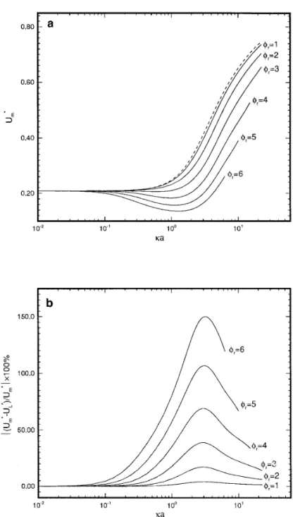
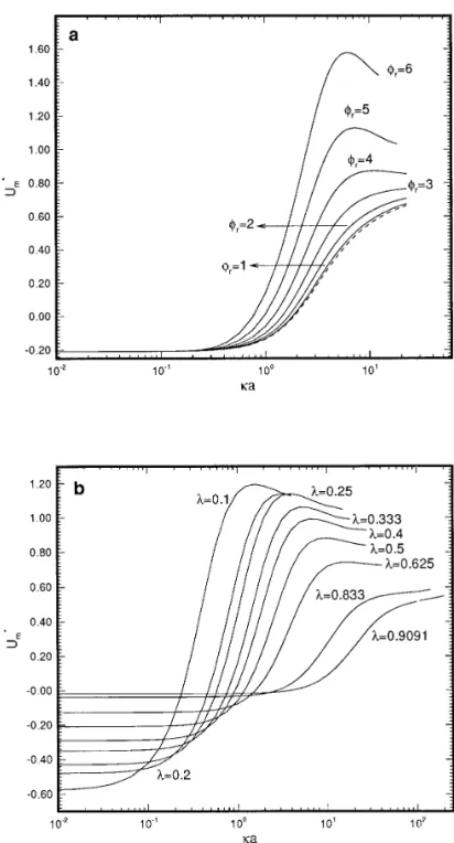
Figure 2a shows the variation of the scaled mobility of a particle, U*m, as a function of ka at various scaled surface
potential of particle,fr(5zaz1e /kT ), for the case where the
particle is positively charged and the cavity uncharged. The variation of the absolute percentage deviation of the mobility of a particle as a function ofka at various fris presented in
Fig. 2b. The percentage deviation is defined by |(U*m2U*L)/
U*m|3 100%, U*Lbeing the scaled mobility based on the model
where the linearized Poisson–Boltzmann equation is consid-ered and the double layer distortion neglected (14). Figure 2a and b reveal that, in general, the higher thefr, the greater the
deviation of the result based on the linearized Poisson–Boltz-mann equation from the present result, as expected. As can be
seen from Fig. 2b, this deviation vanishes, however, ifka is either very large or very small. In other words, the result of Zydney (14) can be recovered as the limiting case of the present study. Figure 2a shows that for a low to mediumfr,
U*mincreases with ka. If fris high, the variation of U*mas a
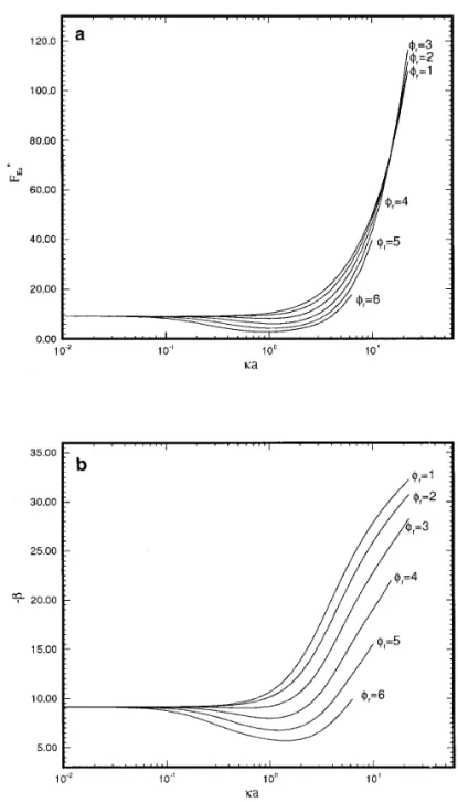
function of ka has a minimum. This was also observed by Wiersema (8) and O’Brien (9) for the electrophoresis of a spherical particle in an infinite fluid. The rationale behind this can be elaborated as following. According to the theoretical deviation, the mobility of a particle can be expressed as the
FIG. 2. (a) Variation of the scaled mobility of a particle, U*m, as a function ofka at various scaled surface potential of particle, fr, for the case where the
particle is positively charged and the cavity is uncharged. The dashed line represents the result based on the linearized Poisson–Boltzmann equation. (b) Variation of the absolute percentage deviation of the mobility of a particle as a function ofka at various fr. U*Lis the result based on (14). Key:l 5 0.5, Pe15 Pe25 0.1, anda 5 1.
ratio2b/d. The numerator is the force exerts on the particle, which is fixed at the center of the cavity, per unit electric field, and the denominator that per unit velocity of particle in the absence of electric field. These forces are determined by the sum of FEz and FDz. Therefore, both d and b are related to double layer distortion and are functions ofF2, G1, and G2, as
suggested by Eqs. [34], [36], and [37]. Due to the linearization of governing equations, however,d and b are independent of E* and U*. According to Eq. [34], F*Ez is determined by the product (df*1/dr*)F2. The value of (df*1/dr*), or the surface
charge density, increases withka. However, since the electric field in the double layer increases withka also, the effect of the applied electric field is lessened, andF2decreases. The higher thefr, the more significant this effect is. Therefore, the
vari-ations of F*Ez and the resultant2b as a function of ka has a minimum at a higherfr. This can be justified by the fact that
the qualitative behaviors of F*Ezand2b follow the same trend, as shown in Fig. 3a and b. The minimum does not appear if the effect of double layer distortion is neglected. Note that U*mis
independent offrifka is fixed in Zydney’s result (14).
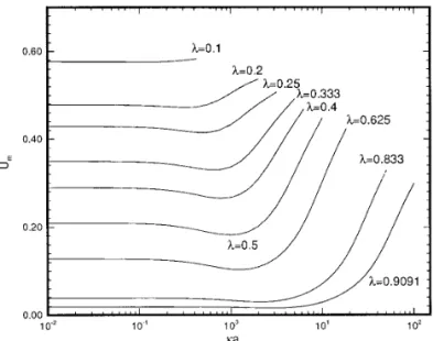
Figure 4 shows the variation of the scaled mobility U*mas a
function of ka at various l (5 radius of particle/radius of cavity). As can be seen from this figure, the variation of U*mhas
a minimum ifl has a medium value; it becomes inappreciable ifl is small or large. According to Zydney (14), if ka is small, the effect of the spherical boundary on the mobility of a spherical particle is on the orderl, and on the order l3, ifka is large. This implies that the result for an isolated particle can be deduced from the present system at a small l. The curve corresponding tol 5 0.1 in Fig. 4, for example, is approximate to the variation of the scaled electrophoretic mobility of an isolated spherical particle as a function ofka.
The variation offrc, the scaled surface potential of particle
at which the mobility has the minimum, as a function ofl is presented in Fig. 5a, and the variation ofkac, the value ofka
at which the mobility has the minimum, as a function offrat
variousl shown in Fig. 5b. If l is small, the distance between the particle and the cavity is large. As a result, the decrease in
F2due to the electric field induced in the double layer around the particle is lessened, and, therefore, it is relatively difficult for U*mto have a minimum. On the other hand, ifl is large, the
motion of the particle is confined in a limited space, and it is also difficult for U*m to have a minimum. This is why the
variation offrcas a function ofl has a minimum, as shown in
Fig. 5a. Figure 5b suggests that, ifl is large, the variation of
kacas a function of fr may have a maximum. Whether this
maximum appears depends largely on the relative rate of variations of (df*1/dr*) andF2as a function ofka.
3.2. Particle Uncharged, Cavity Positively Charged
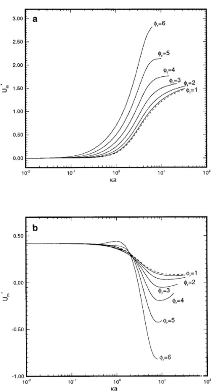
Figure 6(a) shows the variation of the scaled mobility of a particle, U*m, as a function of ka at various scaled surface
potential of cavity, fr (5zbz1e /kT), and that at various l
shown in Fig. 6b for the case where the particle is uncharged and the cavity positively charged. For comparison, the result based on the linearized Poisson–Boltzmann equation and ne-glecting the effect of double layer distortion (14) is also pre-sented in Fig. 6a. According to Zydney (14), if ka 3 0, negative charges will be induced on particle surface due to the presence of the positively charged cavity. Therefore, the par-ticle will move in the 2z direction, that is, the mobility is negative. As ka increases, the double layer near the cavity surface becomes thinner, and the amount of induced negative charges on particle surface decreases. The concentrated anions in the double layer near cavity surface leads to an
electroos-FIG. 3. (a) Variation of FEzas a function ofka at various scaled surface
potential of particle,fr, for the case where the particle is positively charged
and the cavity is uncharged. (b) Variation of2b as a function of ka at various
fr. U*mand U*Lare, respectively, the scaled mobility based on the present study and that on (14). Key: same as Fig. 2.
motic flow under the influence of the applied electric field. A clockwise vortex flow will appear, and the particle experiences a drag force in the z direction. Therefore, the mobility of the particle may become positive aska increases, and approaches the limiting result as that reported by Zydney (14) aska 3 `. In our case, the double layer distortion makes the problem more complex. As revealed by Fig. 6a, for a higher fr, the
variation of U*mas a function ofka has a maximum, and if fr
is low, U*mincreases monotonically with ka. Figure 6b
sug-gests that for a small to medium l the variation of U*m as a
function of ka has a maximum. Due to the limitation of the available space for particle movement, the maximum mobility is relatively difficult to achieve ifl is large.
The variations of F*Dfz and F*Ez as a function of ka at various scaled surface potential of cavity fr are illustrated
in Fig. 7. In contrast to the case where the particle is charged and the cavity uncharged, the behavior of the mobility is mainly determined by one of the scaled components of the drag force F*Dz, F*Dfz, defined in [37b], rather than by the electric force F*Ez. As suggested by Fig. 7a, F*Dfz3 0 as ka
3 0. As ka increases, the strength of the electroosmosic
flow increases, so does F*Dfz. However, the variation of F*Dfz as a function ofka has a maximum if fr is high. Since the
strength of the electroosmotic flow is determined by (df*1/
dr*) and Gj, j 5 1, 2, as suggested by Eq. [30], and Gj is
related to F2, as suggested by Eq. [31d], the existence of this maximum is a function of F2, which is due to the presence of the applied electric field. As can be seen from Fig. 7b, iffr is high, the variation of F*Ezas a function ka has a minimum. This is because that (df*1/dr*)r*51decreases
with an increase inka, and the variation of F2as a function ofka has a minimum (note F2is negative). In other words, the influence due to the applied electric field, measured by
F2, has a minimum as ka varies. This has an indirect
influence on the flow field. The strength of the electroos-mosic flow is increased, and the mobility of a particle has a maximum. This phenomenon is not observed in the case where the particle is charged and the cavity is uncharged.
The variation offrc, the scaled surface potential of cavity at
which the mobility has the extreme value, as a function ofl is shown in Fig. 8a. This figure reveals thatfrcincreases
mono-tonically withl. This is different from the result for the case where the particle is charged and the cavity uncharged. The variation ofkac, the value ofka at which the mobility has an
extreme value, as a function offrat variousl is illustrated in
FIG. 4. Variation of the scaled mobility U*mas a function ofka at various
l (5 radius of particle/radius of cavity) for the case where fr5 4. The particle
is positively charged, and the cavity is uncharged. Key: same as Fig. 2.
FIG. 5. (a) Variation of frc, the scaled surface potential of particle at
which the mobility has the minimum, as a function ofl. (b) Variation of kac,
the value ofka at which the mobility has the minimum, as a function of frat
various l. The particle is positively charged, and the cavity is uncharged. Parameters used are Pe15 Pe25 0.1 anda 5 1.
Fig. 8b. As can be seen from this figure,kacdecreases
mono-tonically with the increase infr.
3.3. Both Particle and Cavity Are Charged
If both the particle and the cavity are charged, the elec-trophoretic behavior of a particle can be deduced from the results of the above two cases. Figure 9a and b, for example, show respectively the variations of the scaled mobility of a particle, U*m, as a function of ka at various scaled surface
potential of particle, fr, when both the particle and the
cavity are positively charged and when the particle is pos-itively charged and the cavity negatively charged. The re-sults based on the linearized Poisson–Boltzmann equation are also shown in these figures. A comparison between Figs. 2a and 9a reveals that the U*m for the case where both the
particle and the cavity are positively charged is greater than that for the case where the particle is positively charged and the cavity uncharged. This is because that the electroosmotic flow induced by the cavity is in the same direction as that of
FIG. 7. (a) Variation of F*Dfzas a function ofka at various scaled surface potential of cavity,fr. (b) Variation of F*Ezas a function ofka at various fr.
The particle is uncharged, and the cavity is positively charged. Key: same as Fig. 6 exceptl 5 0.5.
FIG. 6. (a) Variation of the scaled mobility of a particle, U*m, as a function ofka at various scaled surface potential of cavity, fr(5zbz1e /kT), for the case l 5 0.5. The particle is uncharged, and the cavity is positively charged. The
dashed line denotes the result based on (14). (b) Variation of U*mas a function ofka at various l. Key: Pe15 Pe25 0.1 anda 5 1.
the electric force. Also, due to the presence of the electroos-motic flow, the minimum of the variation of U*m as a
function of ka at a high fr in Fig. 2a vanishes, as can be
seen in Fig. 9a. Similar to the case of Fig. 2a, the higher the
fr, the greater the deviation of the result based on the
linearized Poisson–Boltzmann equation from the present result. In contrast to Fig. 2a, however, the deviation is positive. Figure 9b suggests that, if the particle is positively charged and the cavity negatively charged, the variation of U*mas a function ofka has a minimum for a low fr, and a
maximum and a minimum for a high fr. If fr is low, the
positive charge induced on particle surface due to the pres-ence of the negatively charged cavity is limited. In this case, U*m decreases first with the increase in ka for a small to
mediumka, and then increases with a further increase in ka due to the influence of the electroosmotic flow. Iffris high,
the positive charge induced on particle surface is apprecia-ble, and U*mincreases with the increase inka for a small to
mediumka. As ka becomes large, the electroosmotic flow,
FIG. 9. Variation of the scaled mobility of a particle, U*m, as a function of
ka at various scaled surface potential of particle, fr. (a) Both the particle and
the cavity are positively charged,f*1(r*5 1) 5f*1(r*5 1/l) 5 1; (b) the particle is positively charged and the cavity is negatively charged,f*1(r*5 1)
5 1,f*1(r*5 1/l) 5 21. The dashed line represents the result based on the linearized Poisson–Boltzmann equation. Key: same as Fig. 2.
FIG. 8. (a) Variation offrc, the scaled surface potential of cavity at which
the mobility has the maximum, as a function ofl. (b) Variation of kac, the
value ofka at which the mobility has the maximum, as a function of frcat
variousl. The particle is uncharged, and the cavity positively charged. Key: same as Fig. 6.
which has an opposite direction to the electric force, be-comes dominant, U*m decreases, and, therefore, it has a
maximum.
It should be pointed out that the numerical scheme adopted in the present study is inefficient ifka is greater than about 10. This is because when ka is large, the double layer near a charged surface is thin, and the spatial variation of the electri-cal potential inside becomes very steep. In this case, solving Eq. [2] numerically is not recommended, and a semianalytical approach such as perturbation method is suggested.
Although the model system considered here is an imaginary one, it simulates some important cases in practice, such as a particle in a porous medium, and, therefore, it provides valu-able information about the effect of a rigid boundary on the electrophoretic behavior of a particle. As pointed out by Zyd-ney (14), however, that since the electroosmotic flow observed in the present system is due to the presence of a closed boundary, the behavior of a particle predicted here may be different from that based on an open system, such as a particle in a cylindrical pore, or a particle near a planar surface.
ACKNOWLEDGMENT
This work is supported by the National Science Council of the Republic of China.
REFERENCES
1. Hunter, R. J., in “Zeta Potential in Colloid Science.” Academic Press, New York, 1981.
2. Hunter, R. J., in “Foundations of Colloid Science,” Vols. I and II. Clar-endon Press, Oxford, 1989.
3. Smoluchowski, M., Z. Phys. Chem. 92, 129 (1918).
4. Dukhin, S. S., and Derjaguin, B. V., in “Surface and Colloid Science,” Vol. 7. Wiley, New York, 1974.
5. O’Brien, R. W., and Hunter, R. J., Can. J. Chem. 59, 1878 (1981). 6. O’Brien, R. W., J. Colloid Interface Sci. 92, 204 (1983). 7. Hu¨ckel, E., Phys. Z. 25, 204 (1924).
8. Wiersema, P. H., Loeb, A. L., and Overbeek, J. Th. G., J. Colloid Interface Sci. 22, 78 (1966).
9. O’Brien, R. W., and White, L. R., J. Chem. Soc., Faraday Trans. II 74, 1607 (1978).
10. Allison, S. A., and Nambi, P., Macromolecules 27, 1413 (1994). 11. Allison, S. A., Macromolecules 29, 7391 (1996).
12. Jorgenson, J. W., Anal. Chem. 58, 743A (1986).
13. Keh, H. J., and Anderson, J. L., J. Fluid Mech. 153, 417 (1985). 14. Zydney, A. L., J. Colloid Interface Sci. 169, 476 (1995). 15. Keh, H. J., and Chiou, J. Y., AIChE J. 42, 1397 (1996).
16. Morrison, F. A., and Stuhel, J. J., J. Colloid Interface Sci. 33, 88 (1970).
17. Keh, H. J., and Chen, S. B., J. Fluid Mech. 194, 377 (1988). 18. Keh, H. J., and Lien, L. C., J. Fluid Mech. 224, 305 (1991).
19. Keh, H. J., Horng, K. D., and Kuo, J., J. Fluid Mech. 231, 211 (1991). 20. Feng, J. J., and Wu, W. I., J. Fluid Mech. 264, 41 (1994).
21. Levine, S., and Neale, G. H., J. Colloid Interface Sci. 47, 520 (1974). 22. Kozak, M. W., and Davis, E. J., J. Colloid Interface Sci. 112, 403
(1986).
23. Kozak, M. W., and Davis, E. J., J. Colloid Interface Sci. 127, 497 (1989). 24. Kozak, M. W., and Davis, E. J., J. Colloid Interface Sci. 129, 166 (1989). 25. Ohshima, H., J. Colloid Interface Sci. 188, 481 (1997).
26. Ennis, J., and Anderson, J. L., J. Colloid Interface Sci. 185, 497 (1997). 27. Lee, E., Chu, J. W., and Hsu, J. P., J. Colloid Interface Sci. 196, 316
(1997).
28. Happel, J., and Brenner, H., in “Low-Reynolds Number Hydrodynamics.” Martinus Nijhoff, Boston, MA, 1983.
29. Canuto, C., Hussaini, M. Y., Quarteroni, A., and Zang, T. A., in “Spectral Methods in Fluid Dynamics.” Springer-Verlag, New York, 1986.