A lattice framework for analyzing context-free languages with applications in parser simplification and data-flow analysis

A Lattice Framework for Analyzing Context-Free

Languages with Applications in Parser Simplification and

Data-Flow Analysis

Department of Computer and Information Science National Chiao Tung University

Hsinchu, Taiwan 300, R.O.C.

We propose a lattice framework for analyzing free grammars and context-free languages. This framework is motivated by a technique for simplifying parsers with information derived from the associated scanners. We define the lattice framework and demonstrate it using additional applications, including data-flow analysis. Soundness and other properties of the lattice framework are also discussed.

Keywords: compiler, context-free grammar, finite-state machine, lattice, Mealy machine,

parser, regular expression, scanner

1. INTRODUCTION

In this paper, we first propose a technique for simplifying parsers using information derived from scanners (Sections 2 through 4). We then describe a lattice framework under-lying the technique (Sections 5 and 6). The lattice framework can be used to analyze many properties of context-free grammars and context-free languages. We demonstrate the lat-tice framework using several additional examples, including a data-flow analysis problem. Soundness and other properties of the lattice framework are also proved.

The front-end of a traditional compiler consists of a scanner and a parser. The scan-ner and the parser form a producer/consumer relationship: the scanscan-ner produces a stream of tokens from an input character stream while the parser consumes the tokens. Since the parser has no control over what the scanner will produce, the parser usually assumes that its input is an arbitrary sequence of tokens. However, in a previous paper [1], we proposed that the scanner should be described by a Mealy machine [2] (rather than a Moore machine), in which tokens produced by a scanner are associated with state transitions, rather than states. A Mealy-machine description implies that what the scanner produces is not an arbitrary sequence of tokens; rather, the sequence of tokens produced by the scanner is defined by a regular expression. When the input to the parser is defined by a regular expression, it is possible to simplify the parser (by means of removing states, transitions, and production rules) using information derived from the regular expression.

Received April 29, 1997; accepted September 15, 1997. Communicated by Jang-Ping Sheu.

This work was supported in part by the National Science Council, Taiwan, R.O.C., under grant NSC 85-2213-E-009-051.

We first describe a new, algebraic technique to extend the transition function of the

characteristic output machine of the scanner (to be defined in Section 2). The extension is

encoded in a ⊕ operator. The ⊕ operator is used to set up equations on sets of states. These equations are solved by an iteration algorithm. Based on the solution of the equations, we can identify useless transitions and unreachable states of the finite-state machine underly-ing an LR parser. It is also possible to eliminate production rules from the grammar in certain cases. In this paper, we demonstrate the technique on an LR(0) machine. However, it is straightforward to apply the technique to other LR(k) machines.

The simplification technique is actually a special case of a general lattice framework underlying context-free languages. A context-free language is defined by a context-free grammar, which contains terminals, nonterminals, and production rules. We may adopt a different view of a context-free grammar: The terminals and nonterminals denote sets of strings; the production rules are equations specifying relationships among these sets. The equations can be solved for the sets denoted by the nonterminals. The context-free lan-guage is the set denoted by the start symbol of the grammar. For instance, let A → UVW |

XYZ be the set of all the A-productions (where the A-productions are the productions whose

left-hand-sides are the nonterminal A) in a grammar. These A-productions can be viewed as the equation A = (UVW) ∪ (XYZ). From this viewpoint, a context-free language is defined, not in isolation, but by means of relationships among closely related sets (i.e., those sets denoted by terminals and nonterminals).

We might be interested in some properties of a context-free language. For instance, we might want to know whether all the sentences of a context-free language have even lengths. Since a context-free language is a set of sentences and a sentence is the concatena-tion of symbols, a property of a context-free language is the aggregate of the properties of individual sentences, and the properties of individual sentences are the aggregates of the properties of individual symbols. Note that the aggregation corresponds closely to the production rules. Hence, the production rules may be viewed as equations defining rela-tionships among properties of terminals and nonterminals. For instance, the above set of A-productions can be viewed as the equation fA=(fU ⊗ fV⊗ fW)♦(fX ⊗ fY⊗ fZ), where fA denotes a property of (the set represented by) the nonterminal A, and ⊗ and♦are the aggre-gation operations corresponding to the concatenation and the | operators in the production rules, respectively. Thus, a property of a context-free language is defined, not in isolation, but by means of relationships among properties of closely related languages. (Note that each terminal or nonterminal denotes a context-free language.)

We can solve the equations if the domain-of-interest is a finite lattice in which the aggregation operator♦is theB(or A) operation. Note thatB(orA, respectively) acts “accumulatively”; that is, if x ≤ y, then x By = y (or x Ay = x, respectively). If ⊗ satisfies certain desirable properties, we can solve the equations by gradually accumulating the re-sults from the least (or greatest, respectively) elements of the lattice. Since the lattice is finite, the accumulation process is guaranteed to terminate. It is found in Sections 2 through 4 that the simplification technique makes use of two such lattice frameworks. We also find that many other interesting problems can be solved using a lattice framework. We charac-terize the lattice framework and prove several fundamental properties of the framework.

The remainder of this paper is organized as follows. Section 2 reviews the Mealy-machine description of a scanner and defines the characteristic output Mealy-machine of the scanner. Section 3 presents an algebraic technique to extend the characteristic output machine. We

will use the results to simplify parsers, which are described in Section 4. In Section 5, we propose a lattice framework for analyzing context-free grammars and context-free languages. Several additional examples are used to demonstrate the framework. In Section 6, we show that when a lattice framework is used to analyze context-free languages, the results of analysis are independent of the particular context-free grammars used to describe the con-text-free languages. Properties of the language-analysis schemes are also discussed. In Section 7, we briefly discuss the language-analysis schemes based on an infinite lattice. The last section concludes this paper and discusses related work.

2. COMPUTING THE CHARACTERISTIC OUTPUT MACHINE OF A SCANNER

A scanner is formally specified by a set of regular expressions defining various kinds of tokens. Ambiguities encountered during scanning are resolved by the longest match

rule. For instance, the string “123456” is considered an integer of six digits rather than six

integers of one digit each. The longest match rule forces the scanner to look ahead a few characters in deciding the end of a token. If the scanner looks ahead only a finite number of characters, its look-ahead behavior can be integrated into the finite-state machine by asso-ciating a scanner’s output with state transitions. That is, a Mealy machine can accommo-date the finite look-ahead behavior quite well and, hence, is a better model of scanners [1]. The process of creating the Mealy machine of a scanner is described in detail in [1].

The output of a scanner, which is a Mealy machine, can also be described by a finite-state machine. The characteristic output machine (COM) of a Mealy machine is obtained by ignoring the input components on transitions in the Mealy machine. If there is no output token associated with a transition, that transition will be an ε-transition. The resulting COM is usually deterministic. A deterministic COM can be obtained from the non-deterministic COM by means of the subset construction technique[3].

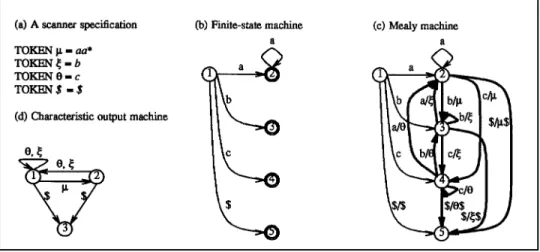
Example: Consider the scanner specification in Fig. 1(a), which defines four kinds of tokens.

The $ is the end-of-file character, which is also the end-of-file token. Fig. 1(b) is the finite-state machine of the scanner. The double-circles denote accepting finite-states. State 1 is the initial state. Fig. 1(c) is the Mealy machine of the scanner, in which output is associated with transitions rather than states. The bold-face edges are the augmented edges. The notation c/µ on an edge means that for input character c, the Mealy machine will produce an output token µ. Note that Fig. 1(c) is actually a generalized Mealy machine in the sense

that a sequence of zero or more tokens may be associated with a transition. When the input components on the edges of Fig. 1(c) are ignored, a nondeterministic COM is obtained. This nondeterministic COM can be transformed into a deterministic one using standard techniques. The resulting characteristic output machine is shown in Fig. 1(d). Note that the characteristic output machine does not accept a trivial regular expression; in particular, it cannot accept two consecutive µ’s. Hence, the scanner is singular (defined below).

Definition: A scanner is non-singular if it can produce an arbitrary stream of tokens ending

The stream of tokens produced by a non-singular scanner is the trivial regular ex-pression (µ | ξ | θ | ...)*$, where µ, ξ, θ,.... are the tokens, and $ is the end-of-file mark. On the other hand, the stream of tokens produced by a singular scanner is described by a non-trivial regular expression. Intuitively, a singular scanner provides additional information about its output. Most scanners are singular. (Consider that most scanners cannot produce two consecutive integers without an intervening space.) Though practical programming languages avoid singularity by allowing blanks and comments to be inserted between to-kens in the source programs, some programming languages do not allow such arbitrary white spaces. For instance, some VLSI description languages are translated into intermedi-ate languages for further processing. Since the intermediintermedi-ate languages are not intended for humans to read or write, they can forbid blanks and comments. The technique proposed in the paper will be useful in these intermediate languages.

A parser usually assumes that it takes input from a non-singular scanner. If it is known that the parser takes input from a singular scanner, additional information can be obtained from the characteristic output machine of the scanner. The information can be used to simplify parsers. We will discuss this technique in the following two sections.

3. EXTENDING THE CHARACTERISTIC OUTPUT MACHINES

The interface between a scanner and a parser is the stream of tokens. The stream of tokens must be accepted by the COM of the scanner and must orm to the context-free grammar of the parser. Therefore, we seek a relationship between a finite-state machine and a context-free grammar.

Let M be a finite-state machine and G be a context-free grammar. We define an operator ⊕ that takes two arguments: a set of states (of M) and a string of terminals and nonterminals (of G). The result of ⊕ is a set of states (of M). The notation Q ⊕α = Q′

means that, starting from a state of Q, M will reach a state of Q′ on an input string that is

derivable from the string α (according to the production rules of G). ⊕ may be viewed as an extension of the transition function of the COM of a scanner to the nonterminals of the context-free grammar of a parser. The operator ⊕ is defined by the following four axioms: (1) {q} ⊕ a = {q′ | M moves from state q to state q′ on input a, where a is a terminal of

G }.

(2) {q} ⊕ A = {q′ | M moves from state q to state q′ on a string of terminals α, where

A is a nonterminal of G and A → *α}.

(3) Q ⊕αβ = (Q ⊕ α) ⊕ β, where α and β are strings of terminals and nonterminals. (4) (Q1∪ Q2) ⊕ α = (Q1⊕ α) ∪ (Q2⊕α), where α is a string of terminals and

nonterminals. By convention, O ⊕ α = O.

To find {q} ⊕ a for a state q of M and a terminal a of G, we can simply examine the transition table of M. To find {q} ⊕ A, where A is a nonterminal of G, we can establish a set

of equations and solve the equations iteratively. Let A→α | β |....be the set of all the A-productions in G. Then, {q} ⊕ A = ({q} ⊕ α) ∪ ({q} ⊕ β) ∪...

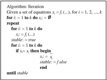
There is one such equation for each state q of M and each nonterminal A of G. The above set of equations can be solved using an iteration algorithm. Initially, assume {q} ⊕

A = Ofor each q and each A. Then, we can repeatedly evaluate the set of equations until a stable solution is reached. The iteration algorithm is shown in Fig. 2, where an expression, such as {q} ⊕ A , is treated as a variable.

Example: Fig. 3(b) is the ⊕ operator applied to the characteristic output machine shown in Fig. 1(d) and the context-free grammar in Fig. 3(a). For the sake of brevity, we have omitted the set symbols {……}. From the definition of the ⊕ operator, we obtain the following six equations:

Fig. 2. The iteration algorithm.

Algorithm: Iteration

Given a set of equations xi = fi (...), for i = 1, 2, ..., k

for i: = 1 to k do xi: = O repeat for i: = 1 to k do xi: = fi (...) stable: = true for i: = 1 to k do if xi= xi then begin xi: = xi stable: = f alse end until stable

{ } ({ } ) ({ } ) ({ } ) ({ } ) ({ } ) ({ } ) ({ } ) ({ } ) { } { } ({ } ) ({ } ) ({ } ) 1 1 1 1 1 1 1 2 1 1 2 2 2 2 ⊕ = ⊕ ∪ ⊕ ∪ ⊕ = ⊕ ⊕ ⊕ ∪ ⊕ ⊕ ⊕ ∪ ⊕ = ⊕ ⊕ ∪ ⊕ ⊕ ∪ ⊕ = ⊕ ∪ ⊕ ∪ ⊕ = T T T T T T T T T T µ µ ξ ξ θ µ µ ξ ξ θ µ ξ µ µ ξ ξ θ ({({ } ) ({ } ) ({ } ) ( ) ({ } ) { } { } ({ } ) ({ } ) ({ } ) ({ } ) ({ } ) ({ } ) ( 2 2 2 1 1 3 3 3 3 3 3 3 ⊕ ⊕ ⊕ ∪ ⊕ ⊕ ⊕ ∪ ⊕ = ⊕ ⊕ ∪ ⊕ ⊕ ∪ ⊕ = ⊕ ∪ ⊕ ∪ ⊕ = ⊕ ⊕ ⊕ ∪ ⊕ ⊕ ⊕ ∪ ⊕ = µ µ ξ ξ θ µ ξ µ µ ξ ξ θ µ µ ξ ξ θ T T T T T T T T T ⊕ ⊕ ∪ ⊕ ⊕ ∪ ⊕ = ⊕ = ⊕ ⊕ ⊕ = ⊕ = ⊕ ⊕ ⊕ = ⊕ = ⊕ ⊕ T T S T T S T T S T T µ) ( ξ) { } { } { } { } { } { } { } { } { } 1 1 1 2 2 2 3 3 3 $ $ $ $ $ $.

Let x1,x2,x3,x4,x5, and x6 denote the six terms: {1} ⊕ T, {2} ⊕ T, {3} ⊕ T, {1} ⊕ S, {2}

⊕ S, and {3} ⊕ S, respectively. After some simplification, we get the following six equations:

x x x x x x x x x x 1 2 1 2 1 3 4 1 2 3 1 1 = ⊕ ∪ ⊕ ∪ = ⊕ ∪ = = ⊕ = ⊕ = ⊕ ( ) ( ) { } ( ) { } µ ξ ξ $ x $ x $. 5 6

Initially, assume that x1 = x2 = x3 = x4 = x5 = x6 = O. We can repeatedly evaluate the six equations. After three iterations, we reach a stable solution: {1}⊕ S = {3}, {2} ⊕ S = {3},

{3} ⊕ S = O, {1} ⊕ T = {1,2}, {2} ⊕ T = {1}, and {3} ⊕ T = O.

Fig. 3. A context-free grammar and the ⊕ operator.

(a) A context-free grammar G (b) the ⊕ operator P1: S → T $ P2: T → µT µ P3: T → ξT ξ P4: T → θ ⊕ µ ξ θ $ T S 1 2 1 1 3 1,2 3 2 O 1 1 3 1 3 3 O O O O O O

The algorithm in Fig. 2 always halts due to its accumulative nature. That the solution is correct can be proved by inductive reasoning as follows: the addition of a state q′ into the solution of {q} ⊕ A can be traced backward, eventually to a transition q1 → a q2, where a is a token, in the finite-state machine. Thus, we can construct a string of terminals that is derivable from A, and that moves the finite-state machine from state q to state q′.

An application of the ⊕ operator is to decide whether a regular language and a con-text-free language intersect. A classical method for this problem is to integrate the finite-state machine of the regular language and the pushdown automaton of the context-free language into a new pushdown automaton. A new context-free grammar can then be de-rived from the integrated pushdown automaton. By contrast, with the ⊕ operator, the regu-lar language and the context-free language intersect if and only if the set {q0} ⊕ S, where q0 is the initial state of the finite-state machine of the regular language, and S is the start symbol of the context-free grammar, contains an accepting state of the finite-state machine. Though the ⊕ operator does not compute the exact intersection, it provides additional in-formation relating the states of a finite-state machine to the nonterminals of a context-free grammar. This information is useful in simplifying the LR parser of the context-free gram-mar as well as the gramgram-mar itself.

4. SIMPLIFYING THE GRAMMARS AND THE PARSERS

s on input α. Formally, L(s) is defined by the following context-free grammar Gs : S →α1 | α2 |...., where S is a new nonterminal not occurring in G, and α1,α2,....are the labels on all the distinct paths from the initial state to state s in CFSM(G). Gs also contains all the A-productions of G if the nonterminal A occurs in any of α1,α2,... Similarly, Gs contains all the B-productions of G if the nonterminal B occurs in any of the A-productions, etc. Note that L(s) is also a context-free language.

Given the regular expression defining a scanner, let M be the characteristic output machine of the scanner. Let Q be a set of states of M and s be a state of CFSM(G). Define

τ(Q,s) = ∪ {{q} ⊕ α | q ∈ Q, α ∈ L(s)}. Intuitively, τ (Q, s) denotes the set of possible final states of M when M, starting from a state in Q, scans a string of L(s). Set union ∪ may be distributed over the function τ : τ(Q1∪ Q2, s) = τ(Q1, s) ∪τ(Q2, s). Note that τ(O, s) = O. We can compute the τ function as follows: Let t1→x1 s,t2→x2 s,...., tk→xk s be all the incoming edges of state s in CFSM(G), where x1, x2, …, xk are either terminals or nonterminals. Note that L(s) = L(t1) • {x1} ∪ L(t2) • {x2} ∪ ... ∪ L(tk) • {xk},where • is defined as follows: A • B = {αβ | α ∈ A, β ∈ B} and αβ is the concatenation of the two strings α and β. Then, τ(Q, s) = (τ(Q, t1) ⊕ x1) ∪ (τ(Q, t2) ⊕ x2).... ∪ (τ(Q, tk) ⊕ xk).

In order to compute the values of τ({q}, s) for each state q of M and each state s of

CFSM(G), we can set up an equation for τ({q}, s). Then, an iteration algorithm similar to the one in the previous section can be applied. Initially, let τ({q}, s0) = {q}, where s0 is the initial state of CFSM(G). (The reason is that the empty string ε ∈ L(s0) and {q} ⊆ {q} ⊕ ε.) Let τ({q}, s) =O for all other states s. We can then evaluate the set of equations defining

τ repeatedly until a stable solution is obtained. Note that in computing τ({q},s), we can make use of the ⊕ operator obtained in the previous section.

The τ function can be used to remove redundant states and transitions from CFSM (G). Let q0 be the initial state of M. First, let s be a state of CFSM(G). If τ({q0}, s) =O, the state s is not reachable during parsing and, hence, can be removed. Secondly, let t →x _{s be} an edge in CFSM(G). If τ({q0}, t) ⊕ x = O, the transition t →x s can never be followed during parsing and hence can be removed as well. The removal of redundant states and transitions may render certain productions of the context-free grammar useless. These useless productions can be deleted. The removal of states, transitions, or productions may also reduce the size of the parse table. The technique presented here can be applied not only to CFSM(G), but also to LR(k) machines for any k and to LL parsers.

Note that the removal of states and transitions from CFSM(G) depends on the con-straints placed on the input to the parser, which is the output from the scanner. The output from the scanner is characterized by the characteristic output machine of the scanner. On the other hand, if the input to the parser is an arbitrary stream of tokens, no states and transitions can be removed.

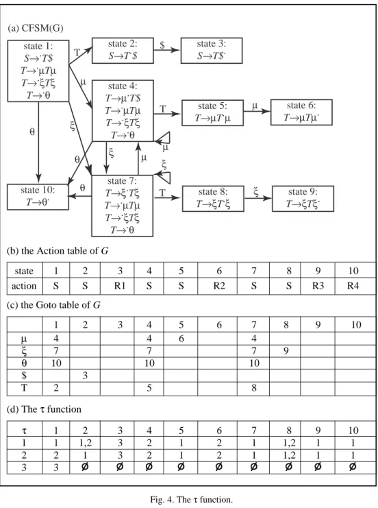
Example: Fig. 4(a) is the characteristic finite-state machine of the grammar in Fig. 3(a).

Figs. 4(b) and (c) are the action and goto tables. Fig. 4(d) is the τ function on the COM in Fig. 1(d) and the characteristic finite-state machine in Fig. 4(a). We have omitted the set symbol {…} in Fig. 4 for the sake of brevity. The equations defining the τ function on state 1 are as follows: τ τ τ τ τ τ τ µ τ µ τ µ τ τ τ τ µ τ τ ξ ({ }, ) { } ({ }, ({ }, ({ }, ({ }, ({ }, ({ }, ({ }, ({ }, ({ }, ({ }, ({ }, ({ }, ({ }, ({ }, 1 1 1 1 1 1 1 1 1 1 1 1 1 1 1 1 1 2) = 1) 3) = 2) 4) = ( 1) ) ( 4) ) ( 7) ) 5) = 4) 6) = 5) 7) = ( 1) ) = ⊕ ⊕ ⊕ ∪ ⊕ ∪ ⊕ ⊕ ⊕ ⊕ ∪ T T $ (( 4) ) ( 7) ) 8) = 7) 9) = 8) 10) = ( 1) ) ( 4) ) ( 7) ). τ ξ τ ξ τ τ τ τ ξ τ τ θ τ θ τ θ ({ }, ({ }, ({ }, ({ }, ({ }, ({ }, ({ }, ({ }, ({ }, ({ }, 1 1 1 1 1 1 1 1 1 1 ⊕ ∪ ⊕ ⊕ ⊕ ⊕ ∪ ⊕ ∪ ⊕ T

The equations are solved using an iteration algorithm similar to that in Fig. 2. The τ function for other states of M is computed similarly. Consider the edge e from state 4 to itself labeled µ in Fig. 4(a). Intuitively, the edge e is traversed only when the scanner produces two consecutive µ’s. Since the scanner in Fig. 1 can never produce two consecu-tive µ’s, that edge can be eliminated from the parser. Formally, the edge e may be removed because τ({1}, 4) ⊕ µ = O.

Example: Suppose the definition of the token ξ is changed to bb*. In this case, the scanner would not be able to produce two consecutive ξ’s. Hence, the edge from state 7 to itself in

5. A LATTICE FRAMEWORK FOR ANALYZING

CONTEXT-FREE LANGUAGES

Let G = (N, T, P, S) be a context-free grammar. Let LG be the language defined by G. We may wish to compute certain collective properties of LG based on a mapping M : T*→ _F′_{, where F}′ _{is the domain-of-interest (M maps individual strings of terminals into the}

Fig. 4. The τ function.

(a) CFSM(G) state 1: S→.T$ T→.µTµ T→.ξTξ T→.θ _Tstate 4:_→µ._T$ T→.µTµ T→.ξTξ T→.θ state 2: S→T.$ state 7: T→ξ.Tξ T→.µTµ T→.ξTξ T→.θ state 10: T→θ. state 3: S→T$. state 5: T→µT.µ state 6: T→µTµ. state 8: T→ξT.ξ state 9: T→ξTξ. T T T $ µ θ θ θ µ µ µ ξ ξ ξ ξ

(b) the Action table of G

state 1 2 3 4 5 6 7 8 9 10

action S S R1 S S R2 S S R3 R4

(c) the Goto table of G

1 2 3 4 5 6 7 8 9 10 µ 4 4 6 4 ξ 7 7 7 9 θ 10 10 10 $ 3 T 2 5 8 (d) The τ function τ 1 2 3 4 5 6 7 8 9 10 1 1 1,2 3 2 1 2 1 1,2 1 1 2 2 1 3 2 1 2 1 1,2 1 1 3 3 O O O O O O O O O

domain-of-interest). For instance, M may be taken as the length function (i.e., by comput-ing the length of a strcomput-ing), and we want to know whether all sentences of LG are of even length. Since LG is, in general, infinite, it is not possible to compute the collective proper-ties by enumerating the sentences of LG one by one. The lattice framework proposed in this section provides us with a feasible way to compute the collective properties.

Assume that the domain-of-interest F′ can be embedded into (or is closely related to) a finite (see problem 6 below) lattice (F, ≤). Let B and A be the join and meet operations, respectively. The least element and the greatest element of F are denoted by fmin and fmax, respectively. M is modified and extended accordingly so that M maps strings of terminals and nonterminals to s of F, and M satisfies the following property: M(αβ) =M(α) ⊗ M(β), where ⊗ is an associative and monotone operation on F with an identity element e (that is, if a ≤ b, then a ⊗ c ≤ b ⊗ c, c ⊗ a ≤ c ⊗ b, and c ⊗ e = e ⊗ c = c, for all c ∈ F). (Under the

above conditions, M(ε) = e, here ε isthe empty string.) As a notational convenience, M(α) will be written as fα. fα represents the collective properties of {β | β ∈ T *, α→ *β}.

For each a ∈ T, we may compute its image fa in F directly. In order to compute fα, where α ∈ (N ∪ T)*_{, we need to find f}

A for each A∈ N. Since A may be viewed as the set of terminal strings LA that are derivable from the nonterminal A through the production rules of G, the production rules of G define the relationships among these context-free languages

LA. These relationships (or production rules) are translated into equations in F as follows: For each A∈ N, the set of all the A-productions A→ α | β |… is translated into the equation

fA = hα♦ hβ♦...., where hα = H(α, fα) for a function H that is monotone in its second argument. H is monotone in the sense that if f ≤ f′, then H(α, f ) ≤ H(α, f′ ) for all strings

α ∈ (N ∪ T)*_{. The} ♦ _{operator is called the luence operator, which may be either} B or A. We also require that ♦ be distributive over ⊗, that is, f ⊗ (h1♦ h2) = (f ⊗ h1) ♦ (f ⊗ h2) and (h1♦ h2) ⊗ f= (h1⊗ f ) ♦ (h2⊗ f ). Let f♦be the identity element of ♦, namely, f♦ = fmin if

B is the confluence operator; f♦ = fmax if A is the confluence operator. It is also required that f ♦ f♦ = f♦♦ f = f for all f ∈ F. Then we can solve this set of equations using the iteration

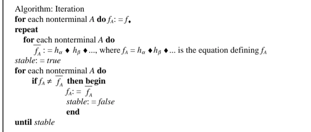
algorithm in Fig. 5, where, for each A ∈ N, the initial value of fA is f♦.

Fig. 5. The iteration algorithm.

Algorithm: Iteration

for each nonterminal A do fA: = f♦

repeat

for each nonterminal A do

A

f : = hα♦ hβ ♦..., where fA = hα ♦hβ ♦... is the equation defining fA stable: = true

for each nonterminal A do if fA≠ f then begin_A

fA: = f_A stable: = false

end until stable

Let B = {fa| a ∈ T}. B, the collection of the images of terminals in the lattice, repre-sents the basic building blocks of the framework. The five components F, ⊗, B, H, and ♦ consist of an analysis scheme of a context-free grammar. The detailed definition is delayed until the next section. In this section, we will examine several examples to show the many applications of the lattice frameworks.

That the iteration algorithm always halts with a stable solution can be demonstrated as follows. For each A∈ N, let fA,j be the value for A at the end of the jth iteration. Let fA,j+1 be the value for A at the end of the j+1st _{iteration. Since H,} ⊗_{, and} B (or A) are monotone, and the iteration algorithm starts from fmin (or fmax, respectively), fA,j≤ fA,j+1 (or fA,j+1≤ fA,j, respectively) for every A∈ N. Since F is a finite lattice, the iteration algorithm always halts

with a stable solution. (We will show that the stable solution is correct in the next section.) Let S be the start symbol of the grammar G. In general, fs is the intended result. Sometimes, we might be interested in fα for some string α. It is straightforward to compute

fα once fA, for each A∈ N, is known. We can gain insight into properties of the string α through its image, fα, in F.

The essence of the framework is to compute some values, such as fsor fα, that cannot be computed directly. Note that there are subtle relationships (induced by the production rules of the grammar) between the values that interest us and certain closely related values. If the domain-of-interest can be embedded in a finite lattice with appropriate ⊗, ♦, and H functions, the values that interest us can be computed together with the closely related values using the iteration algorithm. This technique is similar to some inductive proofs in that, sometimes, we need to strengthen the induction hypothesis (that is, in order to prove a stronger result than is actually needed). In what follows, we will list several problems that can be solved in a lattice framework.

Problem 1: In Section 3 of this paper, we try to decide whether a regular language and a

context-free language have common elements. Our strategy is to feed each sentence of the context-free grammar into the finite-state machine R of the regular language and examine the final states of R, that is, the set {q | R moves from its initial state to state q on input β, where β is a sentence of the context-free language}. The regular language is transformed into a finite-state machine R. Let Q be the set of states of R. Let F={f:2Q→ ₂Q _{| f(}O)=O, f (Q1∪ Q2)=f(Q1)∪ f(Q2), Q1⊆ Q, Q2⊆ Q}. Elements of F are ordered as follows: Let f1 and f2 be two elements of F. f1≤ f2 if and only if, for all Q′⊆ Q, f1(Q′) ⊆ f2 (Q′). The least element of F is λe. O, and the greatest element is λe. if e = O, thenO, else Q. Hence, (F, ≤

) is a lattice. Note that function composition ° on F is associative and monotone and has an identity element λe. e. For each α∈ (N ∪ T)*_{, let f}

α be the “extended” state transition

function of R as defined below: For any terminal symbol a, fa is the element of F that is uniquely determined from the row (corresponding to a) of the state transition table of R. For , α, β∈ (N ∪ T)*_{, f}

αβ = fβ _{° f}α. For each nonterminal A of the context-free grammar, the set

of all the A-productions A→α | β |….is translated into the equation fA = fαB fβB …. Now, the problem is cast in a lattice framework. We can use the iteration algorithm to find solutions for fA. Finally, we are interested in fs ({q0}), where q0 is the initial state of R, and S is the start symbol of the context-free grammar. Note that, in this framework, fα = λe. (e ⊕α) in Section 3.

Problem 2: In Section 4 of this paper, we attempted to simplify a context-free grammar G

and its parser with information provided by the COM of the scanner. The lattice frame-work is applicable to this problem as well. Let G = (N, T, P, S). The characteristic finite-state machine CFSM(G) of grammar G is transformed into a regular grammar G as follows. Each state s of CFSM(G) corresponds to a nonterminal S in G. Each transition t →xs in CFSM(G) corresponds to a production rule S→T x in G. An additional production rule

u

U→ is added to G, where U corresponds to the initial state of CFSM(G), and u is a new terminal symbol in G. The start symbol X of G corresponds to the accepting state of CFSM(G). The lattice F is the same one as in Problem 1. Note that the set of terminal

symbols of G is N ∪ T ∪ {u}. For x ∈(N ∪ T), let fx be the one computed in Problem 1. Let fu = λe.e. Define fαβ = fβ ° fα, where ° is defined in Problem 1. For each nonterminal S in G, the set of all the S-productions, S→α | β |...., is translated into the equation

f

=

S fα

B fβB ... Now, the problem is cast in a lattice framework. We can use the iteration

algorithm to find solutions for fS for each nonterminal S of G. Finally, we are interested

in fX, where X is the start symbol of G. Note that, in this framework, f_S(Q)=τ(Q,s),

where s is a state of CFSM(G).

Problem 3: Suppose we want to decide whether the lengths of all the sentences of a

con-text-free language are multiples of 3. We can use the lattice framework to solve this problem. Let F be the powerset of the set {0,1,2}. (F, ⊆) is a lattice. Define fαβ = fα• fβ, where s • t

= {(a+b) mod 3|a ∈ s,b∈t}. Note that

•

Problem 4: (erasable nonterminals) Suppose we want to know whether a nonterminal A

can derive the empty string. Let F={⊥, T}, with ⊥ ≤ T. Now define M as follows. For each terminal symbol a, fa =⊥. Let fαβ = fαA fβ. Note that fε = T. The set of all the A-productions A → α | β |…. is transformed into the equation fA = fαB fβB ... Then, we can solve the equations using the iteration algorithm. The initial value of fA, for each nonterminal A, is ⊥. Finally, fA = T if and only if A→*ε.

Problem 5: (non-empty languages) A context-free language is non-empty if it can derive at

least one sentence. This problem can also be solved in the lattice framework. Let F={⊥, T}, with ⊥ ≤ T. Define M as follows. For all terminal symbols a, fa = T. Let fαβ = fαA fβ. Note that fε = ⊥. The set of all the A-productions A → α | β |…. is transformed into fA = fαB fβ B.... Then, we an solve the equations using the iteration algorithm. The initial value for

fA, for each nonterminal A, is ⊥. Finally, fS = T if and only if the language is non-empty, where S is the start symbol of the grammar.

Problem 6: (context-free languages) Let G = (N, T, P, S) be a context-free grammar. Let T* be the set of all the strings of symbols from a vocabulary T. Let F be the powerset of T*_. The elements of F are ordered by means of subset containment. Note that (F, ⊆) is an (infinite) lattice. Let fa = {a}for each a ∈ T. Let fαβ = fα∇ fβ , where s1∇s2 = {t1t2|t1∈ s1, t2

∈ s2}. Note that ∇ is associative and monotone and has an identify element {ε}. Hence, fε = {ε}. For each A∈ N, the set of all the A-productions A → α | β |… is translated into the equation fA = fα∪ fβ ∪.... For each A ∈ N, the initial value for fA is O. In this example, fA is the set of terminal strings derivable from the nonterminal A by the production rules of G. Since the lattice is infinite, the iteration algorithm can not terminate. However, any element of fA, for any nonterminal A, can be generated in a finite number of iterations. Let S be the start symbol of the grammar. fS = LG. (This example is essentially the same as the one in [5].)

Problem 7: The essential nonterminals of a context-free grammar G are those that are used

in the derivation of every sentence of LG. Assume that G contains no useless symbols. Let F be the powerset of N (where N is the set of nonterminals of G). Elements of F are ordered

by means of subset containment. Now, define M as follows. Let fa = O for all terminals a. Let fαβ = fα∪ fβ . Note that fε = O. For each nonterminal A, the set of all the A-productions

A →α | β |….| is transformed into the equation fA = (NONTERM (α) ∪ fα) ∩ (NONTERM (β) ∪ fβ) ∩...., where NONTERM(α) is the set of all nonterminals in α. For each nonterminal

A, the initial value for fA is N. We can solve for fA using the iteration algorithm. Finally, {S}

∪ fS, where S is the start symbol of G, is the set of essential nonterminals.

Problem 8: (shortest-path problem) This problem is adapted from [6]. Given a directed

graph in which each edge carries a non-negative distance, we wish to compute the shortest distance from a starting node s to all other nodes. The graph is transformed into a context-free grammar as follows. Each node a corresponds to a nonterminal A. Each edge a →e _b (where e is the identity of the edge in the graph) corresponds to a production rule B → Ae,

where e is a new terminal symbol in the grammar. The starting node s induces an additional rule S → ε. Let F be R+ _{= R} ∪_{∞_}(where ∞ _{is a positive infinite large number). Let f}

e be the distance carried by the edge e. Let fαβ= fα + fβ. Let the confluence operator be the minimum

function. Then, fA, for each nonterminal A, is the shortest distance from node s to node a in the given graph.

Problem 9: (data-flow analysis) Many data-flow analysis problems can be cast in lattice

frameworks. We will demonstrate this application using an interprocedural data-flow analysis problem, taken from [4]. Assume that there are several procedures that call one another in a program. We wish to compute Use(A), the set of variables that may be used directly or indirectly during a call to procedure A. Let F be the powerset of the set of variables in the program, with ∪ and ∩ as the join and meet operators.For each procedure A, there is a nonterminal A and a terminal a in the associated grammar. For each nonterminal A, the set of all the A-productions is A → a | α…, where α = B1B2.... and B1B2.... are all the procedures

that can be called directly by procedure A. The set of all the A-productions is translated into the equation fA = fa∪ fα (that is, ∪ serves as the ♦ operator). Let fαβ = fα∪ fβ (that is, also serves as the ⊗ operator). Finally, for each terminal a, let fa= LocalUse(A), the set of variables that can be used locally in procedure A. Then we can solve the equations with the iteration algorithm. Note that the equation defining Use(A) in [4] is Use(A)= LocalUse (A) ∪ (∪ B is calledby A Use(B)). A similar lattice can be used to solve the Def(A), the set of

6. ANALYSIS SCHEMES

We will now formalize the notion of a lattice framework and discuss the fundamental properties of a framework.

Defintion: An analysis scheme Ω is a 5-tuple (F, ⊗, B, H,♦), where F is a lattice with a join B and a meet A operation, ⊗ is an associative and monotone operation on F with an identity element, B = {fa | a is a (terminal) symbol of the context-free language to which the scheme is applied}, H is a monotone (in its second argument) function that maps a string (of termi-nals and nontermitermi-nals) and an element of F to an element of F (H is monotone in its second argument in the sense that if f ≤ f′, then H(α, f) ≤ H(α, f′), for all strings α), and ♦ is either B or A. Let f♦ be the identity element of ♦. ♦ and ⊗ satisfy the following three axioms: (1)

f ⊗ (h1♦ h2) = (f ⊗ h1) ♦ (f ⊗ h2), (2) (h1 ♦ h2) ⊗ f = (h1⊗ f) ♦ (h2⊗ f), and (3) f ⊗ f♦ = f♦

⊗ f = f♦.

To apply an analysis scheme Ω = (F, ⊗, B, H,♦) to a context-free grammar G = (N,

T, P, S), we first translate, for each A∈ N, the set of all the A-production rules A → α | β |…. into the equation fA = H (α, fα) ♦ H(β, fβ) ♦…, where fµξ is an abbreviation of fµ ⊗ fξ, for µ,

ξ ∈ (N ∪ T)*_{. The iteration algorithm in Fig. 5 is used to compute the value of f} A. The initial value for fA , for each A∈ N, is f♦, the identity element of ♦. The result of the analysis is fS, where S is the start symbol of grammar G.

An analysis scheme is applied to context-free grammars. We can check that all of the above problems make use of analysis schemes. There might be other constraints as to the kinds of context-free grammars and languages to which an analysis scheme is applicable. For instance, the analysis scheme in Problem 7 is applicable only to grammars having no useless symbols. These constraints are considered to be outside the schemes.

An analysis scheme can be used to compute the properties of both context-free

lan-guages and context-free grammars. For instance, Problems 1 through 6 are concerned with

languages whereas Problem 7 is concerned with grammars. A common characteristic of Problems 1 through 6 lies in the H function, where H(α, f) = f. By contrast, in Problem 7, H(α, f) depends not only on f, but also on α, (Note that α is the right-hand-side of a produc-tion rule.) This distincproduc-tion is reasonable in that the properties of a context-free language should not depend on any particular choice of grammar. Hence, we can derive the follow-ing definition.

Definition: An analysis scheme is called a language-analysis scheme if H(α, f) = f. It is

called a grammar-analysis scheme otherwise.

This definition raises an interesting question: Since a context-free language may be defined by more than one context-free grammar, does a language-analysis scheme always compute the same answer no matter which context-free grammar is used in the computation? We will use a lemma to make this a claim. (In what follows, the notation ♦S denotes the

value of s1♦s2♦…, where s1, s2…. are all the elements of S. Since ♦ is commutative and associative, the order of elements is not significant.)

Lemma 1: Suppose that a language-analysis scheme is applied to a context-free grammar

Proof: Let fA,k be the value for the nonterminal A after the kth iteration of the loop in the iteration algorithm in Fig. 5. Note that fA = fA,∞ = fA,k, for some finite k, since the iteration algorithm reaches a stable solution after a finite number of iterations. We can prove by induction on k that fA,k = ♦ {fα | α∈T*, the height of the derivation tree of A→ *α is at most k}. For the sake of clarity, we assume that the confluence operator ♦ is B in the proof. A parallel argument applies if A is the confluence operator.

Base case. Let k = 1. Consider any nonterminal A, which is defined by the equation fA = fα1

B fα2 B. In the computation of fA,1, if α i contains any nonterminals, fαi = fmin (due to the properties of ⊗ and fmin in the analysis scheme). This term is dropped from the above equation since fmin B x = x B fmin = x for any x. Therefore, fA,l = B {fα|A →α is a production and α ∈ T*_}.

Induction hypothesis. Assume that, for k < m and for any nonterminal A, fA,k = B {fα |α∈

T*_{, the height of the derivation tree of A}→ *α _{is at most k }.}

Induction step. We need to prove that, for any nonterminal A, fA,m = B {fα | α ∈ T*, the

height of the derivation tree of A→*α _{is at most m}.}

Consider any nonterminal A, which is defined by the equation fA = fα1B fα2 B... Note that, in the computation, fA,m = fα1,m-1B fα2,m-1 B.... (The notation fαi,m-1 means that, for any nonterminal B in αi, fB,m-1 will be used for fB.) If α i contains a nonterminal, say B, then αi may be written as γBδ. Because ⊗ is associative, fαi,m-1 = fγ,m-1⊗ fB,m-1 ⊗fδ,m-1. By the induction hypothesis, fB,m-1 = B {fβ | β∈ T*, the height of the derivation tree of B → ∗β is at most m-1}. Thanks to the distributive law of B over ⊗, fαi,m-1 = B{fγ,m-1⊗ fβ ⊗ fδ,m-1 | β ∈ T*, the height of the derivation tree of B →*β _{is at most m-1}. By applying the same argument} to all nonterminals in γ and δ, we know that fαi,m-1 = B {fµ | µ ∈ T*, the height of the derivation tree of A→αi→*µ _{is at most m}. Since the equation f}

A = fα1B fα2B... is translated from the set of all the A-productions, any string µ ∈ T* _{such that the height of the} derivation tree A→*µ _{is at most m is considered in one of f}

αi,m-1. Therefore, fA,m = B{fµ | µ

∈ T*_{, the height of the derivation tree of A}→ *µ _{is at most m}. This completes the induction} proof.

The following theorem asserts that, if a language-analysis scheme is used to compute the properties of a context-free language, the result computed by the scheme does not de-pend on the particular choice of context-free grammar. The theorem is a corollary to the above lemma.

Theorem 1: (Soundness of language-analysis schemes) Assume that the context-free

gram-mars G and G define the same context-free language. Let S and S be the start symbols of

G and G, respectively. Then, the results obtained by applying a language-analysis scheme to G and G are the same. That is, f_S= f_S.

Definition: Let Ω be a language-analysis scheme. Let L be a context-free language. The notation Ω(L) means fS, where S is the start symbol of a context-free grammar defining L.

Below, we list several fundamental properties of language-analysis schemes. The proofs of these theorems are based on Lemma 1 and are easy enough to be omitted.

Theorem 2: Let Ω be a language-analysis scheme. Let L and M be context-free languages.

Ω(L ∪ M) = Ω(L) ♦Ω (M).

Theorem 3: Let Ω be a language-analysis scheme. Let L and M be context-free languages. Assume that L ⊆ M. If B is the confluence operator, Ω(L) ≤ Ω(M). If A is the confluence operator, Ω(L) ≥ Ω (M).

Theorem 4: Let Ω be a language-analysis scheme. Let L and M be context-free languages. If B is the confluence operator, Ω(L ∩ M) ≤ Ω(L) A Ω(M). If A is the confluence operator,

Ω(L ∩ M) ≥ Ω(L) B Ω(M).

Theorem 5: Let Ω be a language-analysis scheme. Let L and M be context-free languages.

Ω(LM) = Ω(L) ⊗ Ω(M). (LM is a language consisting of the concatenation of a sentence of

L and a sentence of M.)

Theorem 6: Let Ω be a language-analysis scheme. Let L be a context-free language. Ω(L*₎ = ♦{ Ω(L)k _{| k} ≥ _{0 }, where} Ω_(L)0 _{is the identity element of} ⊗ _and Ω_(L)k+1 ₌ Ω_(L) ⊗ Ω_(L)k_. (L* _{is a language consisting of the concatenation of zero or more sentences of L.)}

Theorem 7: Let Ω be a language-analysis scheme. Ω({ε}) = the identity element of ⊗.

Theorem 8: Let Ω be a language-analysis scheme. Ω(O) = f♦, the identity element of ♦.

We will now turn to another important characterization of language-analysis schemes: any difference between two context-free languages is witnessed by a language-analysis scheme. The essence of this characterization lies in the condition that the lattice F in a language-analysis scheme is finite. If we can use infinite lattices, the following theorem is trivial. The scheme in Problem 6 in the previous section is the witness. It is not so obvious if F must be finite.

Theorem 9: Let L and M be context-free languages. Assume that L ≠ M. Then, there is a

language-analysis scheme Ω such that Ω(L) ≠ Ω(M).

Proof: Since L ≠ M, without loss of generality, we may assume that there is a sentence α ∈ L but α ∉ M. Let j be the length of α. If j = 0, the scheme in Problem 4 is the witness. Assume j > 0. Let k = j+1.

We will now construct a language-analysis scheme Ω, as follows: Let T ≤ k _{= {}α | α

∈T*_{, the length of} α _{is at most k}. Let F be the powerset of T} ≤ k_{. Elements of F are ordered} by means of subset containment. Let fαβ = fα ∆ fβ , where f1 ∆ f2 = {firstk(t1t2) | t1∈f1, t2∈ f2} and firstk(t) computes the first k symbols of the string t. It can be shown that ∆ is associa-tive and monotone and has an identity element {ε}. For a ∈ T, let fa = {a}. Let ∪ be the confluence operator. Hence, f♦ = O. It can be verified that ∪ and ∆ satisfy the following

three axioms: (1) f ∆ (h1∪ h2) = (f ∆ h1) ∪ (f ∆ h2), (2) (h1∪ h2) ∆ f= (h1 ∆ f) ∪ (h2∆ f), and (3) f∆O = O ∆ f= O. In essence, Ω(L) = {firstk(t) | t ∈ L }. We can see that α ∈ Ω (L) but α ∉ Ω(M).

Corollary 1: Let L and M be context-free languages. If Ω(L) = Ω(M) for all language-analysis schemes Ω, then L = M.

7. LANGUAGE-ANALYSIS SCHEMES BASED ON

INFINITE LATTICES

The requirement that F be a finite lattice in an analysis scheme can be relaxed. Finite-ness is used to guarantee termination of the iteration algorithm. The iteration algorithm also terminates for the class of finite-height lattices, in which the longest path from fmax to fmin is of finite length.

It is interesting to briefly investigate the case where F in a language-analysis scheme is infinite. The main problem with infinite lattices is that the iteration algorithm can not terminate. However, we can show that termination is an inherent property of context-free languages. That is, termination is independent of the particular grammar used to describe the language.

Theorem 10: Let Ω be a language-analysis scheme based on an infinite lattice. Suppose that grammars G1 and G2 define the same language. The application of Ω to G1 terminates if and only if the application of Ω to G2 terminates. Furthermore, when the applications terminate, the applications yield the same values.

Proof: Let L be the language defined by G1 (or, equivalently, G2). Suppose that the appli-cation of Ω to G1 terminates after k1 steps. Let L1 = {α | α ∈ L and the height of the derivation tree of α based on G1 is at most k1}. Since the application of Ω to G1 terminates after k1 steps, ♦{fα | α∈ L1} = ♦ {fα | α ∈ L}. Furthermore, L1 is finite. Let k2 = max { h | h is the height of the derivation tree of α based on G2, where α∈ L1}. Let L2 = {β | β∈ L and the height of the derivation tree of β based on G2 is at most k2}. Note that L1⊆ L2 ⊆ L. Because ♦ is monotone, we have ♦ {fα | α ∈ L1} = ♦ {fα | α ∈ L2} = ♦ {fα | α ∈ L}. This implies that the application of Ω to G2 will terminate by at most k2 steps.

Once we know that the application of terminates, the properties listed in the previous section all hold.

8. CONCLUSIONS AND RELATED WORK

We have characterized a lattice framework for analyzing context-free grammars and context-free languages. This lattice framework is motivated by a technique for simplifying parsers using information derived from the associated scanners and can be used in many other applications, including data-flow analysis. The crux of the lattice framework is to view the → symbols in the production rules of grammars as defining equations of closely related entities. When the domain-of-interest is a finite lattice, the equations can be solved using an iteration algorithm. An introduction to lattice theory can be found in [7].

The lattice framework can be viewed as a form of induction [8]. (This is no surprise at all since context-free grammars are an inductive definition of context-free languages.) Imagine that we want to prove a property of a context-free language P(L). We may not be able to prove it directly if P(L) alone is the induction hypothesis. Sometimes, the proof proceeds smoothly when we strengthen the induction hypothesis to PA _(L

A) and PB (LB)

and…., where A, B, … are all the nonterminals of a grammar defining L and PA _,PB_{,… are} properties closely related to P. Remember that LA are the strings of terminals that are derivable from the nonterminal A. This induction hypothesis means that, in order to prove that L has the property P, we actually need to prove that LA has the property PA, that LB has the property P B_{, etc. For instance, consider the language defined by the grammar} consist-ing of two production rules: S→aX and X→aS | a. Now, we want to prove that all sentences

of LS have even length. In an inductive proof, the induction hypothesis could be that all the

sentences of LS have even length and that all sentences of LX have odd length. This is exactly what a scheme similar to that in Problem 3 (in Section 5) will compute. The chal-lenge for an inductive proof is to find an appropriate induction hypothesis and to prove it. By contrast, in a language-analysis scheme, the difficulty lies in constructing an appropri-ate lattice. When such a lattice is constructed, the iteration algorithm automatically com-putes the “induction hypothesis” (which is fA, fB etc.).

Knuth’s work [6] was the first on computing properties of grammars. Our lattice framework differs from Knuth’s work in four aspects: (1) Knuth uses real numbers (R ∪ {∞}), which is a total order, whereas we allow general lattices; (2) Knuth’s algorithm trans-forms production rules into independent superior functions whereas we use a single opera-tor ⊗ to transform all the productions; (3) Knuth’s superior functions need to satisfy an additional constraint viz, the value of a function application must be at least as large as any of its arguments; and (4) Knuth uses only the minimum function, which corresponds to the A operator, as the confluence operator. By contrast, our lattice framework uses B as well as A as the confluence operator. On the other hand, because Knuth assumed certain prop-erties that allow him to adopt a generalization of Dijkstra’s shortest-path algorithm, Knuth’s work was particularly efficient. Moencke and Wilhelm [9]developed a theory similar to the work reported for flow analysis in attribute grammars. Their work extends Knuth’s in that they employ partial orders, rather than total orders. Ramalingam in his thesis [10] pointed out that interprocedural dataflow analysis frameworks, such as [11], can be viewed as in-stances of grammar-analysis problems. In these problems, the grammar describes valid execution paths. Ramalingam’s work can be viewed as a generalization of Knuth’s and Moencke and Wilhelm’s results. All these researchers did not distinguish between guage-analysis and grammar-analysis schemes. We also address various properties of lan-guage-analysis schemes, in particular, the independence of the computation results with respect to the particular grammars used in the computation.

The lattice framework bears some similarity with denotational semantics [7]. In denotational semantics, each terminal symbol corresponds to a function, and ⊗ corresponds to a function application. One important difference lies in the fact that function application is not associative. By contrast, ⊗ is an associative operator in our framework. Another difference is that denotational semantics compute a property (that is, the meaning) of a sentence in the language whereas our framework computes a property of the (context-free) language.

This lattice framework is similar to some circular attribute grammars [12]: We may view fA , fB,.... as attributes of the nonterminals and fA = hα♦ hβ♦... as attribution equations. Clearly, this “attribute grammar” was circular in general. However, a finite-lattice frame-work guarantees that the iteration algorithm reaches a stable solution in a finite number of iterations.

The Mealy-machine description of a scanner is motivated by a study of the look-ahead problem in lexical analysis [13]. The technique for handling the look-look-ahead problem is similar, in spirit, to the pattern-matching algorithm of [14] and the string matching algo-rithm of [15].

ACKNOWLEDGMENT

The author wishes to thank Professor Thomas Reps of the University of Wisconsin, Madison, for many helpful discussions and for pointing out many related works.

REFERENCES

1. W. Yang, “Mealy machines are a better model of lexical analyzers,” Computer

Languages, Vol. 22, No. 1, 1996, pp. 27-38.

2. J.E. Hopcroft and J.D. Ullman, Introduction to Automata Theory, Languages, and

Computation, Addison-Wesley, Reading, MA, 1979.

3. A.V. Aho, R. Sethi and J.D. Ullman, Compilers: Principles, Techniques, and Tools, Addison-Wesley, Reading, MA, 1986.

4. C.N. Fischer and R.J. LeBlanc, Jr., Crafting a Compiler with C, Benjamin/Cummings, Reading, MA, 1991.

5. D. Mandrioli and C. Ghezzi, Theoretical Foundations of Computer Science, Addison-Wesley, Reading, MA, 1987.

6. D.E. Knuth, “A generalization of Dijkstra’s algorithm,” Information Processing Letters, Vol. 6, No. 1, 1977, pp. 1-5.

7. J.E. Stoy, Denotational Semantics: The Scott-Strachey Approach to Programming

Lan-guage Theory, MIT Press, Cambridge, MA, 1977.

8. R.M. Burstall, “Proving properties of programs by structural induction,” The Computer

Journal, Vol. 12, No. 1, 1969, pp. 41-48.

9. U. Moencke and R. Wilhelm, “Grammar flow analysis,” in Proceedings of the

Interna-tional Summer School SAGA, Lecture Notes in Computer Science, Vol. 545, 1991, pp.

151-186.

10. G. Ramalingam, “Bounded incremental computation,” Ph.D. dissertation TR-1172, Computer Science Deptartment, University of Wisconsin, 1993.

11. M. Sharir and A. Pnueli, “Two approaches to interprocedural data flow analysis,” in S. S. Muchnick and N.D. Jones (eds.), Program Flow Analysis: Theory and Applications, Prentice-Hall, Englewood Cliffs, NJ, 1981, pp. 189-223.

12. D.E. Knuth, “Semantics of context-free languages,” Mathematical System Theory, Vol. 2, No. 2, 1968, pp. 127-145. Correction, ibid., Vol. 5, No. 1, 1971, pp. 95-96. 13. W. Yang, “On the look-ahead problem in lexical analysis,” ACTA Informatica, Vol. 32,

1995, pp. 459-476.

Journal on Computing, Vol. 6, No. 2, 1977, pp. 323-350.

15. A.V. Aho and M.J. Corasick, “Efficient string matching: An aid to bibliographic search, ” Communication ACM, Vol. 18, No. 6, 1975, pp. 333-340.

Wuu Yang (¨Z) received his B.S. degree in computer

science from National Taiwan University in 1982 and the M.S. and Ph.D. degrees in computer science from the University of Wisconsin, Madison, in 1987 and 1990, respectively. Currently, he is an associate professor at National Chiao-Tung University, Taiwan, Republic of China. Dr. Yang’s research interests in-clude programming languages and compilers, attribute grammars, and parallel and distributed computing. He is also very interested in the study of human languages and human intelligence.