影像處理技術應用於透地雷達資料之研究

國

立

交

通

大

學

資訊科學與工程研究所

碩

士

論

文

影像處理技術應用於透地雷達資料之研究

A Study on Applications of Image Processing in

Ground Penetrating Radar Data

研 究 生：王慧縈

指導教授：薛元澤 教授

影 像 處 理 技 術 應 用 於 透 地 雷 達 資 料 之 研 究

A Study on Applications of Image Processing in Ground Penetrating Radar Data

研

究 生：王慧縈 Student：Hui-Ying Wang

指導教授：薛元澤 Advisor：Yuang-Cheh Hsueh

國 立 交 通 大 學

資 訊 科 學 與 工 程 研 究 所

碩 士 論 文

Submitted to Institute of Computer Science and Engineering College of Computer Science

National Chiao Tung University in partial Fulfillment of the Requirements

for the Degree of Master

in

Computer Science

June 2006

Hsinchu, Taiwan, Republic of China

i

影像處理技術應用於透地雷達資料之研究

學生：王慧縈

指導教授：薛元澤

國立交通大學資訊科學系﹙研究所﹚碩士班

摘要

近年來，透地雷達的非破壞性探測技術，被廣泛的應用於偵測地下管

線。由於台灣多為非均勻地質層，造成透地雷達影像中的非金屬管線影像

更容易受到影響而誤判。而低對比度的透地雷達影像，使得專家辨識管線

變的更為困難。增強弱化及低對比度的管線影像而不受整體影像中的雜訊

影響為主要研究方向。本論文嘗試使用數學形態學裡的形態交離轉換法及

運算拋物線及建立拫物線模型對管線影像偵測並做區域性的影像增強，使

得拋物線能有效與背景區分開來。觀察影像特徵後，設計幾組適用的形態

學結構元素做為偵測管線影像，再運用拋物方程式產生模型，以達成區域

性的影像增強。實驗結果顯示本論文提出的方法能有效提升管線解析度。

A Study on the Application of Image Processing

in the Ground Penetrating Radar data

Student: Hui-Ying Wang

Advisors: Dr.Yuang-cheh Hsueh

Institute of Computer and Information Science

National Chiao Tung University

ABSTRACT

Recently, technology of un-destructive exploring of GPR(Ground Penetrating Radar) is extensively applied in underground pipes detection. Since un-uniform of geology layer in Taiwan, it is easier to have erroneous judgment in nonmetal pipeline images made by GPR. And low contrast and weak GRP images make experts encounter more difficulties while identifying pipes. Meanwhile, low contrast GPR images make experts even harder to determine the pipelines. The main aim of this research is to enhance the weakened and low contrast pipeline images while avoiding the unity of the images from affected by noise. This paper is trying to apply morphological hit-or-miss transform to establish the parabola model for pipeline image detection, and to locally enhance the image. So that, the parabola can be separated from the background more effectively. After observing the image features, some suitable morphological structuring elements are designed to detect the pipeline images. Then parabola equation is used to produce the parabola model, to attain local image enhancement. Experiment results show that the approaches proposed in this thesis can increase the pipeline resolution effectively.

iii

誌謝

首先對於我的指導教授 薛元澤教授獻上最誠摰的感謝，感謝他對我的

論文細心的指導。兩年來對我孜孜不倦的教誨，也教導我待人處世道理，

讓我畢生受益無窮，讓學生領略做學問的樂趣，更學習到生活的智慧。此

外，我也要感謝我的口試委員： 張隆紋教授與 李焜發教授，二位老師不

吝指教，讓這篇論文更加完善。

我還要感謝 顏佩君同學、呂盈賢同學、江仲庭同學、劉裕泉同學及

林明志同學在這兩年內與我共同努力，互相砥礪，陪我度過這段快樂的實

驗室生活。

僅將此論文獻給我親愛的家人與朋友，感謝他們在這段期間給我的關

心、支持我完成學業，祝福他們永遠健康快樂。

CONTENTS

CHAPTER 1 ...1

Introduction...1

1.1 Motivation ...1

1.2 Background ...3

1.3 Organization of This Thesis ...8

CHAPTER 2 ...11

Previous Research ...11

2.1 Threshold...11

2.2 Spatial Image Enhancement Methods...13

2.2.1 Prewitt and Sobel Operators ...13

2.2.2 Laplacian ...16

2.2.3 Histogram Equalization...18

2.3 The Equation of Parabola...21

2.4 Mathematical Morphology...23

2.4.1 Morphological Operations...23

2.4.2 Structuring Element...25

2.4.3. Extensions to Gray-scale Morphology ...27

2.4.4 Morphological Contrast Enhancement...29

2.4.5 Morphological Hit-or-Miss Transform ...31

CHAPTER 3 ...35

The Proposed Method...35

3-1 The System Structure...35

3-2 Image Processing Technique ...42

v CHAPTER 4 ...48 Experimental Results...48 4.1 Experimental Environment ...48 4.2 Experimental Results ...52 4.2.1 Hard Thresholding ...52

4.2.2 Detection Hyperbola and Distinguish ...53

4.2.3 Create Parabola Model ...55

CHAPTER 5 ...64

Conclusions and Future Work ...64

5.1 Conclusions ...64

5.2 Future Work ...66

References...71

LIST OF FIGURES

FIG. 1- 2 GPR HARDWARE PHOTOS. (A) THE GPR SYSTEM SIR-2 (B) THE GPR ANTENNA (400MHZ)...5

FIG. 1- 3 THE ILLUSTRATION OF THE GPR SYSTEM TRANSLATE THE GPR SIGNALS TO GPR DIGITAL IMAGE. ...7

FIG. 1- 4 SHOWS THE PROCEDURE OF OUR THESIS. ...10

FIG. 2- 1 (A) GRAY-LEVEL HISTOGRAMS THAT CAN BE PARTITIONED BY (A) A SINGLE...12

FIG. 2- 2 A ! 3 " 3 REGION OF AN IMAGE (THE ! z'S ARE GRAY-LEVEL VALUES) USED TO...13

FIG. 2- 3 PREWITT AND SOBEL MASKS FOR DETECTING VERTICAL AND HORIZONTAL EDGES...14

FIG. 2- 4 PREWITT AND SOBEL MASKS FOR DETECTING DIAGONAL EDGES. ...15

FIG. 2- 5 FILTER MASKS USED TO IMPLEMENT THE DIGITAL LAPLACIAN...17

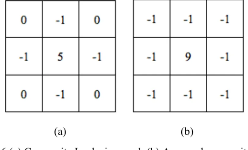
FIG. 2- 6 (A) COMPOSITE LAPLACIAN MASK (B) A SECOND COMPOSITE MASK. ...18

FIG. 2- 7 (A) ORIGINAL IMAGES. (B) RESULTS OF HISTOGRAM EQUALIZATION. ...20

FIG. 2- 8 THE PLOT OF PARABOLA EQUATION...22

FIG. 2- 9 MINKOWSKI ADDITION...24

FIG. 2- 10 MINKOWSKI SUBTRACTION...25

FIG. 2- 11 (A) SET A (B) STRUCTURING ELEMENT S AND ITS REFLECTION ! S" ...26

FIG. 2- 12 DILATION AND EROSION OF 1-D FUNCTION...28

FIG. 2- 14 MORPHOLOGICAL CONTRAST ENHANCEMENT FILTER...30

FIG. 2- 15 MORPHOLOGICAL CONTRAST ENHANCEMENT OF THE IMAGE IN FIG. 2- 13(A)...30

FIG. 2- 16 (A) SET ! A. (B) A WINDOW, ! W, AND THE LOCAL BACKGROUND OF ! X WITH RESPECT TO ! W, ! (W " X). (C) COMPLEMENT OF A. (D) EROSION OF A BY X. (E) EROSION OF ! Ac BY ! (W " X). (F) INTERSECTION OF (D) AND (E), SHOWING THE LOCATION OF THE ORIGIN OF ! X, AS DESIRED. ...34

FIG. 3- 1 OVERVIEW OF OUR PROPOSED METHOD...36

FIG. 3- 2 THREE TYPICAL KINDS OF HYPERBOLAS. FROM LEFT TO RIGHT ARE IRON、PVC AND PE...37

FIG. 3- 3 (A)-(C) THE IRON、PVC、PE PIPE IMAGES (D)-(F) THE BINARY IMAGE WITH THRESHOLD VALUE: 139、130、131，RANGE WITH [0,255] (G)-(I) THE HISTOGRAM. ....38

FIG. 3- 4 (A) LAPLACIAN OPERATOR (B) HISTOGRAM EQUALIZATION (C) PREWITT OPERATOR.39 FIG. 3- 5 (A) THE ORIGINAL IMAGE WITH TWO HYPERBOLA (B)THE BINARY IMAGE WITH THRESHOLD...41

FIG. 3- 6 BINARY IMAGES FOR DIFFERENCE HARD THRESHOLDING VALUE: 128,130,135, AND THIS RED...42

FIG. 3- 7 THESE STRUCTURING ELEMENTS OF MORPHOLOGICAL HIT-OR-MISS TRANSFORM...44

FIG. 3- 8 THE HYPERBOLA LOCATION MARKED WITH RED POINT...44

FIG. 3- 9 NO.1 IS THE POSITIVE POLE WAVE AND HIGH BRIGHTNESS HYPERBOLA; ...46

FIG. 3- 10 (A) A PHOTO HAS A ALARMING-BAND WHICH WAS CIRCLED BY RED CIRCLE AND...46

FIG. 3- 11 THE PARABOLA MODEL FLOWCHART...47

FIG. 4- 1 THE EXPERIMENT IMAGES OF GPR IMAGES. (A)-(D) IMAGE1-IMAGE4...49

FIG. 4- 2 THE HISTOGRAMS OF EXPERIMENT IMAGES. ...50

FIG. 4- 3 THE ILLUSTRATION OF THE HYPERBOLA LOCATION WITH RED COLOR...51

FIG. 4- 4 THE BINARY IMAGES WITH THE THRESHOLD VALUE 158, 140, 130, 156 ...52

FIG. 4- 5 THIS MORPHOLOGICAL STRUCTURES, THEIR SIZES ARE: ! 9 " 20, 15 "18...53

FIG. 4- 6 MORPHOLOGICAL HIT-OR-MISS TRANSFORM FIND THE POSSIBLE LOCATIONS OF HYPERBOLAS AND DETECT THE CORRECT HYPERBOLAS USING THE CONDITION WE PROPOSED. WE MARK THE LOCATIONS IN PROGRAMMING BY USING THE RED POINTS...54

FIG. 4- 7 THE PARABOLA MODEL...55

FIG. 4- 8 THE RESULTS OF USING THE PARABOLA MODEL...56

FIG. 4- 9 IMAGE1 THROUGH IMAGE4’S EACH HISTOGRAMS OF HYPERBOLAS. ...58

vii

FIG. 5- 1 THE DIFFERENT SITUATION OF HYPERBOLAS...66

FIG. 5- 2 THE ALTERED PARABOLA MODEL...67

FIG. 5- 3THE ILLUSTRATION OF THE PARABOLA MODEL CREATING AUTOMATICALLY (A) THE REAL IMAGE, ...68

FIG. 5- 4 THE PSEUDO-COLOR OF THE IMAGE1 ...69

FIG. 5- 5 THE EXAMPLE OF 3-D IMAGE OF IMAGE2 ...69

FIG. 5- 6 THE ILLUSTRATION OF 3-D MODEL OF THE PIPS IMAGES. ...70

LIST OF TABLES TABLE 4- 1 THE SIR-2 SYSTEM FUNCTION...48

TABLE 4- 2 THE U.S. GRP ANTENNA FUNCTION TABLE...49

TABLE 4- 3 THE RECORD OF THE SETTING AND THE DATA...58

CHAPTER 1

Introduction

1.1 Motivation

In recent decades, the GPR (Ground Penetrating Radar) is often used for exploring shallow stratums, the excavation, mineral resources, constructions, environmental pollution and ice sheets. No other ways can be better than it because it is easily used when we do the field exploration and it can cause high resolution of radar images. Due to the development of GPR equipments, more and more commercial products are entered the market. The GPR exploring ability has been improved with the amelioration of its hardware equipments, the way of exploration and the technique of information processing which considerably uses the Refseis model. Besides, it is widely utilized by construction industry and archaeologists with its increasingly emphasized technique of non-destructive exploration. It is also applied to: the exploration of unexploded bomb when doing military activities and before digging building sites, of discarded oil cans when doing environmental protection, of underground pipes before digging roads, of potholes when investigating the roadway of railways and highways, of the past and ancient graves when doing archaeological research, the put of underground rivers and find out the underground rivers.

In 50 years ago, someone had been brought up the idea of using the principle of radar wave reflection to explore the underground things such as pipes, hollows and depth of stratum (Melton,1937; Donaldson, 1953)[27][28]. It was not widely applied to explore the depth of polar excavation until 1960s (Cook, 1960)[29]. The results were applausive. The thesis will be focused on the image processing of exploring underground pipes (Lun-Dao Dong，1992:

2

information in Taiwan. Furthermore, there is no complete routine inspection, so we cannot carry out precautionary measures before finding out the problems. That is the main reason of resulting in pipe catastrophe. Besides, the pipes in the underground are densely distributed and it is dangerous to dig the roads with bad condition. In our country, most of public catastrophes are resulted from the uncertainty of pipe position. Therefore, investigating and judging pipe position fast can not only raise the constructors’ safety but also reduce time of ground routine affected by constructions and thus cause people inconvenient. Correct position and resolution of GPR images are two of solving the problem of underground pipes.

Concerning another benefit, it can help conserve the pipe information, pipe quality, solve and even prevent the problem of environmental pollution caused by underground pipes, and reduce the cost of road digging.

Aiming at the basic research of GPR, domestic experts precede a series of research

experiments, but there are not many ideas about the image processing of GPR section drawing. Concerning the pipe images, experts and researchers do not practically focus on the

recognition processing of pipe images to precede an in-depth study. There is still plenty of room for the research of non-metallic and metallic pipe images. Compared with metallic pipes, non-metallic pipes have higher distinguishing difficulty due to weaker radar waves. There are two kinds of non-metallic pipes, PE and PVC pipes, by which it causes highly similar images in GPR images, though PVC pipes have weaker signals than PE pipes. The motive of the thesis is to find out how to enhance effectively both types of images and find the correct location.

The thesis mainly aims at the GPR digital images of non-metallic underground pipes, but images are more difficult to be analyzed because Taiwan is formed with uneven geological layers. Now the research of scanned digital section of GPR depends on experts and

construction workers with great construction experiences or the complicated filter of software, so it brings problems of wrong results made by man-made mistake and an illusion resulted

from over filter processing. Because non- metallic pipes have weaker reflection of wave energy, the digital images transformed from the original data are weaker and not so clear as the images of metallic pipes. In [19][21], we know that the characteristics of pipe shapes in images are hyperbolas, and morphological is the best way of image processing to deal with shapes. For this reason, the main direction of the thesis is to combine the image strength with the morphological way to facilitate reliable recognition and assessments for experts and construction workers. The anticipated result will provide the correlative units with a reference of textual research distinguish non-metallic pipe image and assessments.

1.2 Background

Ground penetrating radar (GPR) is a non-destructive detection technique, it is relatively sensitive, fast and accurate than other general direct measure methods. GPR will not cause direct destruction in the objects which be examined. The developing history of Ground penetrating radar is among 1864~1995. Until 1970, Apollo 17 was implemented moon probing laboratory. And reach the middle 1980 time, the international GPR conference is established and thus began to have standards which specially uses the radar wave methods to detect underground. In 1980, The scholars began to make use of GPR to survey soil and Daniels et al. (1998) supposed that radar wave decayed in the soil layer has relative to conductivity in the soil itself. Davis & Annan(1989) measured the electricity of different materials, such as dielectric constant, conductivity, decay. Finally, in 1990, GPR was in it’s days which studies Geotechnical Engineering research, included the underground object’s study, the depth of the underground water, varying Soil Moisture Contents detection, the soil or the structure of soil layer’s study, the detection of the Earthdam of seepage hollow, etc.

4

the different dielectric of underground. Furthermore, the strongest signal which is not deep to detect is near the surface of ballast. In the process of detecting, it make signal unclear and mixed with a lot of the other signals that are all not come from the reflection of the surface of ballast due to noise, diffractive wave, and double reflection, and refracting wave. However, most of the situations can be improved by the conventional data treatment. Therefore, it is not discussed too much here. In brief, the reflection of GPR represents the relative depth of the surface of earth to surface of ballast so the actual position is viewed by a GPR digital image with the same system as image coordinate.

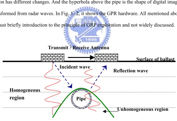
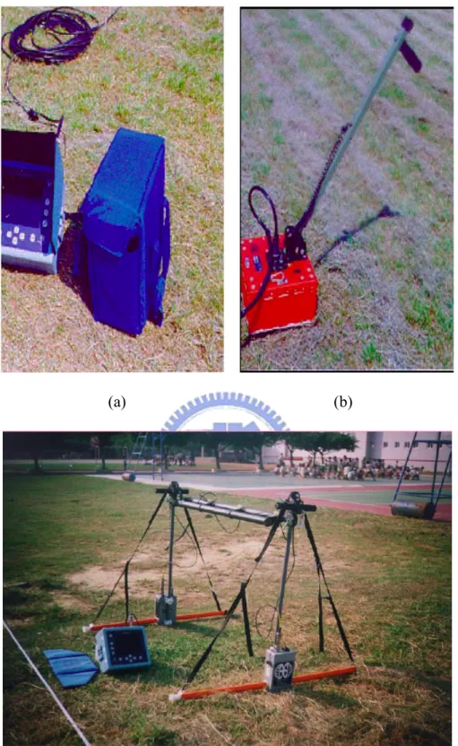
In Fig. 1- 1, it shows the investigated chart of Ground Penetrating Radar, indicating that the amplification of electromagnetic wave in homogeneous region and unhomogeneous region has different changes. And the hyperbola above the pipe is the shape of digital image transformed from radar waves. In Fig. 1- 2, it shows the GPR hardware. All mentioned above are just briefly introduction to the principle of GRP exploration and not widely discussed.

Fig. 1- 1 The illustration of the radar wave reflecting the underground pipe

Transmit / Receive Antenna

Incident wave Reflection wave Homogeneous

region

(a) (b)

(c)

Fig. 1- 2 GPR hardware photos. (a) The GPR system SIR-2 (b) The GPR antenna (400MHz) (c) The GPR antennas (16~80MHZ)

6

There are more relative studies of GPR, such as [1][2][3][5][9]. Majority studies have discuss for the GRP images, or make some explanation for some actual detection’s case, or direct GPR instruments to make differently efficient assessment and GPR’s detection methods to improve signal’s quality. But these studies have less to use image processing methods to direct the resolution of images and pipeline position to improve and deeply analyze them. The relative studies of above-mentioned have limited to the GPR hardware. So, if the studies want to continue going on, it must proceed with the professional instruments and GPR system’s additional software. The relative software are developed by the manufacturers of systems. And the format of GPR files which each manufacturer adopted has not been unified. So, the GPR data have not been extensively used.

In the part of image processing and GPR image processing, the brief chart of digital images are transformed from signal grasping which is explored by GPR system as shown in Fig. 1-3. In Fig. 1- 3(1), it is the objects of underground explored by GPR and stored as signals data. The chart is the figure of positive pole wave and negative pole wave.The quality in this stage is limited by equipments, human operation and environmental effects. It is what experts and construction workers are working for. In Fig. 1- 3(2), the signals of wave are translated to digital images through the procedure of traditional GPR information processing, like stacks, filter, shifting, etc. In the step, they are mostly processed by the hardware

provided by the GPR system, translating analogy signals to digital images. In this stage, many experts are proceeding the investigation of [4] and obtain better resolution of transformed images through improving the way of operating. In Fig. 1- 3(3), the software developed by system manufacturers provides a traditional way such as filter, shifting, and so on, to help experts or construction workers to proceed image processing. The advantages in the stage are not only to analyze the GPR image in the viewpoint of image processing with just the

problem of reading files but also to not be affected by hardware operation. However, it is limited by the way of image processing provided by manufacturers, though manufacturers

have developed adapter software. Thus, there is still a plenty of room for being independently discussed in details. We put Fig. 1- 3(1) and Fig. 1- 3(2) as the pre-processing, and Fig. 1- 3(3) as the post-processing.

Fig. 1- 3 The illustration of the GPR system translate the GPR signals to GPR digital image. (1) Probe and store the reflecting radar wave to signals (2) Using the stacks, sampling and other operators to translate the signals to Digital image (3) Image processing force on the digital image

The procedure of head process from (1) to (2) is investigated by most experts, and the main area for investigating the first kind of GPR researches as well. The thesis also aims at the (3) stage. Because the correlative thesis regarding the image of pipe GPR is seldom discussed in the stage, it is suitable to investigate the pipe image in the (3) stage in the viewpoint of image processing. Concerning correlative paper, it aims at GPR system which translates the signals to digital images as shown in Fig. 1- 3 in [20], and the penetrating radar section is processed by the way of image encoding. It then analyzes the internal cramp irons, cracks, holes and chips of concrete components through the thin method. In [23], it makes the characteristic of stratum clearer by strengthening GPR signals, raising the contrast of

lightness and darkness and being processed by gain filtering. It focuses on the GPR image of stratum, which is processed through filters, making the whole image clearer. Then, it links

(1) (2) (3) Hardware + Software Wave of Signals Only Software Digital image GPR system

8

of correlative paper mentioned above, it indicates that domestic and foreign scholars have done a lot of researches with diversification, while there are few researches which aims at pipes to investigate the image resolution and the exploration of pipe location.

Therefore, attempts would be made to raise the resolution of non-metallic pipe images, making the result fit human’s visual sense. Moreover, the written program can also be provided easily to experts or construction workers for usage without the limit of original system, so it is considerably reflex. The way of image processing is mainly referred to

morphological, spatial image enhancement, and segmentation. But due to few research related to GPR image processed through the way of image processing, it modifies traditional ways by means of traditional image processing as an assistant after a series of experimental discussion and GPR image analysis in the hope of improving the image effect and assisting the

information processing of images on the post-processing.

1.3 Organization of This Thesis

In this thesis, we propose to combine morphological hit-or-miss transform and the method of local image enhancement of the parabola model, which are the application for detecting hyperbolas and enhancing weak GPR images. The remainder of this thesis is organized as follows. In chaper1, first we introduce the probe theory of the GPR system, and then expound the probable problems when the signals translate to the images. Fig. 1- 4 show the procedure of our proposed method. In chaper2, we will survey spatial domain image enhancement methods, just about, the methods of Sobel, Prewitt, histogram equalization, morphological contrast enhancement, Laplacian, and the features of the histograms of the images. By using the thresholding histogram, we’ll separate the gray-levels to object point and background point. This can help us to separate the hyperbola and the rounding

background. Finally, we’ll survey the concept of morphological operations. In chapter 3, we will present our method which uses the global thresholding to transforms GPR images to

binary images for getting the shapes of objects of the GPR images. We’ll obtain the object points (the target pixels) and the background points by thresholding histogram. We designed two morphological structuring elements for hit-or-miss operator, According to these

structuring elements, we detect the probable location of hyperbolas and distinguish them. After detecting, we modify the “the parabola model” which is created by two parabola lines to become an area for doing “ local image enhancement”. By recovering the local areas to original images, we can distinguish clear hyperbolas. Our approach is just like to forecast the shape of hyperbola. The parabola model can enhance images easily more than enhance the full images.In chapter 4, we will experiment with different kinds of GPR images. Our

proposed method can efficiently enhance the hyperbolas in GPR images. Experimental results look “reasonable” to the human eye. Then, we will compare the performance of our method with other methods. In chapter 5, the conclusion and future work will be stated.

10

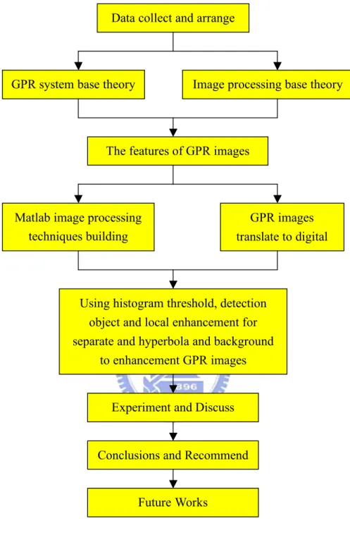
Fig. 1- 4 shows the procedure of our thesis. Data collect and arrange

Image processing base theory GPR system base theory

The features of GPR images

Matlab image processing techniques building

Future Works

Conclusions and Recommend Experiment and Discuss Using histogram threshold, detection

object and local enhancement for separate and hyperbola and background

to enhancement GPR images

GPR images translate to digital

CHAPTER 2

Previous Research

In the chapter we will introduce the background knowledge of our research. In section 2.1, we’ll describe some basic thresholding methods to separate background and object. In section 2.2, we will describe four basic and typical spatial image enhancement methods. More detail of these methods can be found in [10][12]. In section 2.3, we explain the equation of parabola, and how do it work. In section 2.4, we will discuss some basic concepts of mathematical morphology. They include binary morphology [14][15][16] and grayscale morphology [17][18].

2.1 Threshold

Because of its intuitive properties and simplicity of implementation, image thresholding enjoys a central position in application s of image segmentation. Suppose that the gray-level histogram shown in Fig. 2- 1 (a) corresponds to an image, f(x,y) , composed of light objects on a dark background, in such a way that object and background pixels have gray levels grouped into two dominant modes. One obvious way to extract the objects from the background is to select a threshold T that separated these modes. Then any point (x,y) for which f(x,y) > T is called an object point; otherwise, the point is called a background point.

12

(a) (b)

Fig. 2- 1 (a) Gray-level histograms that can be partitioned by (a) A single threshold. And (b) Multiple threshold.

Fig. 2- 1(b) shows a slightly more general case of this approach, where three dominant modes characterize the image histogram, for example, there two light objects on a dark background. Here, multilevel thresholding classifies a point (x,y) as belonging to one object class if

!

T1< f (x, y) " T2, to the other object class if

!

f (x, y) > T2, and to the background if

!

f (x, y) " T1.

Based on the preceding discussion, thresholding may be viewed as an operation that involves tests against a function T of the form

!

T = T[x, y, p(x, y), f (x, y)] (2- 1) where f(x,y) is the gray level of point (x,y) and p(x,y) denotes some local property of this point– for example, the average gray level of a neighborhood centered on (x,y). A thresholded image g(x,y) is defined as

! g(x, y) = 1 if f (x, y) > T 0 if f (x, y) " T # $ % (2- 2)

Thus, pixels labeled 1 correspond to objects points whereas pixels labeled 0 correspond to background points.

Where T depends only on f(x, y) (that is, only on gray-level values) the threshold is called global. If T depends on both f(x, y) and p(x,y), the threshold is called local. If, in addition, T depends on the spatial coordinates x and y, the threshold is called dynamic or adaptive.

T

!

T

!

2.2 Spatial Image Enhancement Methods

In general, the implementation for filtering an

!

M " N image with a weighted averaging

filter of size

!

m " n (m and n odd) is given by:

! g(x, y) = w(s,t) f (x + s, y + t) t="b b

#

#

#

#

Fig. 2- 2 denotes image points in a

!

3 " 3 region. For example, the center point,

!

z5,

denotes f(x,y),

!

z1 denotes f(x-1,y-1), and so on. In following paragraph, we will introduce

two useful methods.

Fig. 2- 2 A

!

3 " 3 region of an image (the

!

z's are gray-level values) used to compute the gradient at point labeled

!

z5

2.2.1 Prewitt and Sobel Operators

For a function

!

f (x, y) , the gradient of f at coordinate (x,y) is defined as the two-dimensional column vector

14 ! "f = Gx G_y # $ % & ' ( = )f )x )f )y # $ % % % % & ' ( ( ( ( (2- 4)

It is well known from vector analysis that the gradient vector is in the direction of maximum rate of change of f at coordinates (x,y). The magnitude of this vector is given by

! "f = mag("f) = Gx 2 + Gy 2

[

]

This quantity gives the maximum rate of increase of f(x,y) per unit distance iin the direction of

!

"f.

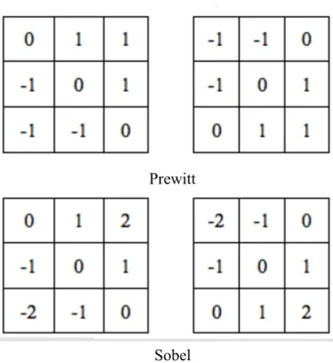
Prewitt

Sobel

Fig. 2- 3 Prewitt and Sobel masks for detecting vertical and horizontal edges

The components of the gradient vector itself are linear operators, but the magnitude of this vector obviously is not because of the squaring and square root operations. However, The computational burden of implementing Eq.(2-5) over an entire image is not trivial, and it is common practice to approximate the magnitude of the gradient by using absolute values instead of squares and square roots.

!

"f # Gx + Gy (2- 6)

This equation is simpler to compute and it still preserves relative changes in gray levels, but the isotropic feature property is lost in general. However, the most popular masks used to approximate the gradient give the same result only for vertical and horizontal edges and thus the isotropic properties of the gradient are preserved only for multiples of

!

90°. These results are independent of whether Eq.(2-4) is used, so nothing of significance is lost in using the simpler of the two equations.

Fig. 2- 4 Prewitt and Sobel masks for detecting diagonal edges.

Finally, the Prewitt and Sobel operators are aomong the most used in practice for computing digital gradients. Masks in Fig. 2- 3 are used for detecting vertical and horizontal edge while masks in Fig. 2- 4 are used for detecting diagonal edges. The Prewitt masks are simpler to implement than the Sobel masks, but the latter have slightly superior

noise-suppression characteristics.

Prewitt

16

2.2.2 Laplacian

The approach basically consists of defining a discrete formulation of the second-order derivative and then constructing a filter mask based on that formulation. It can be shown (Rosenfeld and Kak [1982]) hat the simplest isotropic derivate operator is the Laplacian, which, for a function (image)

!

f (x, y) of two variables, is defined as

(2- 7)

Because derivatives of any order are linear operations, the Laplacian is a linear operator. In order to be useful for digital image processing, this equation needs to be expressed in discrete form. There are several ways to define a digital Laplacian using neighborhood. Taking into account that we now have two variables, we use the following notation for the partial second-order derivative in the x-direction:

!

"2f

"2x2 = f (x + 1, y) + f (x #1, y) # 2 f (x, y) (2- 8) and, similarly in the y-direction:

!

"2f

"2y2 = f (x, y + 1) + f (x, y #1) # 2 f (x, y) (2- 9) The digital implementation of the two-dimensional Laplacian in Eq.(2-7) is obtained by summing these two components:

!

"2f = f (x + 1, y) + f (x, y + 1) + f (x #1, y) + f (x, y #1)

_[

_]

The equation can be implemented using the mask shown in (Fig. 2- 5.) For a 3×3 region, one of the two forms encountered most frequently in practice is

!

"2f = (z2+ z4+ z6+ z8) # 4z5 (2- 11)

where the z’s are defined inFig. 2- 2. A digital approximation in clouding the diagonal neighbors is given by

!

"2f = (z1+ z2+ z3+ z4+ z6+ z7+ z8+ z9) # 8z5 (2- 12)

This two equations can be implemented using the mask shown in Fig. 2- 5(a) and (b). We noted from these masks that the implementations of Eq.(2-10) and Eq.(2-11) are isotropic for rotation increments of

!

90o and

!

45o, respectively. The other two masks show in Fig. 2- ! "2f =# 2_f #x2 + #2f #y2

(a)

5(c)-(d) also are used frequently in practiece. They are based on a definition of the Laplacian that is the negative of the one we used here. The difference is sign must be kept in mind when combining (by addition or subtraction) a Laplacian-filter image with another image.

Because the Laplacian is a derivative operator, its use highlights gray-level

discontinuities in an image and deemphasizes regions with slowly varying gray levels. This will tend to produce images that have grayish edge lines and other discontinuities all superimposed on a dark, featureless background. Background features can be “recovered” while still preserving the sharpening effect of the Laplacian operation simply by adding the original and Laplacian images. It is important to keep in min which definition of the

Laplacian is used. Thus, the basic way in which we use the Laplacian for image enhancement is as follows:

!

g(x, y) =

f (x, y) " #2

f (x, y) if the center coefficient of the Laplacian mask is negative

f (x, y) + #2f (x, y) if the center coefficient of the Laplacian mask is positive $ % & & ' & & (2- 13)

Fig. 2- 5 Filter masks used to implement the digital Laplacian The coefficients of the single mask are easily obtained by substituting Eq.(2-12) for

"2f (x, y) in the first line of Eq.(2-13):

(a) (b)

18 !

g(x, y) = f (x, y) " f (x + 1, y) + f (x, y + 1) + f (x "1, y) + f (x, y "1)

_[

_]

= 5 f (x, y) " f (x + 1, y) + f (x, y + 1) + f (x "1, y) + f (x, y "1)

_[

_]

(a) (b)

Fig. 2- 6 (a) Composite Laplacian mask (b) A second composite mask.

2.2.3 Histogram Equalization

The probability of occurrence of gray level

! rkin an image is approximated by ! p_r(r_k) = nk n k = 0,1,2,K,L "1 (2- 15) where, n is the total number of pixels in the image,

!

nk is the number of pixels that have gray

level

!

rk, and L is the total number of possible gray levels in the image. The discrete version

of the transformation function is

! sk = T(rk) = pr(rj) j= 0 k

"

"

Thus, a processed (output) image is obtained by mapping each pixel with level

!

rk in the

input image into a corresponding pixel with level

!

sk in the output image via Eq.(2-15). A

plot

!

pr(rk)of versus

!

Eq.(2-15) is called histogram equalization or histogram linearization. On the other hand, the inverse transformation from s back to r is denoted by

!

r_k= T"1(s_k) k = 0,1,2,K,L "1 (2- 17)

Only if none of the levels, !

rk,k = 0,1,2,K,L "1, are missing from the input image. In addition

to producing gray levels that have this tendency, the method just derived has the additional advantage that it is fully “automatic.” In other words, given an image, the process of histogram equalization consists simply of implementing Eq.(2-16), which is based on information that can be extracted directly from the given image, without the need for further parameter specifications.

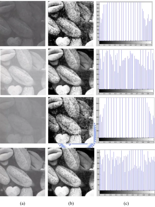
Fig. 2- 7(a) shows the four basic image types: dark, light, low contrast, high contrast, and Fig. 2- 7(b) shows the result of performing histogram equalization on each of these images. The first three results (top to bottom) show significant improvement. As expected, histogram equalization didn’t produce a significant visual difference in the fourth image because the histogram of this image already spans the full spectrum of the gray scale. The histograms of the equalized images are shown in Fig. 2- 7(c). All these histograms are different, the histogram equalized images themselves are visually very similar. This isn’t unexpected because the difference between the images in the left column is simply one of contrast, not of content. In other words, since the images have the same content, the increase in contrast resulting from histogram equalization was enough to render any gray-level differences in the resulting images visually indistinguishable. Given the significant contrast differences of the images in the left column, this example illustrates the power of histogram equalization as an adaptive enhancement tool.

20

(a) (b) (c)

Fig. 2- 7 (a) Original images. (b) Results of histogram equalization. (c) Corresponding histograms

2.3 The Equation of Parabola

The equation of a Parabola is also called Cartesian equation too. The parabola’s equation in standard polynomial form is denoted by:

!

y = ax2+ bx + c (2- 18)

Fig. 2- 8 shows a plot of equation of parabola. In Eq.(2-18), x is called the independent variable (the horizontal axis on the graph) and y is called the dependent variable (the vertical axis), and a, b and c called parameters. Although it is also possible to choose values for a, b and c arbitrarily, for any one particular parabola their values will not change. A new set of values for a, b and/or c will result in a different parabola. The graph of

!

y = ax2+ bx + ctakes

the shape of the cross-section of a bowl, opening either upwards or downwards. The lowest point when it opens upwards (or the highest point when it opens downwards) is called the vertex. All parabolas with the above equation will cross the y-axis somewhere, but need not necessarily cross the x-axis Here y is a function of (i.e. depends on) x, written y = f(x) in general, so here we can write

!

f (x) = ax2

+ bx + c. In this case, f(x) is called the quadratic

function. The quadratic function has important applications in the mathematical analysis of topics in, amongst others, science, technology and business studies – in particular in cases where there is a square-law relationship between two sets of variables.

The equation of parabola still have the another types: Standard Form Equation:

! (x " h)2 = 4c(y " k) # y = 1 4c (x " h) 2 + k # y = m (x " h)2+ k (2- 19)

where, some basic definitions are given by: Vertex:

!

(h,k) ,

Axis of symmetry: x = h, Focus: h = k + c,

22 Opens: up if c > 0 / down if c < 0

For exampleL

· the cross-sectional shape of a car's headlamp reflector is parabolic, and

· the aerodynamic drag of a moving vehicle is proportional to its velocity squared.

2.4 Mathematical Morphology

Mathematical morphology is closely related to integral geometry (show [11]) and it quantifies many aspects of the geometrical structure of images in a way that agree with human intuition and perception. Mathematical morphology has been also a valuable tool in many computer vision applications, especially in the area of automated visual inspection.

Morphological expressions are defined as the combinations of basic operations known as erosions and dilations. The morphological approach analyzes an image in terms of some predetermined geometric shape templates known as elemental structuring elements. The manner in which the structuring elements can be embedded into the original shape using a specific sequence of operations leads eventually to shape classification and/or discrimination.

In the following sections, we first introduce the fundamental morphological operations upon which the entire subsequent development depends. We then discuss the extensions of binary morphological operations to the gray-value morphological operations.

There are two types of fundamental operations in mathematical: dilations and erosions, each associated with a structuring element. These two types of operations are both based on the Minkowski operations will be discussed below.

2.4.1 Morphological Operations

Some basic definitions:

E: the n-dimensional Euclidean space

!

P(E) : The power set of E.

!

A_b : The set of translation of A by b given by a + b | a " A

{

}

S": The reflected set of A with respect to the orgin given by #a | a $ A

{

}

24 b!B

B={(4,1),(5,1),(5,2)} A ! B

Minkowski Addition

Let A and B be two sets in P(E). The Minkowski addition of A and B, denoted A⊕B, is defined as

A ⊕ B = { a + b | a ! A and b ! B }. (2- 20)

In terms of translation, the Minkowski addition of A and B can also be written as

A ⊕ B = ∪Ab. (2- 21)

Thus A ⊕ B is constructed by translating A by each element of B and then taking the union of all the resulting translates

For example, let A be the unit disk centered at (2,2) and let B={(4,1), (5,1), (5,2)}. Then A ⊕ B is the union of the sets

!

A_(3,1), A_(5,1), and

!

A_(5,2). A, B, and A ⊕ B are depicted in Fig. 2-

9

Minkowski Subtraction

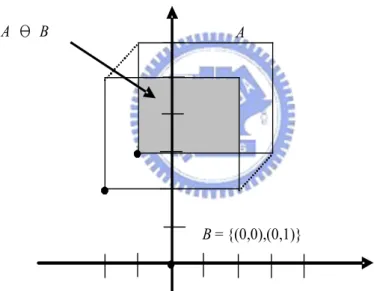
Let A and B be two sets in P(E). The Minkowski subtraction of B from A, written as A0B, is defined by A 0 B = ! A " b = A_b b #B$

I

I

In this operation, A is translated by the reflection of B and then the intersection is taken. For example, consider the 4 by 3 rectangle A. Let B = {(0,0),(1,1)}. Then A0B is the intersection of the translates

!

A_"(0,0) and

!

A_"(1,1). That is, A0B is the the 3 by 2 rectangle depicted in Fig. 2- 10.

Fig. 2- 10 Minkowski subtraction

2.4.2 Structuring Element

A structuring element is also a set in P(E), however, it is usually chosen to have simple shape and small size. The structuring element can be viewed as a convolution mask.

Therefore, dilations and erosions are analogous to the convolution processes.

Dilation

B = {(0,0),(0,1)}

26

The set Ds( A) is called the dilated set of A by the structuring element S. Geometrical meaning: Ds(A)={x$E|Sx #A"!}.

Erosion

The erosion Es( A) with a structuring element S is a unary operation on P(E) defined by A

A

Es( )= 0S. (2- 24) The set Es( A) is called the eroded set of A by the structuring element S.

Geometrical meaning: Es(A)={x"E|S_x ! A}.

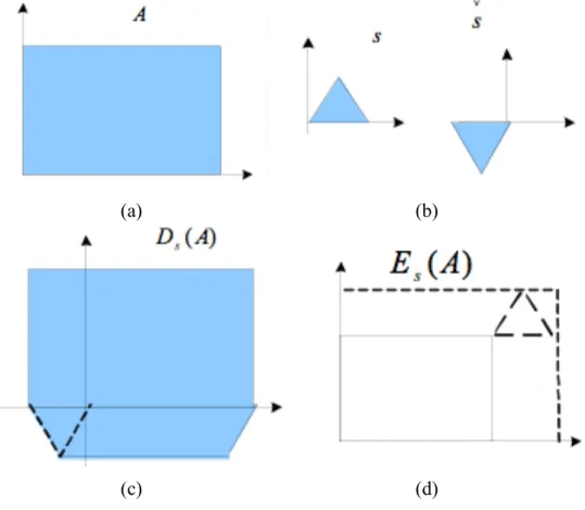
For example, consider a set

!

A(Fig. 2- 11(a)) and a structuring element

!

S (Fig. 2- 11(b)). Dilating the set

!

A by the structuring element

!

S has the effect of “expanding” the set. (see Fig. 2- 11(c)). Erosion has the effect of “shrinking” the set (see Fig. 2- 11(d)).

Fig. 2- 11 (a) Set A (b) Structuring element S and its reflection

!

S" (c) Dilation of A by S (d) Erosion of A by S

(a) (b)

2.4.3. Extensions to Gray-scale Morphology

In this section we extend to gray-level images the basic operations, dilation and erosion. Throughout the discussions that follow, we deal with digital image functions of the

forms f x y( , )andb x y( , ), where f x y( , )is the gray-scale image andb x y( , )is a structuring element, itself an image function.

Dilation

Dilation

!

D( f ,b) of the gray-scale image

! f by structuring element ! b, denoted as ! f " b, is defined as ! ( f " b)(s,t) = max (x,y )

{

}

Where Df and D are the domain of b f and b, respectively. The dilation methodology is

illustrated in Fig. 2- 12. Because the dilation is based on choosing the maximum value of

!

f + b in a neighborhood defined by the shape of the structuring element, the general effect of performing dilation on a gray-scale image is two-fold: (1) if all the values of the structuring element are positive, the output image tends to be brighter than the input; and (2) dark details either are reduced or eliminated, depending on how their values and shapes relate to the structuring element used for dilation.

Erosion

The erosion

!

D( f ,b) of the gray-scale image

! f by structuring element ! b, denoted as f0b, is defined as ! ( f0 ! b)(s,t) = min (x,y )

{

}

Fig. 2- 12(e) shows the result of eroding the function of Fig. 2- 12(b) by the structuring element of Fig. 2- 12(a). As Eq.(2-26) indicates, erosion is based on choosing the

28

elements of the structuring element are positive, the output is tends to be darker than the input image; and (2) the effect of bright details in the input image that are smaller in “area” than the structuring element is reduced, with the degree of reduction being determined by the

gray-scale values surrounding the bright detail and by shape and amplitude values of the structuring element itself.

Fig. 2- 12 Dilation and erosion of 1-D function

For example, Fig. 2- 13(a) shows

!

172 "112 gray-scale image, and Fig. 2- 13(b) shows the result of dilating the image with a “flap” structuring element with size

!

5 " 5 pixels. Based on the preceding discussion, dilation is expected to produce an image that is brighter than the original image and in which small, dark detail have been reduced or eliminated. These effects clearly are visible in Fig. 2- 13(b). Not only does the image appear brighter than the original,

) (s₂ f ) (s₁ f f t b t ) ( ) (s₁ b s₁ x f + ! f(s2)+b(s2 !x) t (a) (c) (b) t ) , ( bf D (d) ) , ( bf E t (e) 1/2

but the size of dark features has been reduced. Fig. 2- 13(c) shows the result of eroding the original image.Note the opposite effect to dilation. The eroded image is darker, and the sizes of small, bright features are reduced.

Fig. 2- 13 Dilation and erosion of image in Fig. 2- 13(a). (a) Original image; (b) Result of dilation; (c) Result of erosion.

2.4.4 Morphological Contrast Enhancement

In addition to the operations discussed earlier in connection with the removal of small dark and bright artifacts, dilation and erosion often are used to compute the morphological contrast enhancement of an image, denoted g:

f b f

g =( " )!( 0b). (2- 27) Fig. 2- 14shows the actions of morphological contrast enhancement. Fig. 2- 15 shows the result of computing the morphological contrast enhancement of the image shown in Fig. 2- 13(a). As expected, the morphological contrast enhancement highlights sharp gray-scale transitions in the input image. The morphological contrast enhancement is sensitive to the shape of the chosen structuring element. As such, the adaptive structuring element has been

30 important filter for our proposed method.

Fig. 2- 14 Morphological contrast enhancement filter

Fig. 2- 15 Morphological contrast enhancement of the image in Fig. 2- 13(a) (a)

f

2.4.5 Morphological Hit-or-Miss Transform

The morphological hit-or-miss transform is a basic tool for shape detection. We introduce this concept with the aid of Fig. 2- 16 which shows a set

!

Aconsisting of there shapes (subsets), denoted

!

X,Y and

!

Z. The shading in Fig. 2- 16(a) through Fig. 2- 16(c) indicates the original sets, whereas the shading in Fig. 2- 16 (d) and (e) indicates the result of morphological operations. The objective is to find the location of one of the shapes, say,

!

X. Let the origin of each shape be located at its center of gravity. Let

!

X be enclosed by a small window, W. The local background of

!

X with respect to W is defined as the set difference

!

(W " X), as shown in Fig. 2- 16 (b). Fig. 2- 16 (c) shows the complement of

!

A, which is needed later. Fig. 2- 16 (d) shows the erosion of

!

A by

!

X (the dashed lines are included for reference). Recall that the erosion of

!

A by X is the set of locations of the origin of

!

X, such that

!

X is completely contained in A. Interpreted another way, A 0

!

X may be viewed geometrically as the set of all locations of the origin of X at which X found a match (hit) in A. Keep in mind that in Fig. 2- 16

!

A consists only of the three disjoint sets

!

X,Y and

!

Z. Fig. 2- 16 (e) shows the erosion of the complement of

!

A by the local background set

!

(W " X). The outer shaded region in Fig. 2- 16(e) is part of the erosion. We note from Fig. 2- 16 (d) and (e) that the set of locations for which exactly fits inside

! A is the intersection of the erosion of ! A by !

X and the erosion of Ac by

!

(W " X)as shown in Fig. 2- 16 (f). This intersection is precisely the location sought. In other words, if

!

B denotes the set composed of

!

X and its background, the match (or set of matches) of B in

!

A, denoted A○B, is

A ○ B = (A 0 X) ∩ [Ac _{0 (W – X )], (2- 28)}

We can generalize the notation somewhat by letting B = (B1, B2), where B1 is the set formed from elements of B associated with an object an B2 is the set of elements of B associated with the corresponding background. From the preceding discussion, B1 = X and B2 = (W " X).

＊

32 A ○ B = (A 0B1) ∩ (Ac _{0 B}

2). (2- 29)

Thus, set

!

A B contains all the (origin) points at which, simultaneously, B1 found a match

(“hit”) in

!

A and B2 found a match in Ac. There are two definition will be set, the first is the

difference of two sets

! A and B, denoted ! A " B, is defined as ! A " B = w | w # A,w $ B

{

}

complementation and reflection, is defined as

!

(A0

!

B)c

= Ac " B# (2- 31) By using the definition of set the differences given in Eq. (2-30) and the dual relationship between erosion and dilation given in Eq.(2-31), we can write Eq.(2-29) as

A ○ B = (A0B1 ) – (A ⊕

!

B"2). (2- 32)

The reason for using a structuring element B1 associated with objects and an element B2

associated with the background is based on the aseemption that two or more objects are distinct only if they form disjoint (disconnected) sets. This is guaranteed by requiring that each object have at least a one-pixel-thick background around it. In some applications, we may be interested in detecting certain patterns(combinations) of 1’s and 0’s within a set, in which case a background is not required. In such an instance, morphological hit-or-miss transform reduces to simple erosion. As indicated previously, erosion is still a set of matches, bur without the additional requirement of a background match for detecting individual

objects.

＊

Y

X

A = X∪Y∪Z

Origin

34 Fig. 2- 16 (a) Set

!

A. (b) A window,

!

W, and the local background of

!

X with respect to

!

W,

!

(W " X). (c) Complement of A. (d) Erosion of A by X. (e) Erosion of

!

Ac by

!

(W " X). (f) Intersection of (d) and (e), showing the location of the origin of

!

X, as desired.

(A Θ X)

∩

(A

Θ (W – X))

CHAPTER 3

The Proposed Method

3-1 The System Structure

In this chapter we propose a method, which combines morphological hit-or-miss transform and local thresholding. Our objective in this thesis is to propose a method for improving the resolution of a GPR Image. Thewave energies reflect non-metallic pipes and are weaker than reflected by metallic pipes when we grasp images by using Penetrating Radar Equipments, thus these images are transformed worse than pipe images.

Aiming at this kind of images, we propose a parabola-shape partial image segmentation way through the comparison of other image enhancement methods. The GPR images we adopt in this thesis are all obtained by SIR-2 GPR system experiments. The flowchart is as follows:

36

Fig. 3- 1 Overview of our proposed method GPR Image: *.dzt

Grey-value Image: 8-bit

Binary Image: Threshold

Detect object:

Morphological Hit-or-Miss Transform Cluster

Object Situation

Compare object’s size

Create Parabola Model

Double Refection Wave Have Noises

Local Enhancement Image

Recover Original Image Filter

In this section, we first introduce properties GPR images. Generally, there are two kinds of underground pipes. One is metal series, including iron pipes in general, which can result in clear hyperbola images when images are transformed because they can reflect higher energy waves. The other is non-metallic series, including plastic pipes made of PVC and PE

materials, which result in more easily weak hyperbola images when images are transformed because they reflect weaker waves than metal pipes. Fig. 3- 2 shows three typical hyperbolas, the signal of IRON pipe is stronger than those of PVC and PE pipes. In the thesis we will focus on the enhancement of PVC and PE pipe images. Because the pipe images obtained by experiments are in shapes of hyperbolas, in the thesis we will attempt to develop an image processing method based on this point.

Fig. 3- 2 Three typical kinds of hyperbolas. From left to right are IRON、PVC and PE

First of all, we try to explain hyperbolas as shown in Fig. 3- 2. From the Fig. 3- 3 it may note that only IRON pipes can grasp complete hyperbolas; otherwise, the hyperbolas caused by PVC and PE pipes have been broken. When the threshold value is lowered, the hyperbolic objectcan’t be separated from background, the gray values ofnon-metallic pipe (PVC,PE) image are very similar with background’s. In Fig. 3- 3 (h) we can find that PVE and PE pipes with low contrast have histograms that will be narrow and will be centered toward the middle of the gray scale. IRON pipe images in general are clearer, so it is easily to know the position of pipes when experts compare with them with others. While PVE and PE pipes are much more easily affected by image surrounded and noise, it may cause us investigate the wrong

38 (a) (b) (c) (d) (e) (f) (g) (h) (i)

Fig. 3- 3 (a)-(c) The IRON、PVC、PE PIPE images (d)-(f) The binary image with threshold value: 139、130、131，range with [0,255] (g)-(i) The histogram.

Traditionally, image enhancement methods are worked in spatial domain. We have discussed five main methods for PVC and PE GPR images, which are Prewitt, Sobel,

Laplacian, Morphological contrast enhancement, and Histogram Equalization. Fig. 3- 4 shows the effect of different image processing. First, we mask the positive hyperbola with the red circles in Fig. 3- 4(b), where we can see the enhanced hyperbola is stronger than the original one. From these pictures it is apparent that IRON has well effect for this methods, on the another hand, in Fig. 3- 4 (a) and (e)strengthens little the effect and thus makes PVC and PE images clearer, but the positive hyperbola still is similar with the background in gray value; in Fig. 3- 4 (c) through (d) PVC and PE pipe images are weak when using Prewitt and Sobel. In Fig. 3- 4(e), Morphological contrast enhancement enhances the PE pipes well, the more

significant effect than others. However, it is still weak in PVC pipes. Above methods are not still sturdy. Last of all, it has the remarkable effect when using Histogram equalization (Fig. 3- 4(b)). In these ways, PE pipes have good effects. However, when the whole image is strengthened, the noise is strengthened at the same time in the GPR images. If we don’t denoise it well, weakened hyperbola may easily be eliminated. Therefore, enhancing the whole image does not necessarily optimize the image.

Finally, the GPR image’s histogram shows that it is the low contrast image and shows the GPR image belongs unimodal histogram. On PE and PVC pipes, the hyperbolas are close to background in gray value, it is a question to separate them that we’ll discuss.

(a) (b)

(c) (d)

(e) (f)

40

Then we use the same procedure to process another image. First of all, as in Fig. 3- 5(a), two places which have been circled are hyperbolas. The same as in Fig. 3- 5(c), two hyperbola which have been marked with red lines. This is a high contrast and weak image and the pixels value is also similar to background, we found that we cannot separate hyperbolas from

background by using threshold: 136(Fig. 3- 5). And it is still the same situation after using other spatial domain image enhancement method. We hope get the clear hyperbola which has the more difference from background, that help experts easy to distinguish it. Above image enhancement methods can’t satisfy us. In Fig. 3- 4(e), we found the result of morphological contrast enhancement method is fairly good than other traditional methods. Analysis these two images, Fig. 3- 4 belongs to unimodal histogram, but gray levels of histogram of Fig. 3- 5 distributes averagely, object edge is not clear and the image is high contrast, too. Under the condition of Fig. 3- 4, using histogram equalization can produce significant and desirable effect. If using the other 4 methods stated above, image in Fig. 3- 4 can produce the results better than that in Fig. 3- 4, but they still can be improved. This is because that the histogram of Fig. 3- 4 is narrow and the histogram of Fig. 3- 4 is wide. So using histogram equalization can’t get fairly good effect. So, in Fig. 3- 4 can obtain better result than in Fig. 3- 5 using other methods stated above. It is because it has clearer edge in Fig. 3- 4. Meanwhile, Fig. 3- 5 actually cannot achieve desirable result adequately from either method above. In a weakened image, we usually face the problems of hyperbola being similar to the background in gray value, and mistrial problem due to noise image. We introduce hyperbola model to produce regional area to process hyperbolic object, in order to help the experts to distinguish images and solve the above problems. Thus, if we can get the local histogram that only formed by the hyperbola pixels, we don’t care pixels of the background.

(a) (b)

(c) (d)

(e) (f)

(g) (h)

Fig. 3- 5 (a) The original image with two hyperbola (b)The binary image with threshold value:136 (c) Laplacian operator (d) Histogram equalization (e) Prewitt operator

42

3-2 Image Processing Technique

The images in this thesis are gray-value images of 8-bit. Gray value is the only reference. Since the hyperbola always looks similar to the surrounding information, it is not easy to generalize, from the histogram’s distribution, a suitable way for manual threshold value determination. Using the other methods to determine the threshold value[8] can’t be

appropriately applied to this thesis. Hence, we decide the threshold value by manually setting it, then processed hard thresholding on the image, in order to get the primary shape of the image. We found that the threshold values being set are mostly range at about 130 gray levels, which is a fairly good reference value for us to do the trimming , minimizing the potential adjustment range. That will be helpful in automatic threshold value determination. Finally, we still have to decide whether the term to choose the threshold value can retain the hyperbola. Fig. 3- 6 shows that threshold value range at about 128-135 only. When threshold value is 128, the PVC and PE connected with each other ; when the threshold value is 130, we can get the hyperbolas; when the threshold value is 135, the PVC hyperbolas disappear.

(a) (b)

(c)

Fig. 3- 6 Binary images for difference hard thresholding value: 128,130,135, and this red circles mean invisible object and the red rectangle mean the object location.

3-2-2 Morphological Hit-or-Miss Transform

Traditionally, if hoping to use morphological hit-or-miss transform to find the correct object location, the object must match the structured element totally. But due to the fact that the shapes of hyperbola we’re looking for are not alike totally. We provide two parameters to hit or miss percentage, namely, hit percentage and miss percentage, respectively. And use the corresponding threshold value to trim the proportion of the threshold value and to get the object location of appropriate hyperbola feature. We observe certain amount of the hyperbola, and find out the most frequently exist the hyperbolic radian, in order to use them in designing 2 structured elements of morphological hit-or-miss transform. In Fig. 3- 7, the subset of blue number (no.1) is the hit structuring element and the subset of red number (no.2) is the miss structuring element, finally, the subset of white number (no.0) is don’t care.

In the GPR images, we can regard hyperbola as parabola and same as our structuring elements. The parabola equation is y =m(x! p)2 +q, m is the slope that is used to change the curve rate. If m is big, the parabola shape is steep, on the other hand, if m is smaller, the parabola shape is flat. According to different GPR images, we can also change the structuring element size. In Fig. 3- 8, we can see how the structuring element matches the hyperbola. The hyperbolas always have peak, this shape is the hyperbola feature. According to the feature, we can find the locations of hyperbolas.

44

(a) (b)

(c) (d)

Fig. 3- 7 These structuring elements of morphological hit-or-miss transform

3-2-3 Object Detection

In this section, we’ll discuss how to remove the wrong object. First, we introduce GPR images formation theory。Illustrating at Fig. 3- 9，when the radar wave hit the pipes, the instrument will get the reflections of the signals, thus, recording the signal waves. A complete wave will have both positive (₁₈₀o_{) and negative (!180}o_{) poles. Hence, when the waves}

transform to GPR gray-value images, the both positive and negative poles, respectively, obtain an corresponding images. And this pair of hyperbola is the pipe image feature, one is high brightness hyperbola, another is low brightness hyperbola. When the morphological hit-or-miss transform find the wrong object location, we classify them to two types: (1) noise: even though some noises match the morphological hit-or-miss transform structuring element, but their shapes or size will very different from the correct hyperbola. We measure the rectangle size and the areas for all objects that were found out by morphological hit-or-miss transform. (2) similar hyperbola: there are two common conditions that usually exist, one is , the pipes are beneath the Alarming-band, while the Alarming-band is shallowly beneath the surface of ballast; while the other one, when the double reflection happens on the wave, there would occur one or more similar hyperbola images right under its hyperbola. Fig. 3- 10 (a) shows that a photo has a Alarming-band and a pipe, we let the red double-arrowhead mean the pipe direction. In Fig. 3- 10(b) shows that the feature image of the surface of ballast is two almost straight and energetic straps. Since pipes are not necessarily buried very close to the surface of ballast, when there occur the similar hyperbolic image, we’ll consider it as alarming-band, and determine that it is not the pipe. In Fig. 3- 10(c) there are two similar hyperbola images under the correct hyperbola, so we also regard them as the wrong objects. This similar hyperbola is the double reflection waves.

46

Fig. 3- 9 No.1 is the positive pole wave and high brightness hyperbola; No.2 is the negative pole wave and the low brightness hyperbola

(a)

(b) (c)

Fig. 3- 10 (a) A photo has a alarming-band which was circled by red circle and has a pipe was marked by a red line that show the piped direction (b) A alarming-band is similarly to hyperbola under the ballast surface (c) There are two double reflection waves under the correct hyperbola

wave A pipe 1 2 (1) (2) Alarming-band pipe Surface of ballast