半競爭風險資料受限於左截切的半母數推論

國 立 交 通 大 學

統計研究所

碩士論文

半競爭風險資料受限於左截切的半母數推論

Semi-parametric Inference for

Semi-competing Risks Data subject to

Left Truncation

研究生： 林怡君

指導教授：王維菁 教授

半競爭風險資料受限於左截切的半母數推論

Semi-parametric Inference for

Semi-competing Risks Data subject to

Left Truncation

研 究 生：林怡君 Student：Yichun Lin

指導教授：王維菁 Advisor：Weijing Wang

國 立 交 通 大 學

統計學研究所

碩 士 論 文

A Thesis

Submitted to Institute of Statistics College of Science National Chiao Tung University

in Partial Fulfillment of the Requirements for the Degree of Master

in Statistics

June 2007

Hsinchu, Taiwan, Republic of China

半競爭風險資料受限於左截切的半母數推論

研究生：林怡君 指導教授：王維菁 教授

國立交通大學統計研究所碩士班

摘 要

本論文考慮以半母數推論方法估計在半競爭風險資料受限於左截切下的關連性。半 競爭風險是多重事件發生的過程。以糖尿病的例子做說明，觀察值在罹患糖尿病之後往 往會伴隨著一些併發症，如腎臟病或眼睛的病變而導致死亡，併發症與死亡之間的關係 通常為醫學研究者所感興趣的。然而一些研究時間的限制，使得一些觀察值無法進入研 究而被觀察到，我們稱這樣的觀察值受到截切。本論文的推論方法就是合併這兩個資料 結構而進行，我們回顧了一些相關文獻，其中 Jiang 等人在 2005 年以 concordance 方法 對同樣的資料結構做推論。而我們所提出的方法是以觀察值建立一系列 two-by-two 列聯 表，此法可以視為 Clayton 在 1978 年對二維設限資料所提出的條件概似估計法的延伸。 concordance 方法與 two-by-two 列聯表皆利用了 log-rank 的概念建立估計函數，我們將 以模擬的結果比較 concordance 方法與我們所提出的方法。

Semi-parametric Inference for

Semi-competing Risks Data subject to Left Truncation

Student：Yichun Lin Advisor：Weijing Wang

Institute of Statistics

National Chiao Tung University

Abstract

The thesis considers semi-parametric inference for estimating the association parameter for a copula model based on semi-competing risks data which are further subject to left truncation. We review related literature including the paper by Jiang et al. (2005) who suggest solving the same problem by using concordant indicators. Alternatively we propose to construct an estimating function based on a series of two-by-two tables. Our method can be viewed as an extension of the conditional likelihood approach proposed by Clayton (1978) who originally considered bivariate censored data. Simulations are performed to assess the finite-sample performance.

Keywords: Archimedean copulas model; Left truncation; Semi-competing risks data; Two-by-two table.

謝 誌

本論文承蒙指導教授王維菁老師的指導，給我機會體驗到做研究的樂趣。老師的想 法指引著本論文的進行，使我從中學習如何發揮創意於研究，尤其是論文架構的鋪陳及 表達事情的能力更使我學到不少。而對於我的生活及未來規劃，老師也提供許多寶貴的 意見，適時地給我指點迷津，幫助我解決問題，在此謹表由衷的感謝。另外要特別感謝 的是博士班江村剛志學長，學長在研究過程中全心全力輔助老師教導著我，以循序漸進 的方式帶領著我由基礎的觀念進入艱深的領域，對於問題盲點巨細靡遺不厭其煩地深入 研究，這也是本論文能得以順利進行的重要因素。 在交大統計所的這兩年，除了在學業上獲益良多之外，班上同學也帶給了我以往不 同的體驗。統計所 94 級是個很特別的一班，集結來自各校的精英，每位同學皆具有各 自獨特的風格，一致的是大家樂觀的想法，學業上的積極，感謝他們陪伴著我讓我在這 兩年成長不少。最後是我最摯愛的家人，爸媽從小到大一直鼓勵著我唸書，在我的求學 過程遇上任何挫敗時，爸媽就是我的動力推使我樂觀向前，在寫下這篇誌謝的同時就意 味著我的學業也告一段落，在此向他們說聲辛苦了，今後我會更加地努力不負他們的期 待。 僅將誌謝獻給每一個曾經給我鼓勵的你們 林怡君 謹誌于 國立交通大學統計研究所 中華民國九十六年六月

Table of Contents

Chapter 1 Introduction 1

1.1 Background 1

1.2 Overview of the thesis 1

Chapter 2 Literature Review 3

2.1 Three Data Structures 3

A. Typical Bivariate Data 3

B. Bivariate Analysis － Semi-competing Risks Data 4

C. Truncation Data 5

2.2 Nonparametric Inferences under Three Data Structures 6

A. Typical Bivariate Data 6

B. Bivariate Analysis － Semi-competing Risks Data 6

C. Truncation Data 7

2.3 Copula Models and Archimedean Copula Model 9

Chapter 3 Review of Semi-Parametric Analysis 11 3.1 Conditional Likelihood Approach 11 3.2 Estimating Functions Based on Concordance Indicators 14 3.3 Estimating Functions Based on Two-by-Two Tables 17

Chapter 4 Inference for Semi-competing Risks Data subject to Left Truncation 19

4.1 Data Description 19

4.2 Concordance Approach 20

4.3 The Proposed Method Based on Two-by-Two Tables 21

Reference 32

Chapter 1 Introduction

1.1 Background

In the thesis, we consider semi-parametric inference for Archimedean copulas models based on semi-competing risks data subject to left truncation. The Archimedean copulas (AC) family is a popular sub-class of copula models which have been frequently used to model bivariate failure-time variables. Copula models have the nice feature that the dependence structure can be studied separately from marginal analysis. Semi-parametric inference methods for estimating the association parameter without specifying the marginal distributions have been applied to different types of incomplete data. This research direction has brought substantial attentions due to its wide applicability and theoretical attractiveness.

Early work focused on bivariate censored data. The landmark paper by Clayton (1978) proposed a useful copula model and a semi-parametric inference procedure for estimating the association parameter. Specifically Clayton’s proposal is based on a conditional likelihood that measures the association on selected grid points without making any assumption on the marginal distributions. This approach was later shown to have a direct relationship with two-by-two tables constructed based on the grid points. Under the same model assumption, Oakes (1982, 1986) proposed to estimate the association parameter by utilizing the concordant information provided by paired observations. These two approaches have been further extended to more complicated data structures. For example, Fine et al. (2001) adapted Oakes’ (1986) closed-form estimator to semi-competing risks data. Jiang et al (2005) proposed the estimating function under semi-competing risks data subject to left truncation.

1.2 Overview of the thesis

In this thesis, we consider the same type of data structure as in Jiang et al. (2005) and propose a different approach by constructing an estimating function based a series of two-by-two tables, our idea can be viewed as an extension of the conditional likelihood

proposed by Clayton (1978).

The outline of the thesis is summarized as follows. In Section 2.1, we introduce three types of data structure. The data type that we will study later is a combination of these three data types. We first introduce typical bivariate data, semi-competing risks data, and then truncation data. The related results developed for those three data types are discussed in Section 2.2. Chapter 3 contains a review of different inference methods for estimating the association parameter of a copula model. The conditional likelihood approach proposed by Clayton (1978), which was developed for bivariate right censored data, is discussed in Section 3.1. In Section 3.2, we study estimating functions constructed based on concordant indicators for bivariate right censored data (Oakes, 1986) and semi-competing risks data (Fine et al., 2001), respectively. In Section 3.3, we study the method using the information provided by a series of two-by-two tables (Day et al., 1997; Wang, 2003). Chapter 4 contains the main results of the thesis in which semi-competing risk data subject to left truncation is of interest. After introducing the concordance approach by Jiang et al. (2005) in Section 4.2, we present our proposal in Section 4.3. The modification of the proposed method for censored data will be discussed in Section 4.3. The results of simulation are showed in Chapter 5, which are divided two parts without external censoring and with external censoring, respectively. Chapter 6 contains some concluding remarks.

Chapter 2 Literature Review

Let (X,Y) be a pair of failure time variables which may be correlated. Sometimes due to the constraint of the observational scheme, these two variables may be subject to censoring or truncation. In Section 2.1, we introduce three different data structures which are commonly seen in applications. The data structure that we will study later is a combination of these three data structures. The related results of estimation for those three data structures are studied in Section 2.2.

2.1 Three Data Structures

To simplify the presentation, we may use the same notation for quantities with similar meanings under different data structures. For example, we use X ′ to denote the observed

version of X with an indicator δ= I(X′= X). However the condition that δ =1 is different for different data structures.

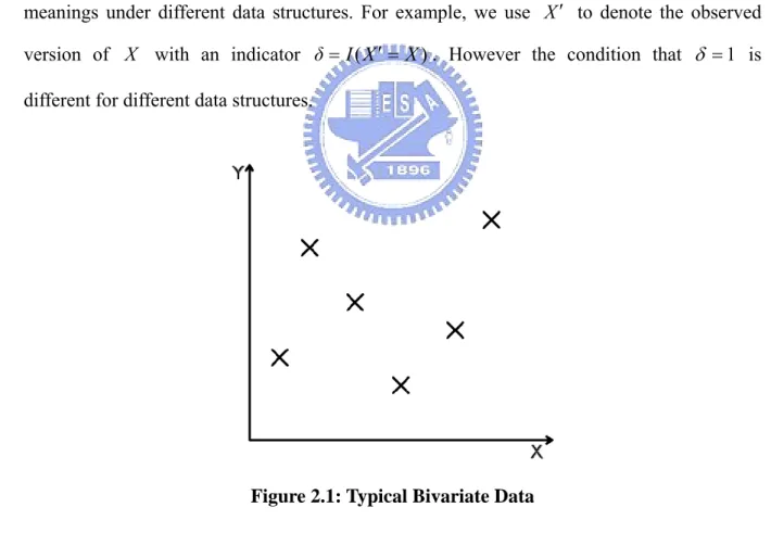
Figure 2.1: Typical Bivariate Data

A. Typical Bivariate Data

Suppose that (X,Y) represent lifetimes of twins or failure times occurred to paired organs. For the former, the dependence can be attributed to shared genetic or environmental

factors. For the latter, the relationship may be explained by the same internal biological system of the subject. Figure 2.1 depicts such data in which replications of (X,Y) have no specific restriction.

External censoring may occur to each member of the pair. Let (C₁,C₂) be external

censoring times so that one only observes (X ′,Y ,'δ₁,δ₂) such that X′= X ∧C₁ ,

2 C Y

Y′= ∧ , δ₁ =I(X <C₁) and δ₂ =I(Y <C₂), where ∧ denotes the minimum and )

(⋅

I is the indicator function. It is usually assumed that (C₁,C₂) are independent of (X,Y). The observed data can be expressed as

{

(X_i′,Y_i′,δ_1i,δ_2i),(i=1,....,n)

}

, where X_i′=X_i∧C_1i,

i i i Y C

Y′= ∧ ₂ , δ_1i =I(X_i <C_1i) and δ_2i =I(Y_i <C_2i) , are random replicates of )

, ,' ,

(X ′ Y δ₁ δ₂ . This type of data is most commonly seen in the literature of survival analysis.

B. Bivariate Analysis － Semi-competing Risks Data

Consider that (X,Y) represent the time to morbidity and the time to mortality of a specific disease on the same subject, respectively. Hence X is subject to right censoring by

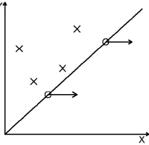
Y but not vice versa. Temporarily we ignore external censoring. Figure 2.2 depicts the structure of semi-competing risks data. Notice that observations of (X,Y) are located on the upper wedge. For those with X > , we only observe Y (X ∧Y=Y,Y) which is located on the diagonal line. This type of data is called “semi-competing risks data” by Fine et al. (2001). When external censoring occurs, it is reasonable to set C₁ =C₂ =C since (X,Y) represent different failure times on the same subject. Usually it is assumed that C is independent of (X,Y). When X is right censored by Y ∧C and Y is right censored by

C, the observed data can be written as {(X_i′,Y_i′,η_i,δ_i),(i=1,....,n)}, where X_i′= X_i∧Y_i ∧C_i,

i i i Y C

Figure 2.2: Semi-competing risks Data

C. Truncation Data

Here we consider a pair of failure times (Y,A) which have a truncation relationship. Specifically we can observe (Y,A) only if Y > . We can say that Y is subject to left A

truncation by A while A is subject to right truncation by Y . Note that, unlike semi-competing risks data, we have no information when Y < . In Figure 2.3, observations A

on the lower wedge will be completely missing and even their existence is unknown. Many applications consider left truncation in which Y is the variable of interest which is subject to truncation by A .

Figure 2.3: Truncation Data

?

2.2 Nonparametric Inferences under Three Data Structures

A. Typical Bivariate Data

For univariate survival data, Kaplan and Meier (1958) expressed the survival function as a product integral of the cumulative hazard function,

) Pr(T >t . ) Pr( )) , [ Pr( 1

∏

≤ ⎭⎬ ⎫ ⎩ ⎨ ⎧ ≥ + ∈ − = t u T u du u u T (2.1)

For the bivariate case, the Kaplan-Meier estimator can be still applied to estimate each of )

Pr(X >x and Pr(Y > y), respectively. When censoring occurs, Pr(X > x) and Pr(Y > y) are estimated based on {(X_i′,δ_1i),(i =1,...,n)} and {(Y_i′,δ_2i),(i =1,...,n)}, respectively. The K-M estimator of Pr(X > and t) Pr(Y > are t)

∏

∑

∑

≤ = = ⎪ ⎪ ⎭ ⎪⎪ ⎬ ⎫ ⎪ ⎪ ⎩ ⎪⎪ ⎨ ⎧ ≥ ′ = = ′ − = > t u n i i n i i i t X I t X I t X 1 1 1 ) ( ) 1 , ( 1 ) r( Pˆ δ ,

∏

∑

∑

≤ = = ⎪ ⎪ ⎭ ⎪⎪ ⎬ ⎫ ⎪ ⎪ ⎩ ⎪⎪ ⎨ ⎧ ≥ ′ = = ′ − = > t u n i i n i i i t Y I t Y I t Y 1 1 2 ) ( ) 1 , ( 1 ) r( Pˆ δ .

Let S(x,y) be the joint survival function of X and Y , where S(x,y) =Pr(X >x,Y > y). There exist several nonparametric estimators of the joint survival function S(x,y). The most well-known one was proposed by Dabrowska (1988).

B. Bivariate Analysis － Semi-competing risks data

With semi-competing risks data, the Kaplan-Meier estimator of Pr(Y > y) is still valid. However, due to dependent censoring, the Kaplan-Meier estimator of Pr(X > x) is biased. Actually the distribution of X is not identifiable nonparametrically.

Suppose that the external censoring is taken into account, one can estimate S(x,y) for

y

, ) ( ˆ ) , ( ) , ( ˆ 1 y G n y Y x X I y x S n i i i

∑

= ≥ ′ ≥ ′ = (2.2) where

∏

∑

∑

≤ = = ⎪ ⎪ ⎭ ⎪⎪ ⎬ ⎫ ⎪ ⎪ ⎩ ⎪⎪ ⎨ ⎧ ≥ ′ = = ′ − = y u n i i n i i i u Y I u Y I y G 1 1 ) ( ) 0 , ( 1 ) ( ˆ δ _.

However, to recover the dependence structure between X and Y , we not only need a valid estimator of S(x,y) but also both of the marginal estimators as well. This implies that the dependence structure can not be recovered non-parametrically for semi-competing risks data. Therefore most authors have considered semi-parametric inference to investigate the dependence structure. The common model assumption is the Archimedean copula family which will be discussed in Section 2.3. We also adopt this approach in the thesis.

C. Truncation Data

Estimating the survival function of Y conditional on Y > by the Kaplan-Meier estimator A

may be biased. Under truncation, we observe {(Y_i,A_i),(i=1,...,n)} only if Y_i > A_i. Hence }

,...,

{Y₁ Y_n is no longer a random sample of Y .

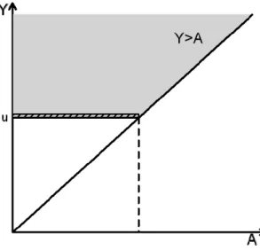
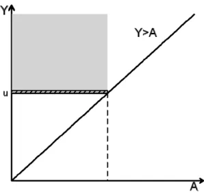
Figure 2.5: Modified Risk Set for Truncation Data

Figure 2.4 explains the truncation mechanism on the hazard estimation. After truncation, the original risk set

{

Y ≥u

}

becomes

{

Y ≥u,Y > A

}

, the shaded area on Figure 2.4. The failure region

{

Y =u

}

changes to

{

Y =u,Y > A

}

, the slash area on the figure.

If we use the set

{

Y ≥u,Y > A

}

to be the new risk set and

{

Y =u,Y > A

}

to be the new instantaneous risk set, it follows that

[

)

) Pr( )) , [ Pr( ) , Pr( ) , , Pr( ) ( ) ( 1 1 u Y du u u Y A Y u Y A Y du u u Y u Y I u Y I p n i i n i i ≥ + ∈ ≠ > ≥ > + ∈ ⎯→ ⎯ ≥ =

∑

∑

= = _.

The resulting estimator of Pr(Y > tends to over-estimate the true survival function. To t) correct this bias, Lynden-Bell modified the set

{

Y ≥u,Y > A

}

by cutting the set further. Lynden-Bell proposed that the new risk set is

{

Y ≥u,A<u

}

, the shaded area on Figure 2.5. The new instantaneous risk set is

{

Y =u,A<u

}

, the slash area on the figure.

Under the assumption that Y and A are independent, one can show that

) Pr( ) Pr( ) Pr( ) Pr( u Y u Y A u,u Y A u,u Y ≥ = = ≥ ≥ ≥ = .

∏

∑

∑

≤ = = ⎪ ⎪ ⎭ ⎪⎪ ⎬ ⎫ ⎪ ⎪ ⎩ ⎪⎪ ⎨ ⎧ > ≥ > = − = > t u n i i i n i i i A u u Y I A u u Y I t Y 1 1 ) , ( ) , ( 1 ) r( Pˆ , (2.3)

is a valid estimator for Pr(Y > . t)

Suppose that there is an external censoring variable C for Y . It is assumed that C is independent of Y . The observed data are

{

Y_i′,A_i,δ_i),(i=1,...,n)

}

conditional on Y_i′> A_i, where Y_i′=Y_i ∧C_i and δ_i =I(Y_i <C_i). It follows that

) , Pr( ) 1 Pr( A u u Y A ,u u,δ Y > ≥ ′ > = = ′ ) Pr( ) ( Pr ) Pr( ) ( Pr u Y u Y A u,u Y A u,u Y ≥ = = > ≥ > = = .

The resulting Lynden-Bell’s estimator becomes

∏

∑

∑

≤ = = ⎪ ⎪ ⎭ ⎪⎪ ⎬ ⎫ ⎪ ⎪ ⎩ ⎪⎪ ⎨ ⎧ > ≥ ′ > = = ′ − = > t u n i i i n i i i i A u,u Y I A ,u u,δ Y I t Y 1 1 ) ( ) 1 ( 1 ) r( Pˆ . (2.4)

Tsai (1991) claimed that most existing procedures for truncation data are still correct under a weaker assumption of quasi-independence, and then proposed a test to verify this condition. The recent paper by Chaieb et al. (2006) consider the assumption that Y and A are correlated and proposed a semi-parametric inference procedure under a “semi-survival” Archimedean copula model. Note that in the thesis, we only assume quasi-independence between the truncation time A and the survival time Y .

2.3 Copula Models and Archimedean Copula Model

Copula models are often used to describe the association between two failure time variables. For the bivariate case, a copula function can be written as C(u,v), which may be parameterized as C_α( vu, ) for u,v∈

[ ]

0,1 . The Archimedean copula (AC) family is a subclass of copula models. A copula is said to be Archimedean copula (AC) if it can be expressed in the following form,

)} ( ) ( { ) , (_{u v} 1 _{u v} C_α =φ_α− φ_α +φ_{α , (2.5)}

where φ_α :

[ ] [ ]

0,1 → ,0 ∞ satisfying φ_α(1)=0, 0φ_α′ t( )< and φ_α′′ t( )>0. Note that the AC family simplifies the bivariate relationship via the univariate function φ_α(⋅). The function

) (⋅ α

φ is the generator of the copula. Important proporties of AC models have been derived in Genest et al. (1986), Oakes (1989) and Genest et al. (1993).

One of the most well-known AC model is the Clayton model with φ_α(_t)=(_t−α −1) α for some α>0, then

α α

α

α(u,v)={u− +v− −1}−1

C . (2.6) In applications, the copula structure is imposed on (X,Y) such that one can write

)} Pr( ), {Pr( ) , (x y C X x Y y S = _α > > (2.7) Accordingly an AC model defined on the joint survival function can be written as

)}} {Pr( )} {Pr( [ ) , (_{x y} 1 _{X x Y y} S = − > + > α α α φ φ φ .

The AC family has nice analytic properties which are useful for further statistical inference. For example, consider the odds ratio function proposed by Oakes (1989):

y x,y S x x,y S y x x,y S x,y S y x ∂ ∂ ⋅ ∂ ∂ ∂ ∂ ∂ ⋅ = / ) ( / ) ( / ) ( ) ( ) , ( 2 * θ (2.8) For an AC model _θ*(_x,_y) _{can be simplified as (S(x,y)),}

α θ where ). ( / ) ( ) ( * _{v v v v} α α φ φ θ =− ′′ ′ (2.9)

Chapter 3 Review of Semi-Parametric Analysis

In this chapter, we review three semi-parametric inference methods for estimating the copula association parameter under different data structures. In Section 3.1 and 3.2, each inference method will be first applied to bivariate data without censoring and then to a more general situation including external censoring. In addition, the application to semi-competing risks data is also considered. In Section 3.3, two-by-two table method by Wang (2003) is directly applied to semi-competing risks data without censoring. Without losing generality, we assume there is no tie in the sample for the observed data.

3.1 The Conditional Likelihood Approach

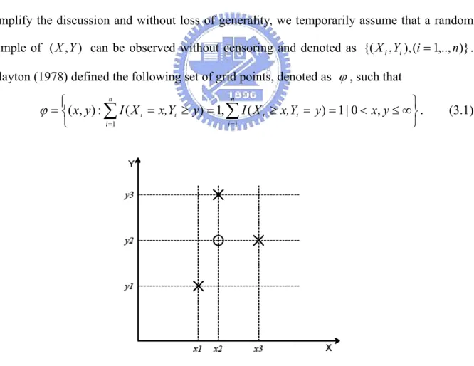
This approach was first proposed by Clayton in his landmark paper (Clayton, 1978). To simplify the discussion and without loss of generality, we temporarily assume that a random sample of (X,Y) can be observed without censoring and denoted as {(X_i,Y_i),(i=1,..,n)}. Clayton (1978) defined the following set of grid points, denoted as ϕ, such that

⎭ ⎬ ⎫ ⎩ ⎨ ⎧ _{= ≥ = ≥ = = < ≤∞} =

∑

∑

= = y x y x,Y X I y x,Y X I y x n i i i n i i i , 0 | 1 ) ( , 1 ) ( : ) , ( 1 1 ϕ . (3.1)

Figure 3.1: An Example of The Set ϕ for An Artificial Data Set

) ,

(x₁ y₁ , )(x₂,y₃ , and (x₃,y₂), marked as “ ╳ ” . According to the definition, the set ϕ consists of four grid points (x₁,y₁), )(x₂,y₃ , )(x₃,y₂ , and (x₂,y₂). Note that (x₂,y₂)

on Figure 3.1 is not an observed failure point. We mark such a point by “

○

”. Define

⎪ ⎪ ⎩ ⎪⎪ ⎨ ⎧ = = > = > = = = = = Δ

∑

∑

∑

= = = . 1 ) , ( and 1 ) , ( if , 0 ; 1 ) , ( if , 1 ) , ( 1 1 1 n i i i n i i i n i i i y Y x X I y Y x X I y Y x X I y x 3.2)

Note that Δ(x,y)=1 implies the grid point (x,y is associated with an observation of ) )

(X, Y (i.e. a point marked by “ ╳ ”). If Δ(x,y)=0, the point (x,y is not an observed point ) (i.e.(x₂,y₂) in the above example and marked by “

○

”). Define

∑

= ≥ ≥ = n i i i y Y x X I y x R 1 ) , ( ) , (

which counts the number at risk at time (x,y . Conditional on the value of ) R(x,y), Δ(x,y) follows a Bernoulli distribution with the probability Pr{Δ(x,y)=1|(x,y)∈ϕ,R(x,y)}. For an AC model, 1 ) , ( )) , ( ( )) , ( ( )} , ( , ) , ( | 1 ) , ( Pr{ − + = ∈ = Δ y x R y x S y x S y x R y x y x α α θ θ ϕ . (3.3)

For the Clayton model with θ_α(S(x,y))=α, we have

1 ) , ( )} , ( , ) , ( | 1 ) , ( Pr{ − + = ∈ = Δ y x R y x R y x y x α α ϕ , (3.4) which does not involve the nuisance parameter S(x,y).

Clayton (1978) suggested that the distribution of Pr{R(x,y)=r|( x,y)∈ϕ} may be ignored in the likelihood construction since it may contain only little information about α . Under a working assumption that Δ(x,y and ) Δ(x ′′,y) are independent for different grid points (x,y and ) ( yx′ ), ′ ∈ϕ , the “conditional” likelihood for an AC model can be written as the product over the conditional probabilities of Δ(x,y for all grid points in the set ) ϕ. Specifically

[

]

[

Pr{ ( , ) 0|( , ) , ( , )}

]

. )} , ( , ) , ( | 1 ) , ( Pr{ )) , ( , ( ) , ( 1 ) , ( ) , ( y x y x y x y x R y x y x y x R y x y x y x S L Δ − ∈ Δ ∈ = Δ × ∈ = Δ =

∏

ϕ ϕ α ϕ _(3.5)

{

}

. 1 ) , ( 1 ) , ( log ) , ( 1 1 ) , ( log ) , ( ) ( ) , (

∑

∈ ⎥⎦ ⎤ ⎢ ⎣ ⎡ ⎟⎟ ⎠ ⎞ ⎜⎜ ⎝ ⎛ + − − Δ − + ⎟⎟ ⎠ ⎞ ⎜⎜ ⎝ ⎛ + − Δ = ϕ α α α α y x R x y y x R y x y x R y x l (3.6)

So that the estimating equation becomes

, 1 ) , ( ) , ( ) ( ) , (

∑

∈ ⎭⎬ ⎫ ⎩ ⎨ ⎧ + − − Δ = ∂ ∂ ϕ α α η η y x R x y y x l _(3.7)

where η =logα . The solution can be denoted as

{

}

∑

∑

∈ ∈ Δ − Δ × − = ϕ ϕ α ) , ( ) , ( ) , ( 1 ) , ( } 1 ) , ( { ˆ y x y x L y x y x y x R .

For general AC models, we can maximize L(α,Sˆ(x,y)), where Sˆ(x,y) is the empirical estimator of S(x,y). However the resulting estimator of α may not have an explicit formula.

When censoring is taken into account, the set ϕ can be modified as

⎭ ⎬ ⎫ = = = ′ ≥ ′ ⎩ ⎨ ⎧

_∑

_{′= ′≥ = =}

_∑

= = 1 ) 1 , , ( , 1 ) 1 , , ( : ) , ( 1 2 1 1 n i i i i n i i i i y Y x X I y Y x X I y x δ δ . (3.8)

The definition of Δ(x,y) is changed to

⎪ ⎪ ⎩ ⎪⎪ ⎨ ⎧ = = = ′ > ′ = = > ′ = ′ = = = = ′ = ′ = Δ

∑

∑

∑

= = = . 1 ) 1 ( , 1 ) 1 ( if , 0 ; 1 ) 1 ( if , 1 ) , ( 1 2 1 1 1 1 2 n i i i i n i i i i n i i i i i y,δ Y x, X I y,δ Y x, X I δ y,δ Y x, X I y x (3.9)

The resulting estimating function under AC model involves the plugged-in estimator, Sˆ(x,y), which can be the Dabrowska’s estimator. The estimator can be modified accordingly. The same principle can also be applied to different data structures, such as semi-competing risks data, in which . ) ( ˆ ) , ( ) , ( ˆ 1 y G n y Y x X I y x S n i i i

∑

= ≥ ′ ≥ ′ =

3.2 Estimating Functions Based on Concordance Indicators

Let )(X_i ,Y_i and (X_j ,Y_j) be independent replications of (X,Y). Define the indicator, 0}

) )(

{( >

=

Δ_ij I X_i-X_j Y_i-Y_j . The two pairs are said to be concordant if Δ =1 and discordant _ij if Δ =0. This indicator reveals dependence relationship between X and Y . Oakes (1989) _ij proposed the following time-dependent association measure：

, ) ~ ~ 0 ( Pr ) ~ ~ 1 ( Pr ) ( y Y x, X | y Y x, X | x,y ij ij ij ij ij ij = = = Δ = = = Δ = θ 0<x,y≤∞ (3.10)

where X~_ij = X_i ∧X_j and Y~_ij =Y_i∧Y_j . For Clayton’s model, we can find that

α

θ(x,y)= for 0< yx, ≤∞ and E(Δ_ij| X~_ij =x,Y~_ij =y)=α/(α+1). The information can be utilized in the inference of α . Assuming the Clayton model, Oakes (1982) proposed the estimating function,

∑ ∑

= > ⎟ ⎠ ⎞ ⎜ ⎝ ⎛ + − = n i j j i ij α α α U 1 ; 1 Δ ) ( . (3.11) The solution can be written as

∑ ∑

∑ ∑

= > = > Δ − Δ = _n i j j i ij n i j j i ij C 1 ; 1 ; ) 1 ( ˆ α

Note that the concordant estimator αˆ is a U-statistic which is useful in the establishment of _C large-sample theory.

To further extend the above idea to incomplete data, the challenge is that some values of

ij

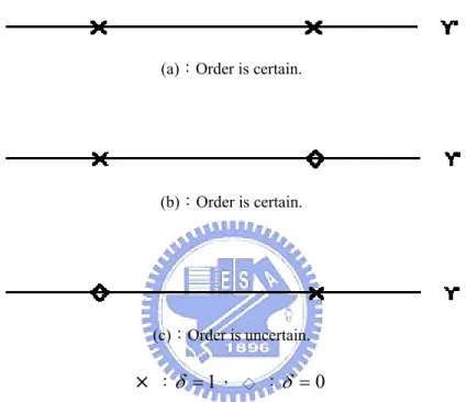
Δ may be uncertain due to censoring. The following discussion is about how the effects of censoring affects the information of Δ . We can write _ij

{( ) 0} {( ) 0}+ {( ) 0} {( ) 0}

ij I X - Xi j I Y -Yi j I X - Xi j I Y -Yi j

This means that to know the value of Δ , we need to know the marginal orders of both _ij )

,

(X_i X_j and (Y_i,Y_j). Given (Y_i′,δ_2i) and (Y_j′,δ_{2 j}), the order of (Y_i,Y_j) is certain if

j i Y

Y′∧ ′ is associated with an uncensored observation. The phenomenon can be explained by the following figures：

(a)：Order is certain.

(b)：Order is certain.

(c)：Order is uncertain.

×

：δ =1， ◇ ：δ =0

Figure 3.2 : The Effect of Censoring on the Order of Two Pairs

Notice that in Figure 3.2 (a) and Figure 3.2 (b), the orders of the two pairs are certain,

while in Figure 3.2 (c) is not. Define that Y~_ij′ =Y_i′∧Y_j′ which is observed if only if it is smaller than both C_2.i and C_2j. Mathematically, we can write the above condition as

ij ij C

Y~ <′ ~₂ , where C~_2ij =C_2i∧C_2j. Similar conclusions can be applied to determine the order of X and _i X . As long as _j X~ <_ij′ C~_1ij, where X~_ij′ = X_i′∧X′_j and C~_ij =C_i∧C_j, the order relationship is certain. Combining the two conditions discussed above, it follows that Δ is _ij certain if both Y~ <_ij′ C~_2ij and X~ <_ij′ C~_1ij are satisfied. Hence for bivariate right censored data,

the condition that the two pairs is “orderable” if Y~_ij′ <C~_2ij and X~_ij′ <C~_1ij. Oakes (1986) defined Z_ij =I(X~_ij <C~_1ij,Y~_ij <C~_2ij) as the indicator of an “orderable” event. This means that Δ can be computable if _ij Z_ij =1. For an AC model,

1 )) ~ , ~ ( ( )) ~ , ~ ( ( ] 1 , ~ , ~ | [ + = = Δ ij ij ij ij ij ij ij ij Y X S Y X S Z Y X E α α θ θ . (3.12)

Under the assumption of Clayton’s model,

1 ] 1 , ~ , ~ | [ + = = Δ α α ij ij ij ij X Y Z E , (3.13) and the resulting estimating function, which has taken censoring into account, can be written as , 1 ) ~ , ~ ( ~ ) ( ~ 1 ;

∑ ∑

= > ⎟ ⎠ ⎞ ⎜ ⎝ ⎛ + − Δ × × = n i j j i ij ij ij ij Z Y X W U α α α _α (3.14)

where )W~ ⋅( is a weight function which is chosen to improve efficiency of the resulting estimator.

For semi-competing risks data with an external censoring, X is right censored by Y or C

and Y is right censored by C. The “orderable” condition becomes X~_ij′ <Y~_ij′ <C~_ij. Fine et al. (2001) defined D_ij =I(X~_ij <Y~_ij <C~_ij) as the indicator of orderable event. For an AC model, we have 1 )) ~ , ~ ( ( )) ~ , ~ ( ( ] 1 , ~ , ~ | [ + = = Δ ij ij ij ij ij ij ij ij Y X S Y X S D Y X E α α θ θ . (3.15)

If Clayton’s model is assumed,

1 ] 1 , ~ , ~ | [ + = = Δ α α ij ij ij ij X Y D E . (3.16) The resulting estimating function becomes:

∑ ∑

= > ⎥⎦ ⎤ ⎢⎣ ⎡ + − Δ × × = n i ij ij i j j ij ij Y D X W U 1 ; 1 ) ~ , ~ ( ) ( α α α _α ,

where W(⋅) is a weight function having the effect on the efficiency as described earlier.

3.3 Estimating Functions Based on Two-by-two Tables

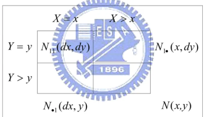
The paper by Day et al. (1997) and Wang (2003) show that the odds ratio of a two-by-two table contains the information of association between (X,Y) at time (x,y). In this section, we directly discuss that the developed estimating function for semi-competing risks data by Wang (2003). To simplify the discussion, we temporarily ignore the external censoring. The observed data are {(X_i′,Y_i,η_i),(i=1,..,n)} , where X′_i = X_i ∧Y_i and

) ( _{i i}

i = I X <Y

η . For a observed point ( yx, ), where y> , we can construct the two-by-two x

table depicted in Figure 3.3.

Figure 3.3 : two-by-two table at time (x,y)

The counts in the cell and the margins can be defined as

, ) , 1 , ( ) , ( 1 11

∑

= = = = ′ = n i i i i y Y x X I dy dx N η ( , ) ( , ), 1 1

∑

= • = ′ ≥ = n i i i y Y x X I dy x N ( , ) ( , 1, ), 1 1

∑

= • = ′= = ≥ n i i i i y Y x X I y dx N η ( , ) ( , .) 1

∑

= ≥ ≥ ′ = n i i i y Y x X I y x N

Given the marginal counts, N₁₁(dx,dy) follows a hyper-geometric distribution with

x X = X >x y Y = N₁₁(dx,dy) N_1•(x,dy) y Y > ) , ( 1 dx y N_• N(x,y)

expectation )} , ( ), , ( ), , ( | ) , ( {N₁₁ dx dy N ₁ dx y N₁ x dy N x y E _{• •} ) , ( ) , ( ) , ( ) , ( ) , ( ) , ( ) , ( 1 1 1 1 y dx N y x N y dx N y x dy x N y dx N y x • • • • − + = α α θ θ (3.17)

Day et al. (1997) and Wang (2003) suggested to construct an estimating functions for α by taking the (weighted) difference between the observed count N₁₁(dx,dy) and its model-based expectation E{N₁₁(dx,dy)|N_•1(dx,y),N_1•(x,dy),

)} , ( yx

N . Under the assumption of no ties and θ_α(x,y)=α, the estimating function can be expressed as

∫∫

⎥ ⎦ ⎤ ⎢ ⎣ ⎡ − + − = ) , ( 11( ) _{( , ) 1} ) , ( ) ( y x N x y dx,dy N y x W U α α α ( ( _{, (3.18)}

Chapter 4 Inference for Semi-competing Risks Data

subject to Left Truncation

In this chapter, we will study a data structure which is a combination of the three data types discussed in Section 2.1. Furthermore, we will propose an inference approach to analyzing this data structure. To simplify the discussion, in Section 4.1 and 4.2 external censoring is ignored. Modification of the proposed method for censored data will be discussed in Section 4.3.

4.1 Data Description

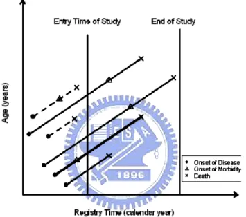
To interpret the data structure studied in this chapter, we use the example of “diabetes diagnosis” which has been introduced in the paper by Peng et al. (2006). After the diagnosis of diabetes, a proportion of patients may suffer from some kind of morbidity, such as nephropathy or retinopathy. The relationship between morbidity and mortality is often of interest. However if researchers only include patients of diabetes who are alive at the time when the study begins, patients who die before the study time will never be included. Such a constraint of the observational scheme tends to exclude patients with shorter survival time after diagnosis. Without taking this fact into account, the subsequent analysis will be biased especially if the proportion of potential patients being excluded in the study is not low.

Using our previous notations, we observe semi-competing risks variables (X ′,Y,η), where Y is the time to mortality and X the time to morbidity , X ′ is maximum of the time to morbidity and mortality, and η =I(X <Y). Let A be the time to the staring date of

the study which is independent of (X,Y). All the three variables are measured from diagnosis of the study. Hence only those with Y > can be included in the sample. Hence A

the observed data are {(X_i′,Y_i,η_i),(i=1,....,n)} only if Y_i > A_i. We assume (X,Y) follow the Clayton model on the upper wedge,

{

Pr( ) Pr( ) 1

}

, ( ) )

,

Pr(_{X > xY > y = X >x} 1−α _{+ Y > y} 1−α ₋ 1/1−α _{x≤ y (4.1)} Figure 4.1 is showed in the paper by Peng et al. (2006). Notice that only those who were alive at the beginning of the study could be included in the sample, i.e. the solid lines on Figure 4.1. Thus two (out of six) persons in the figure will be excluded to the study, i.e. the dashed lines on the figure. The study period in the diagram is long enough to observe the death events of all the subjects in the sample and hence external censoring does not exist.

Figure 4.1: Lexis Diagram for Semi-competing Risks Data subject to Left Truncation

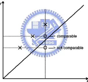
4.2 The Concordance Approach

As we have seen in Section 3.2, an estimating function for the association parameter can be constructed by using the information of the concordance indicator. This approach has been applied to analyze semi-competing risks data subject to left truncation.

Recall that under semi-competing risks data, we know that the information of Δ is _ij based on the orderable condition, X~ <_ij′ Y~_ij, which handles the censoring effect and does not

involve the truncation scheme. For left truncation data, (A,Y is observed only if ) A< . Y

Consider the “comparable event” defined as A(_ij <Y~_ij, where A(_ij =max(A_i,A_j). When this event happens, (A_i ,Y_i) and (A_j ,Y_j) are both located in upper wedge,

} 0

: ) ,

{(a y <a< y<∞ . This means as long as the point (A(_ij,Y~_ij) is located on the upper wedge of the support of (A,Y , where ) Y > , the A (i,j) pairs are comparable. See Figure 4.2 for illustration. Combine the orderable and comparable conditions, which implies that

both X~ <_ij′ Y~_ij and A(_ij <Y~_ij are satisfied, define O_ij =I{(A(_ij ∨X~_ij)<Y~_ij} as the indicator of an “orderable” and “comparable” event.

Figure 4.2: An Example of a Comparable Condition

For an AC model, it follows that

1 )) ~ , ~ ( ( )) ~ , ~ ( ( ] 1 O , ~ , ~ | [ + = = Δ ij ij ij ij ij ij ij ij Y X S Y X S Y X E α α θ θ . (4.2)

For Clayton’s model, we have

1 ] 1 O , ~ , ~ | [ + = = Δ α α ij ij ij ij X Y E , (4.3) Hence the resulting estimating function for the Clayton’s model becomes

∑ ∑

= > ⎥⎦ ⎤ ⎢⎣ ⎡ + − Δ × × = n i ij ij i j j ij ij Y O X W U 1 ; 1 ) ~ , ~ ( ) ( α α α _α , (4.4)

where W(⋅) is a weight function.

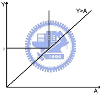
4.3 The Proposed Method Based on Two-by-Two Tables

In this section, we still use the notations of the cell and the margins of the table on Figure 3.3. Recall that in Section 2.2, Lynden-Bell’s estimator uses the idea of further cutting the risk set at Y = by setting y A< . In Figure 4.3, the modified risk set can be written as y

} , : ) , {(a y A≤ y Y ≥ y .

Figure 4.3 : Risk Set for Y modified for Truncation

For an observed failure point with (X,Y)=(x,y), members in the original (unadjusted) risk set include those with {i:X_i ≥x,Y_i ≥ y}. In presence of truncation, we impose additional criteria: {i:A_i ≤ y,Y_i ≥ y}. Subjects fall in the intersection of the two sets will be included in the proposed modified risk set. The corresponding two-by-two table is given below:

Figure 4.3 : The Proposed two-by-two Table at time (x,y)

The definitions of the cells and margins in the table are given as follows:

∑

= < = = = ′ = n i i i i i x η Y y A y X I dy dx N 1 11( , ) ( , 1, , ),

∑

= • = ′≥ = < n i i i i x Y y A y X I dy x N 1 1 ( , ) ( , , ),

∑

= • = ′ = = ≥ < n i i i i i x Y y A y X I y dx N 1 1( , ) ( ,η 1, , ),

∑

= < ≥ ′ ≥ ′ = n i i i i x Y y A y X I y x N 1 ) , , ( ) , ( .

It follows that N₁₁(dx,dy)|N_1•(x,dy) follows a binomial distribution with

) , ( (N_1• x dy ,p₁), where ) 1 Pr( ) 1 Pr( 1 _{′≥ = < =} = < = = ′ = y,η y,A x,Y X y,η y,A x,Y X p . (4.5) Under the assumption that (X,Y) and A are independent, one can show that

) Pr( ) Pr( ) Pr( ) Pr( ) 1 Pr( ) 1 Pr( y x,Y X y x,Y X y y,A x,Y X y y,A x,Y X y,η y,A x,Y X y,η y,A x,Y X = ≥ = = = < = ≥ < = = = = < = ≥ ′ = < = = ′

Similar conclusion for the cell counts, N₀₁(dx,y) follows a binomial distribution with,(N(x,y)−N_1•(x,dy),p₂) where ) Pr( ) Pr( 2 y x,Y X y x,Y X p > ≥ > = = . (4.6) Hence we can find that given the margins counts, N₁₁(dx,dy) still follows a hypergeometric distribution with expectation

)} , ( ), , ( ), , ( | ) , ( {N₁₁ dx dy N ₁ dx y N₁ x dy N x y E _{• •} x X = X >x y A y Y = , < N₁₁(dx,dy) N_1•(x,dy) y A y Y > , < N₀₁(dx,y) ) , ( 1 dx y N_• N(x,y)

) , ( ) , ( ) , ( ) , ( ) , ( ) , ( ) , ( 1 1 1 1 y dx N y x N y dx N y x dy x N y dx N y x • • • • − + = α α θ θ (4.7)

Note that (4.4), (4.5) and (4.6) are derived in appendix. For Clayton’s model with

α y x

θ_α( , )= and under the assumption of no tie and, the estimating function can be expressed as

∫∫

⎥ ⎦ ⎤ ⎢ ⎣ ⎡ − + − = ) , ( 11( ) _{( , ) 1} ) , ( ) ( y x N x y dx,dy N y x W U α α α , (4.8)

where W(x,y) is a weight function.

With semi-competing risks data subject to left truncation and right censoring, the observed data are {(X_i′,Y_i′,η_i,δ_i),(i =1,....,n)}. The definition of the cell and the margins are modified as following：

∑

= < = = ′ = = ′ = n i i i i i i y A y Y x X I dy dx N 1 11( , ) ( ,η 1, ,δ 1, ),

∑

= • = ′ ≥ = = < n i i i i i y A y Y x X I dy x N 1 1 ( , ) ( , ,δ 1, ),

∑

= • = ′ = = ≥ < n i i i i i y A y Y x X I y dx N 1 1( , ) ( ,η 1, , ),

∑

= < ≥ ′ ≥ ′ = n i i i i y A y Y x X I y x N 1 ) , , ( ) , ( .

Chapter 5 Numerical Analysis

In this chapter, we evaluate the finite-sample performance of several estimators via simulation. Here we evaluate semi-competing risks data subject to left truncation. The former analysis ignores external censoring and the latter part includes censoring. As we have assumed that failure time variable (X,Y) follow the Clayton model. Here X and Y is

denoted as the time to morbidity and the time to mortality, respectively. The joint distribution can be expressed as

[

]

[

]

{

Pr( ) Pr( ) 1

}

. ) , Pr(X >x Y > y = X > x 1−α + Y > y 1−α − 1/(1−α)

Let X and Y follow the exponential distribution with parameter λ₁ and λ₂, respectively. We can write ⎪ ⎪ ⎩ ⎪⎪ ⎨ ⎧ − − + − − ⋅ − = − − = − − − − − − _{(1 ) (1 ) ],} ) 1 ( 1 log[ ) 1 ( 1 ], 1 log[ 1 ) 1 ( ) 1 ( ) 1 ( 2 1 α α α α λ α λ V U U Y U X (5.1)

where U ~uniform( 0,1) and V ~uniform( 0,1). In this simulation, we set λ₁ =λ₂ =0.5. The association parameter α is transformed to Kendall’s tau,

1 1 + − = α α τ . (5.2) Given a value of tau, α is produced. The truncation variable A is generated from a exponential distribution with parameter γ . The pair (X,Y) are generated subject to Y > . A

Sample size n are chosen with 100 and 200, respectively. Each combination of α and n

is simulated 1000 times.

(1) Without External Censoring

To fit the constraint of truncation in simulation, we have to decide the percentage of the original population being truncated. According to our simulation settings, we find that

= > )

Pr(Y A γ /(λ₂+γ), (5.3) which means the probability of Y truncated by A is determined by λ and γ . Here if we

let Pr(Y > )A = 50%, we get γ =0.5. We set X ′ = min(X,Y) and the indicator )

(X Y I

η= < . The generated data are {(X_i′,Y_i,A_i,η_i),(i=1,...,n)} conditional on Y_i > A_i. Two types of estimators are evaluated. One is based on the concordance approach:

∑ ∑

= > ⎥⎦ ⎤ ⎢⎣ ⎡ + − Δ × × = n i j j i ij ij ij ij C W X Y O U 1 ; 1 ) ~ , ~ ( ) ( α α α ,

where )O_ij =I((A(_ij ∨ X~_ij)<Y~_ij . Here we consider two weight functions. One is W(x,y)=1 and we denote the corresponding solution as αˆ . The other weight function is _C

n y Y x X I y x W n i i i , )/ ( ) , ( 1

∑

= ≥ ≥ ′ =

and we denote the corresponding solution as α~ . The above estimating function ca be solved _C by the Newton-Raphson algorithm. The second method is our proposal which is based on the two-by-two table approach:

∑

⎥ ⎦ ⎤ ⎢ ⎣ ⎡ − + − = ) ( 11 ( , ) 1 ) ( ) , ( ) ( x,y T W x y N dx,dy _{N x y} U α α α .

We denote the corresponding solution as αˆ_T. The above estimating function is also solved by the Newton-Raphson algorithm.

The results are contained in Table 5.1 ~ Table 5.3. We see that in all the cases, the estimators of the association parameter are unbiased. Numerically the estimated variance is consistent. Especially the proposed estimator αˆ_T has smaller MSE in all the cases with different values of τ which measures the association between X and Y .

Table 5.1: Comparison of the two types of estimators for α with τ =0.75 and in absence of external censoring

Method n=100 n=200 Concordance 0.2481 (1.8595) 0.0833 (0.7483) Weighted Concordance 0.2182 (1.9149) 0.0877 (0.7251) Average Bias (MSE) Two-by-Two Table 0.2248 (1.6624) 0.0879 (0.6569)

Table 5.2: Comparison of the two types of estimators for α with τ =0.5 and in absence of external censoring

Method n=100 n=200 Concordance 0.0407 (0.2667) 0.0220 (0.1347) Weighted Concordance 0.0701 (0.2735) 0.0522 (0.1271) Average Bias (MSE) Two-by-Two Table 0.0564 (0.2458) 0.0400 (0.1189)

Table 5.3: Comparison of the two types of estimators for α with τ =0.25 and in absence of external censoring

Method n=100 n=200 Concordance 0.0209 (0.0756) 0.0165 (0.0352) Weighted Concordance 0.0348 (0.0756) 0.0160 (0.0343) Average Bias (MSE) Two-by-Two Table 0.0296 (0.0685) 0.0343 (0.0316)

(2) With External Censoring

Let C be the censoring variable which follows a exponential distribution with the parameter μ. With censoring taking into account, the truncation criteria becomes conditional on Y′> A, where Y′=min(Y,C). Thus the percentage of the original population being truncated are adjusted as

), /(

)

Pr(Y′ A> =γ λ₂ +μ+γ (5.4) Specially the percentage of the truncated sample being censored by C can be calculated as

) /(

) |

Pr(Y >C Y′> A =μ λ₂ +μ . (5.5) Under the above two conditions the censoring and truncated probabilities can be determined by those three parameters, λ₂,γ,andμ. . Here if we let Pr(Y′> A)= 50% and

= > ′ > | )

Pr(Y C Y A 80%, we get γ =0.625 and μ=0.125. We set X′=min(X,Y,C), the indicator η = I(X <min(Y,C)), Y′=min(Y,C) and the indicator δ =I(Y <C). The generated data are {(X′_i,Y_i′,η_i,δ_i),(i=1,...,n)} conditional on Y_i′> A_i.

Two types of estimators are evaluated. One is based on the concordance approach:

∑ ∑

= > ⎥⎦ ⎤ ⎢⎣ ⎡ + − Δ × × = n i ij ij i j j ij ij C W X Y Q U 1 ; 1 ) ~ , ~ ( ) ( ~ α α α ,

where )Q_ij =I((A(_ij ∨ X~_ij)<Y~_ij <C~_ij . We have considered the two weight functions. One is 1

) , (x y =

W and we denote the corresponding solution as αˆ . The other weight function is _C

n y Y x X I y x W n i i i , )/ ( ) , ( 1

∑

= ≥ ′ ≥ ′ =

and we denote the corresponding solution as α~ . The estimating function is solved by the _C Newton-Raphson algorithm. The second method is based on the two-by-two table approach:

∑

⎥ ⎦ ⎤ ⎢ ⎣ ⎡ − + − = ) ( 11 1 ) , ( ) ( ) , ( ) ( ~ x,y T y x N dx,dy N y x W U α α α .

We denote the corresponding solution as αˆ_T. The above estimating function is also solved by the Newton-Raphson algorithm.

of the association parameter are still unbiased. Numerically the estimated variance is consistent. Especially the proposed estimator αˆ_T has smaller MSE in all the cases with different values of τ which measures the association between X and Y .

Table 5.4: Comparison of the two types of estimators for α with τ =0.75 and in presence of external censoring

Method n=100 n=200 Concordance 0.1477 (2.1712) 0.1521 (1.0069) Weighted Concordance 0.2305 (2.3071) 0.1580 (0.9734) Average Bias (MSE) Two-by-Two Table 0.1770 (2.0012) 0.1449 (0.8757)

Table 5.5: Comparison of the two types of estimators for α with τ =0.5 and in presence of external censoring

Method n=100 n=200 Concordance 0.0894 (0.3635) 0.0337 (0.1546) Weighted Concordance 0.1076 (0.3548) 0.0509 (0.1487) Average Bias (MSE) Two-by-Two Table 0.0965 (0.3250) 0.0424 (0.1361)

Table 5.6: Comparison of the two types of estimators for α with τ =0.25 and in presence of external censoring

Method n=100 n=200 Concordance 0.0274 (0.1025) 0.0080 (0.0431) Weighted Concordance 0.0361 (0.0913) 0.0147 (0.0411) Average Bias (MSE) Two-by-Two Table 0.0338 (0.0865) 0.0121 (0.0379)

Chapter 6 Conclusion

In the thesis, we compare two types of inference procedures for estimating the association parameter of a copula model for semi-competing risks data subject to left truncation. If the truncation mechanism is ignored, the resulting analysis will be biased. We propose a log-rank type estimating function and find that it produces better results in simulations compared with the functions constructed based on the concordance indicators. Both methods involve deletion of some observations in the analysis to eliminate the bias due to truncation. A possible future extension is to utilize all the observations but apply a weighting approach to adjust for the sampling bias.

References

Andersen, P. K. (1988). Multistate Models in Survival Analysis: A study of Nephropathy and Mortality in Diabetes. Statistics in Medicine, 7, 661-670.

Clayton, D. G. (1978). A model for association in bivariate life tables and its application to epidemiological studies of familial tendency in chronic disease epidemiology.

Biometrika, 65, 141-151.

Day, R., Bryant, J. and Lefkopoulon, M. (1997). Adaptation of Biavariate Frailty Models for Prediction, with Application to Biological Markers as Prognostic Indicators. Biometrika,

84, 45-56.

Fine, J. P., Jiang, H., and Chappell, R. (2001). On Semi-competing Risks Data. Biometrika,

88, 907-919.

Genest, C. and Mackay, J. (1986). The Joy of Copulas: Bivariate Distributions with Uniform Marginals. The American Statistician, 40, 280-283.

Jiang, H., Fine, J. P., and Chappell, R. (2005). Semiparametric Analysis of Survival Data with Left Truncation and Dependent Right Censoring. Biometrics, 61, 567-575.

Kaplan, E. L. and Meier, P. (1958). Nonparametric Estimation from Incomplete Observations.

Journal of the American Statistical Association, 53, 457-481.

Klein, J. P. and Moeschberger, M. L. (2003). Survival Analysis : Techniques for Censored

and Truncated data. New York: Springer-Verlag, Second Edition.

Lynden-Bell, D. (1971). A Method of Allowing for Known Observational Selection in Small Samples Applied to 3CR Quasars. Monthly Notices of the Royal Astronomical Society,

155, 95-188.

McCullagh, P. and Nelder, J. A. (1989). Generalized Linear Models. London/Chapman and Hall, Second Edition.

Statistical Society, Series B, 44, 414-422.

Oakes, D. (1986). Semiparametric Inference in a Model for Association in Bivariate Survival Data. Biometrika, 73, 353-361.

Oakes, D. (1989). Bivariate Survival Models induced by Frailties. Journal of the American

Statistical Association, 84, 487-493.

Peng, L. and Fine, J. P. (2006). Nonparametric Estimation with Left-Truncated Semi-competing Risks Data. Biometrika, 93, 367-383.

Wang, W (2003). Estimating the Association Parameter for Copula Models under Dependent Censoring. Journal of the Royal Statistical Society, Series B, 65, 257-273.

Appendix

To simplify the expressions, here we treat (X,Y) as discrete random variables since the probability calculations can be easily converted to the continuous case. It is obvious that

) ), , ( ( ~ ) , ( | ) , ( _{1 1 1} 11 dx dy N x dy BIN N x dy p N _{• •} , where ) Pr( ) 1 Pr( 1 y y,A x,Y X y y,A ,Y x,η X p < = ≥ ′ < = = = ′ = , and ) ), , ( -) , ( ( ~ ) , ( -) , ( | ) ( _{1 1 2} 01 dx,y N x y N x dy BIN N x y N x dy p N _{• •} , where ) Pr( ) 1 Pr( 2 y y,A x,Y X y y,A ,Y x,η X p < ≥ ≥ ′ < ≥ = = ′ = .

Now we show that p₁ and p₂ can be free of the truncation scheme. Under the assumption that (X,Y) and A are independent, one can show that

, ) Pr( ) Pr( ) Pr( ) Pr( ) Pr( ) Pr( ) Pr( ) Pr( ) Pr( ) 1 Pr( ) Pr( ) 1 Pr( 1 y x,Y X y x,Y X y A y x,Y X y A y x,Y X y y,A x,Y X y y,A x,Y X y y,A x,Y Y X y y,A ,Y x,η Y X y y,A x,Y X y y,A ,Y x,η X p = ≥ = = = < = ≥ < = = = < = ≥ < = = = < = ≥ ∧ < = = = ∧ = < = ≥ ′ < = = = ′ = and . ) Pr( ) Pr( ) Pr( ) Pr( ) Pr( ) Pr( ) Pr( ) Pr( ) Pr( ) 1 Pr( ) Pr( ) 1 Pr( 2 y x,Y X y x,Y X y A y x,Y X y A y x,Y X y y,A x,Y X y y,A x,Y X y y,A x,Y Y X y y,A ,Y x,η Y X y y,A x,Y X y y,A ,Y x,η X p > ≥ > = = < > ≥ < > = = < > ≥ < > = = < > ≥ ∧ < > = = ∧ = < > ≥ ′ < > = = ′ =

Since given N(dx,y)=n and N_1•(dx,y)=n_1•, we can know that the variable N₁₁(dx,dy)

is independent of N₀₁(dx,y) intuitively. We have that

) ) , ( , ) , ( , ) , ( | ) , ( Pr(N₁₁ dx dy =n₁₁ N_•1 dx y =n_•1 N dx y =n N_1• dx y =n_1•