動態系統最佳設計數值方法及應用(II)

行政院國家科學委員會專題研究計畫 成果報告

動態系統最佳設計數值方法及應用(2/2)

計畫類別： 個別型計畫

計畫編號： NSC94-2212-E-009-011-

執行期間： 94 年 08 月 01 日至 95 年 07 月 31 日

執行單位： 國立交通大學機械工程學系(所)

計畫主持人： 洪景華

計畫參與人員： 黃智宏，曾錦煥

報告類型： 完整報告

報告附件： 出席國際會議研究心得報告及發表論文

處理方式： 本計畫可公開查詢

中 華 民 國 95 年 8 月 4 日

行政院國家科學委員會補助專題研究計畫

■ 成 果 報 告

□期中進度報告

動態系統最佳設計數值方法及應用

計畫類別：■ 個別型計畫 □ 整合型計畫

計畫編號：NSC93－2212－E009－024

執行期間： 93 年 8 月 1 日至 95 年 7 月 31 日

計畫主持人：洪景華

共同主持人：

計畫參與人員：

成果報告類型(依經費核定清單規定繳交)：□精簡報告 ■完整報告

本成果報告包括以下應繳交之附件：

□赴國外出差或研習心得報告一份

□赴大陸地區出差或研習心得報告一份

□出席國際學術會議心得報告及發表之論文各一份

□國際合作研究計畫國外研究報告書一份

處理方式：除產學合作研究計畫、提升產業技術及人才培育研究計畫、列

管計畫及下列情形者外，得立即公開查詢

□涉及專利或其他智慧財產權，□一年□二年後可公開查詢

執行單位：國立交通大學機械工程研究所

中 華 民 國 九十五 年 八 月 日

摘 要

動態系統所引發的特性一直困擾著工程設計人員，而只在靜態系統模式下，採用最佳

化設計方法所求得的設計，則往往在實際的應用上有所不足。本研究計畫主要依據最佳

設計與最佳控制理論基礎，結合動態分析與數值分析求解技巧，發展一套通用之動態系

統最佳設計方法與軟體。

一般動態系統之最佳化問題可以轉換成標準的最佳控制問題，再透過離散技術轉換成

非線性規劃問題，如此便可利用現有之最佳化軟體進行求解。在本研究計畫中，首先將

動態系統的解題方法與流程發展為最佳控制分析模組，再將該模組與最佳化分析軟體

(MOST) 整合得到整合最佳控制軟體，可以用來解決各種類型的最佳控制問題。為驗證

軟體的效能與準確性，利用本研究計畫所發展之整合最佳控制軟體求解文獻資料中所提

出之各類型最佳控制問題。藉由分析結果之數值與控制軌跡曲線的比對，整合最佳控制

軟體所求出之數值解，在效能與準確性上都能與文獻資料所獲得的最佳解吻合，確認該

整合最佳控制軟體的確可以用來解決我們工程應用上的最佳控制問題。

另外，針對工程設計中存在的離散（整數）最佳控制問題，本研究計畫依據混合整數

非線性規劃法(mixed integer nonlinear programming) 做進一步的研究。猛撞型控制

(bang-bang type control) 是常見的離散最佳控制問題，其複雜與難解的特性更是吸引諸

多文獻探討的主因。許多文獻針對此一問題所提出的方法多在控制函數的切換點數量為

已知的假設條件下所推導，但這並不符合實際工程上的應用需求，因為控制函數的切換

點數量大多在求解完成後才會得知。因此，本研究計畫針對此類型問題發展出兩階段求

解的方法，第一階段先粗略求解該問題在連續空間下的解，並藉此求得控制函數可能的

切換點資訊，第二階段再利用混合整數非線性規劃法求解該問題的真實解。發展過程

中，加強型的分支界定演算法 (enhanced branch-and-bound method)被實際應用並且納入

前一階段所開發的整合最佳控制軟體中，這也使得這個軟體可以同時處理實際動態系統

中最常見的連續及離散最佳控制問題。

最後，本研究計畫將所發展的整合最佳控制軟體用來求解兩個實際的工程應用問題：

飛航高度控制問題與車輛避震系統設計問題。兩個問題都屬於高階非線性控制問題，首

先利用本研究計畫中所建議的解題步驟建構完成這兩個問題的數學模型，接著直接利用

本研究所發展的軟體求解符合問題要求的最佳解。經由這些實際應用案例的驗證，顯示

本研究計畫所發展的方法與軟體的確可以提供工程師、學者與學生一個便利可靠的動態

系統設計工具。

ABSTRACT

The nonlinear behaviors of dynamic system have been of continual concern to both

engineers and system designers. In most applications, the designs – based on a static model

and obtained by traditional optimization methods – can never work perfectly in dynamic cases.

Therefore, researchers have devoted themselves to find an optimal design that is able to meet

dynamic requirements. This project focuses on developing a general-purpose optimization

method, based on optimization and optimal control theory, one that integrates dynamic system

analysis with numerical technology to deal with dynamic system design problems.

A dynamic system optimal design problem can be transformed into an optimal control

problem (OCP). Many scholars have proposed methods to solve optimal control problems and

have outlined discretization techniques to convert the optimal control problem into a

nonlinear programming problem that can then be solved using extant optimization solvers.

This project applies this method to develop a direct optimal control analysis module that is

then integrated into the optimization solver, MOST. The numerical results of the study

indicate that the solver produces quite accurate results and performs even better than those

reported in the earlier literatures. Therefore, the capability and accuracy of the optimal control

problem solver is indisputable, as is its suitability for engineering applications.

A second theme of this project is the development of a novel method for solving

discrete-valued optimal control problems arisen in many practical designs; for example, the

bang-bang type control that is a common problem in time-optimal control problems.

Mixed-integer nonlinear programming methods are applied to deal with those problems in this

project. When the controls are assumed to be of the bang-bang type, the time-optimal control

problem becomes one of determining the switching times. Whereas several methods for

determining the time-optimal control problem (TOCP) switching times have been studied

extensively in the literature, these methods require that the number of switching times be

known before their algorithms can be applied. Thus, they cannot meet practical demands

because the number of switching times is usually unknown before the control problems are

solved. To address this weakness, this project focuses on developing a computational method

to solve discrete-valued optimal control problems that consists of two computational phases:

first, switching times are calculated using existing continuous optimal control methods; and

second, the information obtained in the first phase is used to compute the discrete-valued

control strategy. The proposed algorithm combines the proposed OCP solver with an

enhanced branch-and-bound method and hence can deal with both continuous and discrete

optimal control problems.

Finally, two highly nonlinear engineering problems – the flight level control problem and

the vehicle suspension design problem – are used to demonstrate the capability and accuracy

of the proposed solver. The mathematical models for these two problems can be successfully

established and solved by using the procedure suggested in this project. The results show that

the proposed solver allows engineers to solve their control problems in a systematic and

efficient manner.

目 錄

摘要 ...1

ABSTRACT ... 3

目錄 ...5

LIST OF TABLES ... 6

LIST OF FIGURES ... 7

1. INTRODUCTION ... 8

2. Literature Review and Objectives... 9

Methods for Optimal Control Problems ... 9

Time-Optimal Control Problems ... 11

Objectives ... 12

3. METHODS... 12

3.1 Developing Process of an Multi-Function OCP Solver... 12

3.1.1 Problem formulation... 12

3.1.2 NLP Methods for dynamical optimization ... 13

3.1.3 Computational Algorithm... 14

3.1.4 Systematic Procedure for Solving OCP ... 15

3.2 Mixed-Integer NLP Algorithm for Solving Discrete-valued OCPs ...15

3.3 Algorithm for Solving Discrete-valued OCPs ... 17

3.4 Two-Phase Scheme for Solving TOCP... 18

4. Illustrative Examples... 20

4.1 Third-Order System ... 20

4.2 F-8 Fighter Aircraft... 21

5. Conclusions ... 22

REFERENCES ... 24

計畫成果自評 ...33

附錄 ...36

LIST OF TABLES

LIST OF FIGURES

Figure 1 flow chart of the NLP method for solving OCP... 27

Figure 2 Conceptual layout of the branching process. ... 28

Figure 3 Flow chart of the algorithm for solving discrete-valued optimal control problems. 29

Figure 4 Control trajectories for the third-order system... 30

Figure 5 Control trajectories for the F-8 fighter aircraft. ... 31

Figure 6 Trajectories of the states and control input for the F-8 fighter aircraft. ... 32

1. INTRODUCTION

Two typical methods are usually used to solve optimal control problems: the indirect and

direct approaches. The indirect approach bases on the solution of the first order necessary

conditions for optimality. Pontryagin Minimum Principle (Pontryagin et al. 1962) and the

dynamic programming method (Bellman 1957) are two common methods for indirect

approach. The direct method (Jaddu and Shimemura 1999, Hu et al. 2002, Huang and Tseng

2004) based on nonlinear programming (NLP) approaches that transcribe optimal control

problems into NLP problems and apply existed NLP techniques to solve them. In most of

practical applications, the control problems are described by strongly nonlinear differential

equations that the solutions is hard to be solved by indirect methods. For those cases, the

direct methods can provide another choice to find the solutions.

In spite of extensive use of direct and indirect methods to solve optimal control problems,

engineers still spend much effort on reformulating problems and implementing corresponding

programs for different control problems. For engineers, this routine job will be tedious and

time-consuming. Therefore, a systematic computational procedure for various optimal

control problems has become an imperative for engineers, particularly for those who are

inexperienced in optimal control theory or numerical techniques. Hence, the purpose of this

project is to apply NLP techniques to implement an OCP solver that facilitates engineers in

solving optimal control problems with a systematic and efficient procedure. To illustrate the

practicability and convenience of propose solver, a flight control problem with two different

cases is chosen to illustrate the capability for solving optimal control problem of proposed

solver. The results demonstrate the proposed solver can get the solution correctly and the

procedure suggested in this project can facilitate engineers to deal with their problems.

In many practical engineering applications, the control action is restricted to a set of

discrete values that forms a discrete-valued control problem. These systems can be classified

as switched systems consisting of several subsystems and switching laws that orchestrate the

active subsystem at each time instant. Optimal control problems (OCPs) for switched systems,

which require solution of both the optimal switching sequences and the optimal continuous

inputs, have recently drawn the attention of many researchers. The primary difficulty with

these switched systems is that the range set of the control is discrete and hence not convex.

Moreover, choosing the appropriate elements from the control set in an appropriate order is a

nonlinear combinatorial optimization problem. In the context of time optimal control

problems, as pointed out by Lee et al. (1997), serious numerical difficulties may arise in the

process of identifying the exact switching points. Therefore, an efficient numerical method is

still needed to determine the exact control switching times in many practical engineering

problems.

This study focuses on developing a numerical method to solve discrete-valued optimal

control problems and the time-optimal control problem that is one of their special cases. The

proposed algorithm, which integrates the admissible optimal control problem formulation

(AOCP) with an enhanced branch-and-bound method (Tseng et al., 1995), is implemented and

applied to some example systems.

2. Literature Review and Objectives

Methods for Optimal Control Problems

Optimal control problems can be solved by a variational method (Pontryagin et al., 1962)

or by nonlinear programming approaches (Huang and Tseng, 2003, 2004; Hu et al., 2002;

Jaddu and Shimemura, 1999). The variational or indirect method is based on the solution of

first-order necessary conditions for optimality obtained from Pontryagin’s maximum principle

(Pontryagin et al., 1962). For problems without inequality constraints, the optimality

conditions can be formulated as a set of differential-algebraic equations, often in the form of a

two-point boundary value problem (TPBVP). The TPBVP can be addressed using many

approaches, including single shooting, multiple shooting, invariant embedding, or a

discretization method such as collocation on finite elements. On the other hand, if the problem

requires that active inequality constraints be handled, finding the correct switching structure,

as well as suitable initial guesses for the state and costate variables, is often very difficult.

Much attention has been paid in the literature to the development of numerical methods

for solving optimal control problems (Hu et al., 2002; Pytlak, 1999; Jaddu and Shimemura,

1999; Teo, and Wu, 1984; Polak, 1971), the most popular approach in this field is the

reduction of the original problem to a NLP problem. Nevertheless, in spite of extensive use of

nonlinear programming methods to solve optimal control problems, engineers still spend

much effort reformulating nonlinear programming problems for different control problems.

Moreover, implementing the corresponding programs for the nonlinear programming problem

is tedious and time consuming. Therefore, a general OCP solver coupled with a systematic

computational procedure for various optimal control problems has become an imperative for

engineers, particularly for those who are inexperienced in optimal control theory or numerical

techniques.

Additionally, in many practical engineering applications, the control action is restricted to

a set of discrete values. These systems can be classified as switched systems consisting of

several subsystems and switching laws that orchestrate the active subsystem at each time

instant. Optimal control problems for switched systems, which require solution of both the

optimal switching sequences and the optimal continuous inputs, have recently drawn the

attention of many researchers. The primary difficulty with these switched systems is that the

range set of the control is discrete and hence not convex. Moreover, choosing the appropriate

elements from the control set in an appropriate order is a nonlinear combinatorial optimization

problem. In the context of time optimal control problems, as pointed out by Lee et al. (1997),

serious numerical difficulties may arise in the process of identifying the exact switching

points. Therefore, an efficient numerical method is still needed to determine the exact control

switching times in many practical engineering problems.

Time-Optimal Control Problems

The TOCP is one of most common types of OCP, one in which only time is minimized

and the control is bounded. In a TOCP, a TPBVP is usually derived by applying Pontryagin’s

maximum principle (PMP). In general, time-optimal control solutions are difficult to obtain

(Pinch, 1993) because, unless the system is of low order and is time invariant and linear, there

is little hope of solving the TPBVP analytically (Kirk, 1970). Therefore, in recent research,

many numerical techniques have been developed and adopted to solve time-optimal control

problems.

One of the most common types of control function in time-optimal control problems is the

piecewise-constant function by which a sequence of constant inputs is used to control a given

system with suitable switching times. Additionally, when the control is bounded, a very

commonly encountered type of piecewise-constant control is the bang-bang type, which

switches between the upper and lower bounds of the control input. When the controls are

assumed to be of the bang-bang type, the time-optimal control problem becomes one of

determining the switching times, several methods for which have been studied extensively in

the literature (see, e.g., Kaya and Noakes, 1996; Bertrand and Epenoy, 2002; Simakov et al.,

2002). However, as already mentioned, in contrast to practical reality, these methods require

that the number of switching times be known before their algorithms can be applied. To

overcome the numerical difficulties arising during the process of finding the exact switching

points, Lee et al. (1997) proposed the control parameterization enhancing transform (CPET),

which they also extended to handle the optimal discrete-valued control problems (Lee et al.,

1999) and applied to solve the sensor-scheduling problem (Lee et al., 2001).

In similar manner, this project focuses on developing a numerical method to solve

time-optimal control problems. This method consists of the two-phase scheme: first,

switching times are calculated using existing optimal control methods; and second, the

resulting information is used to compute the discrete-valued control strategy. The proposed

algorithm, which integrates the admissible optimal control problem formulation with an

enhanced branch-and-bound method (Tseng et al., 1995), is then implemented and applied to

some examples.

Objectives

The major purpose of this project is to develop a computational method to solve the

time-optimal control problems and find the corresponding discrete-valued optimal control

laws. The other purpose of this project is to implement a general OCP solver and provide a

systematic procedure for solving OCPs that provides engineers with a systematic and efficient

procedure to solve their optimal control problems.

3. METHODS

3.1 Developing Process of an Multi-Function OCP Solver

The developing processes of a general purpose solver for dynamical optimization can be

described as follows.

3.1.1 Problem formulation

A dynamical optimization problem can be described by a generalized Bolza problem

formulation: Find the design variables b, the control functions u(t) and terminal time tf which

minimize the object function

0 0 0

( , ( ),

)

( , ( ), ( ), )

J

=

ψ

b x

t

t

+

∫

F

b u

t

x

t

t dt

(1)

subject to the system equations

( , ( ), ( ), ),

t

t t

=

x

&

f b u

x

t

≤

t

≤

t

(2)

with initial conditions

0 0

( )

t

=

( )

x

x b

(3)

functional constraints

( , ( ), )

0;

1,...,

( , ( ), ( ), )

0;

1,....,

J

t

t

i

r

F

t

t t dt

i r

r

ψ

=

′

=

=

⎧

+

_⎨

′

≤

= +

⎩

∫

b x

b u

x

(4)

and dynamic point-wise constraints

( , ( ), ( ), )

0;

1,....,

j

t

t t

j

q

φ

b u

x

≤

=

(5)

where b ∈ R

_{is a vector of the design variables, u(t) ∈ R}

is a vector of the control functions,

and x(t)

∈ R

is a vector of the state variables. The functions f, Ψ

, F

, Ψ

, F

and

φ

are

assumed to be at least twice differentiable.

3.1.2 NLP Methods for dynamical optimization

By applying modeling and optimization technologies, a dynamic system optimization

problem can be re-formulated as an optimal control problem (OCP). Hence, many approaches

used to deal with the OCPs can be also applied to solve the dynamical optimization problems.

Most popular approach in this field turned to be reduction of the original problem to a NLP.

Sequential Quadratic Programming (SQP), one of the best NLP methods for solving

large-scale nonlinear optimization, is applied to solve optimal control problems (see, e.g., Gill

et al. 2002, Betts 2000). Before applying the SQP methods, optimal control problems in

which the dynamics are determined by a system of ordinary differential equations (ODEs) are

usually transcribed into nonlinear programming (NLP) problems by discretization strategies.

Due to the consideration of efficiency, the sequential discretization strategy which only the

control variables are discretized is applied. The resulting formulation is then called the

admissible optimal control problem (AOCP) formulation (Huang and Tseng 2003).

3.1.3 Computational Algorithm

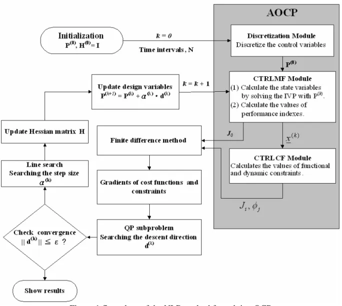
The computational algorithm of the OCP solver which integrates AOCP with SQP is

illustrated in Figure 1 and can be described as the following steps:

Given: Initial values of the design variables vector P

(0)

= [b

, U

, T

] and Number of time

intervals, N.

Initialize iteration counter k :=0 and Hessian Matrix H

:= Identity I.

1. Current design variable vector, P

(k)

, is passed to CTRLMF module of AOCP.

2. Evaluate the values of state variable, x(k), by solving the IVP by substituting P

)

into the

system equation.

(

,

,

, ),

( )

(

)

t

t

=

=

x

f b

u

x

x

x b

&

(6)

3. Compute the values of performance indexes, J

.

0 ( ) ( ) ( ) ( ) ( ) 0 0 ( ) ( ) ( ) 0

(

, (

,

,

, ),

(

,

,

, )

J

t

t

F

t dt

ψ

=

+

∫

b

x b

U

T

b

U

x

(7)

4. Substitute x(k) into Eqs. (4) and (5) to evaluate the values of functional and dynamic

constraints.

5. Evaluate ∇J

, ∇J

, and ∇

φ

by using the finite difference method.

6. Find the descent direction, d

, by solving the QP subproblem.

7. Check convergence criteria, d

≤ ε. If satisfied, stop and show the results.

8. Compute the step size, α

.

9. Update Hessian Matrix H

by applying BFGS method.

10. Update design variables

(k+1)

₌

_{+ ⋅}

_α

P

P

d

(8)

11. Increase iteration counter, k

←

k+1, go back to step 1.

3.1.4 Systematic Procedure for Solving OCP

The following steps describe a systematic procedure for solving the OCP with the proposed

OCP solver:

1. Program formulation: The original optimal control problem must be formulated according

to the extended Bolza formulation.

2. Preparing two parameter files: One of the parameter files describes the numerical schemes

used to solve the OCP and also the relationships between performance index, constraint

functions, dynamic functions, state variables and control variables. The other parameter

file includes the information on SQP parameters, such as convergence parameter,

upper/lower bound and initial guess of design variables, etc.

3. Implementing user-defined subroutines.

4. Execute the optimization: The user defined subroutines are compiled and then linked with

the SQP solver, MOST (Tseng et al., 1996).

5. Execute the optimization.

With the proposed OCP solver, engineers can focus their efforts on formulating their problems

and then follow an efficient and systematic procedure to solve their optimal control problems.

3.2 Mixed-Integer NLP Algorithm for Solving Discrete-valued OCPs

The algorithm developed in this study consists of three major processes: branching, the

AOCP, and bounding. Initially, all discrete-valued restrictions are relaxed and the resulting

continuous NLP problem is solved using the AOCP. If the solution of continuous optimum

design problem occurs when all discrete-valued variable values are in the discrete set U

,

determined and the procedure ends. Otherwise, the algorithm selects one of the

discrete-valued variables whose value is not in the discrete set U

– for example, the j-th

design variable, P

, with value

– and branches on it.

ˆ

P

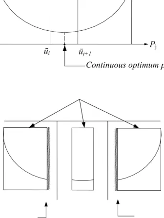
Branching process: In the branching process, the original design domain is divided into

three subdomains by two allowable discrete values, ū

and ū

, that are nearest to the

continuous optimum, as shown in Figure 2. Among the three subdomains, subdomain II,

included in the continuous solution but not in the feasible discontinuous solution, is dropped.

In the other two subdomains, called nodes, two new NLP problems are formed by adding

simple bounds,

P

ˆ

≤

u

_and

P

ˆ

≥

u

_{, respectively, to the continuous NLP problems. One of}

the two new NLP problems is selected and solved next. Many search methods based on tree

searching – including depth-first search, breadth-first search and best-first search – can be

applied to choose the next branching node. The branching process is repeated in each of the

subdomains until the feasible optimal solution is found in which all the discrete variables have

allowable discrete values. Obviously, the number of subdomains may grow exponentially so

that a great deal of computing time is required. Thus in the enhanced branch-and-bound

method (Tseng et al., 1995), multiple branching and unbalanced branching strategies have

been developed to improve the efficiency of the method.

Bounding process: In discrete optimization, the minimum cost is always greater than or

equal to the cost of the original regular optimal design that was originally branched. This fact

provides a guideline for when branching should be stopped. If the branching process yields a

feasible discontinuous solution, then the corresponding cost value can be considered a bound.

Any other subdomain that imposes a continuous minimum cost larger than this bound need

not be branched further. This bounding strategy can be used to select the branching route

intelligently and avoid the need for a complete search over all the branches.

3.3 Algorithm for Solving Discrete-valued OCPs

In this study, the AOCP algorithm is used as the core iterative routine of the enhanced

branch-and-bound method. All candidates will be evaluated and finally an optimal solution

can be found. Here, symbol S is used to represent the discretized control variable set and the P

is the design variable vector. Assuming that the problem at least has one feasible solution, it

can then be proven that an optimal solution exists and can be found by the proposed method.

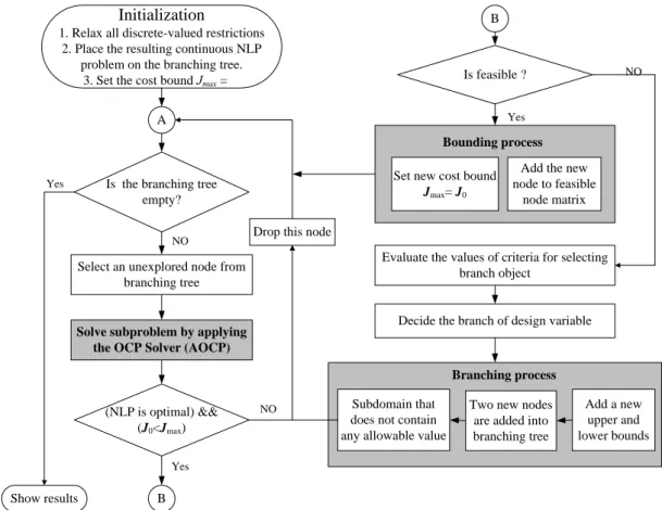
The details of the proposed algorithm are as follows and Figure 3 presents a schematic flow

chart of the algorithm for solving discrete-valued optimal control problems.

Initialization:

Relax all discrete-valued restrictions and then place the resulting continuous NLP problem on

the branching tree.

Set the cost bound J

= ∞.

while (there are pending nodes in the branching tree) do

1. Select an unexplored node from the branching tree.

2. Control discretization.

3. Repeat (for k-th AOCP iteration )

(1). Solve the initial value problem for state variable x

of AOCP.

(2). Calculate the values of the cost function, J

, and the constraints.

(3). Solve the QP

problem by applying the BFGS method to obtain the descent

direction d

.

(4). if (QP

is feasible and convergent) then exit AOCP.

(5). Find the step size α

of the SQP method by using the line search method.

(6). Update the design variable vector: P

(k+1)

_{= P}

P

+ α

(k)

d

.

if (

is feasible ) then

S

Update the current best point by setting the cost bound J

= J

.

Add this node to the feasible node matrix.

else

Evaluate the values of criteria for selecting the branch node.

Choose a discrete-valued variable

S

∉ - and branch it.

Add two new NLP problems into the branching tree.

Drop this node.

endif

else

Stop branching on this node.

endif

end while.

3.4 Two-Phase Scheme for Solving TOCP

The mixed integer NLP algorithm developed in this dissertation is one type of switching

time computation (STC) method. Most switching time computation methods (see, e.g., Kaya

and Noakes, 1996; Lucas and Kaya, 2001; Simakov et al., 2002) assume that the structure of

the control is bang-bang and the number of switching times is known. Unfortunately, the

information on the switchings of several practical time-optimal control problems is unknown

and hard to compute using analytical methods. Hence, to overcome this difficulty, this

dissertation proposes a two-phase Scheme that consists of the AOCP plus the mixed-integer

NLP method. In Phase I, the AOCP is used to calculate the information on switching times

with rough time grids so that the information can be used in Phase II as the feasible initial

design of the mixed integer NLP method. This scheme is described briefly below.

Phase I: Find the information about the switching times and terminal time.

1. Solve the time-optimal control problem using continuous controls by following the

steps of the AOCP method.

2. Based on the numerical results, extract information about the switching times and

terminal time, t

.

Phase II: Calculate the exact solutions

3. Based on the information about switching times obtained in Phase I, treat the

switchings as design variables and add them into the time grid vector T. It should be

noted that each interval between the upper and lower bounds on each of those design

variables must include one switching.

4. Insert the terminal time, t

, into the design variable vector P.

5. Discretize each control variable into the number of switchings plus one. Then the

discrete control vector, S, can be added to the design variable vector P and the

corresponding upper and lower bounds be limited by the original bounds of the

controls.

6. Solve the problem by applying the mixed integer NLP method, and then find the

optimal discrete-type control trajectories.

A third-order system shown in following section is used to demonstrate the processes of this

numerical scheme.

4. Illustrative Examples

The numerical results for the following examples are obtained on an Intel Celeron 1.2

GHz computer with 512 MB of RAM memory. The AOCP is coded in FORTRAN, and C

language is used to implement the enhanced branch-and-bound method. The Visual C++ 5.0

and Visual FORTRAN 5.0 installed in a Windows 2000 operating system are adopted to

compile the corresponding programs. The total CPU times for solving the F-8 fighter craft

problem in Phase I and Phase II are 3.605 and 1.782 seconds, respectively.

4.1 Third-Order System

The following system of differential equations is a model of the third-order system

dynamics taken from Wu (1999).

2 1

x

x

_&

=

,

(9)

x

x

_&

=

,

(10)

10

10

x

_&

= −

x

+

u

.

(11)

The problem here is to find the control |u| ≤ 10 in order to bring the system from the initial

state [-10, 0, 0]

to the final state [0, 0, 0]

in minimum time.

First, this problem is solved directly by the mixed integer NLP method. Assuming four

switching times (T

, T

, T

, T

) and five control arcs have values in the discrete set, U

: {-10,

10}, the terminal time, t

, is treated as a design variable, so the design variable vector P can be

expressed as [T

, T

, T

, T

, t

, U

, U

, U

, U

, U

]

. Most notably, the final conditions of

the state variables are transferred to the equality constraints. Thus, the TOCP problem

becomes one of determining the switching times. Figure 4(a) presents the continuous solution

obtained by using the AOCP and the discrete solution determined by applying the mixed

integer NLP method proposed herein. The results indicate that the control trajectory

determined by the mixed integer NLP method is of the bang-bang type and the solution

consistent with the results obtained by Wu (1999).

As stated in previous section, several assumptions must be made when the mixed integer

NLP method is applied to solving TOCP directly. Unfortunately, these assumptions cannot be

guaranteed to hold in practical cases. Consequently, the two-phase scheme proposed in this

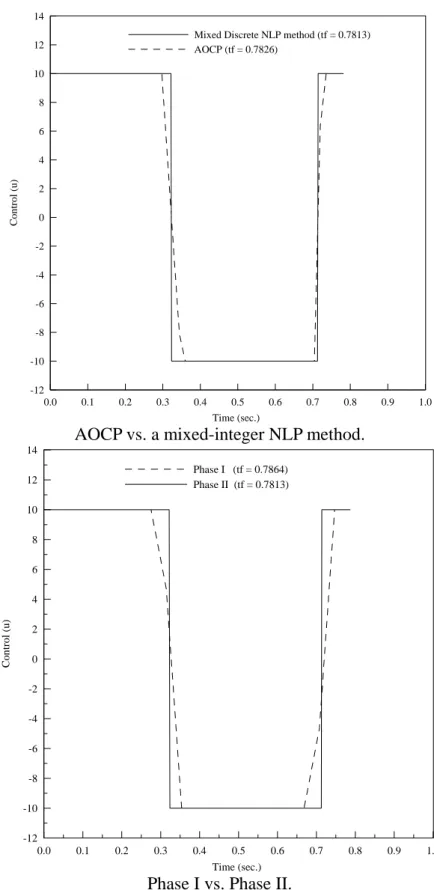
project is needed. For illustration, the third-order system is again solved using this two-phase

scheme. In Phase I, the two switching times are found to be [0.330, 0.725]

and the terminal

time t

is 0.7864. In the first phase, these switching data need not be accurate because they are

only used to help users decide on the number of switching times, the control arcs and their

corresponding boundaries. Thus, in Phase II, the design variable vector P is re-formed as [T

,

T

, t

, U

, U

, U

]

; the numerical result obtained by applying the mixed integer NLP

method is as presented in Figure 4(b). In Phase II, the switching times of the discrete control

input are [0.323, 0.713]

, and the terminal time t

is 0.7813 seconds. The control trajectory

also agrees with that obtained by Wu (1999).

4.2 F-8 Fighter Aircraft

The F-8 fighter aircraft has been considered in several pioneering studies (e.g., Kaya and

Noakes, 1996; Banks and Mhana, 1992; Simakov et al., 2002) and has become a standard for

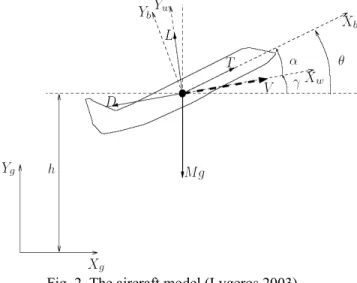
testing various optimal control strategies. A nonlinear dynamic model of the F-8 fighter

aircraft is considered below. The model is represented in state space by the following

differential equations:

0.877

0.088

0.47

0.019

3.846

x

_&

= −

x

+ −

x

x x

+

x

−

x

−

x x

+

x

0.215

u

0.28

x u

0.47

x u

0.63

−

+

−

+

_{u ,}

(15)

x

_&

=

x

,

(16)

4.208

0.396

0.47

3.564

20.967

x

&

= −

x

−

x

−

x

−

x

−

u

(17)

6.265

46

61.4

x u

x u

u

+

+

+

,

where x

is the angle of attack in radians, x

is the pitch angle, x

is the pitch rate and the

control input u represents the tail deflection angle. For convenience of comparison, the

standard settings (Kaya and Noakes, 1996; Lee et al., 1997) are used. A control |u| ≤ 0.05236

must be found that brings the system from its initial state

[

26.7

π

180 ,

0,

0

]

to the final

state

[

0,

0,

0

]

in minimum time.

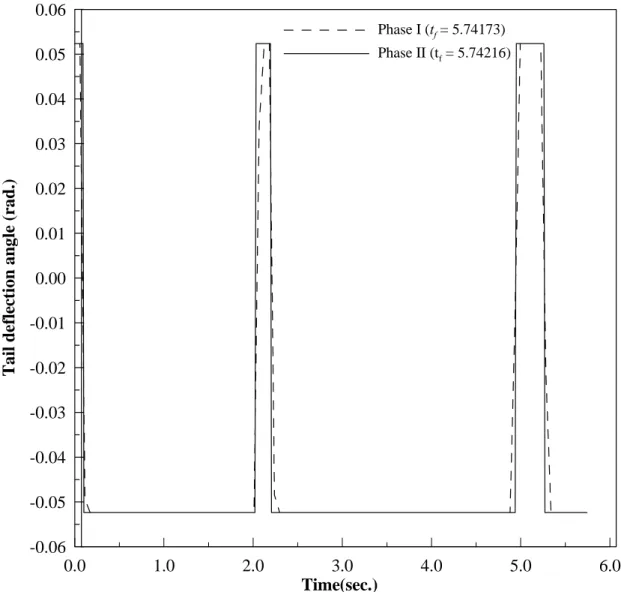
When the two-phase scheme is applied, as described in Section 5.4, the switching times

computed in Phase I are 0.115, 2.067, 2.239, 4.995, and 5.282, and the terminal time is t

=

5.7417. These switching data are used to set the design variables and their corresponding

bounds, and then the problem is solved by the mixed integer NLP method. Finally, the

switching times for the discrete control input are 0.098, 2.027, 2.199, 4.944, and 5.265, and

the terminal time t

is 5.74216. Figure 5 shows the comparison of the controls between Phase I

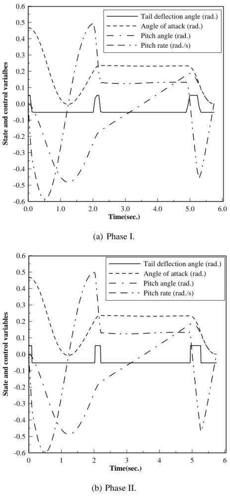
and Phase II, while Figure 6 shows the trajectories of the states and the control of Phase I and

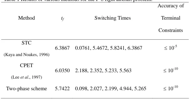
Phase II. This example is also solved by Kaya and Noakes (1996) using the switching time

computation method and by Lee et al. (1997) using the Control Parameterization Enhancing

Transform (CPET) method. Table 1 shows the terminal time t

, switching times and the

accuracy of terminal constraints computed by various methods for this problem. According to

the numerical results, the two-phase scheme provides a better solution, and the accuracy of

the terminal constraints is acceptable.

5. Conclusions

In this project an optimal control problem solver, the OCP solver, based on the

Sequential Quadratic Programming (SQP) method and integrated with many well-developed

numerical routines is implemented. A systematic procedure for solving optimal control

problems is also offered in this project.

This project also presents a novel method for solving discrete-valued optimal control

problems. Most traditional methods focus on the continuous optimal control problems and fail

when applied to a discrete-valued optimal control problem. One common type of such

problems is the bang-bang type control problem arising from time-optimal control problems.

When the controls are assumed to be of the bang-bang type, the time-optimal control problem

becomes one of determining the TOCP switching times. Several methods for such

determination have been studied extensively in the literature; however, these methods require

that the number of switching times be known before their algorithms can be applied. As a

result, they cannot meet practical situations in which the number of switching times is usually

unknown before the control problem is solved. Therefore, to solve discrete-valued optimal

control problems, this dissertation has focused on developing a computational method

consisting of two phases: (a) the calculation of switching times using existing optimal control

methods and (b) the use of the information obtained in the first phase to compute the

discrete-valued control strategy.

The proposed algorithm combines the proposed OCP solver with an enhanced

branch-and-bound method. To demonstrate the proposed computational scheme, the study

applied third-order systems and an F-8 fighter aircraft control problem considered in several

pioneering studies. Comparing the results of this study with the results from the literature

indicates that the proposed method provides a better solution and the accuracy of the terminal

constraints is acceptable.

REFERENCES

Banks, S.P., and Mhana, K.J., “Optimal Control and Stabilization of Nonlinear systems,”

IMA Journal of Mathematical Control and Information, Vol. 9, pp. 179-196, 1992.

Bellman, R., 1957, Dynamic Programming, Princeton University Press, Princeton, NJ, USA.

Betts, J. T., 2000, “Very Low-Thrust Trajectory Optimization Using a Direct SQP Method,”

Journal of Computational and Applied Mathematics, Vol. 120, pp. 27-40.

C.H. Huang, and C.H. Tseng, 2003, “Computational Algorithm for Solving A Class of

Optimal Control Problems,” IASTED International Conference on Modelling,

Identification, and Control (MIC’2003), Innsbruck, Austria, pp. 118-123.

C.H. Huang, and C.H. Tseng, 2004, “Numerical Approaches for Solving Dynamic System

Design Problems: An Application to Flight Level Control Problem,” Proceedings of the

Fourth IASTED International Conference on Modelling, Simulation, and Optimization

(MSO’2004), Kauai, Hawaii, USA, pp. 49-54.

C.H. Tseng, W.C. Liao, and T.C. Yang, 1996, MOST 1.1 User's Manual, Technical Report No.

AODL-93-01, Department of Mechanical Engineering, National Chiao Tung Univ.,

Taiwan, R.O.C.

Gill, P. E., Murray, W., and Saunders, M. A., 2002, “SNOPT: An SQP Algorithm for

Large-Scale Constrained Optimization,” SIAM Journal on Optimization, Vol. 12, No. 4,

pp. 979-1006.

G.S. Hu, C.J. ONG, and C.L. Teo, 2002, “An Enhanced Transcribing Scheme for The

Numerical Solution of A Class of Optimal Control Problems,” Engineering Optimization,

Vol. 34, No. 2, pp. 155-173.

Jaddu, H., and Shimemura, E., 1999, “Computational Method Based on State

Parameterization for Solving Constrained Nonlinear Optimal Control Problems,”

International Journal of Systems Science, Vol. 30, No. 3, pp. 275-282.

Kaya, C.Y., and Noakes, J.L., “Computations and Time-Optimal Controls,” Optimal Control

Applications and Methods, Vol. 17, pp. 171-185, 1996.

Lee, H.W., Jennings, L.S., Teo, K.L., and Rehbock, V., “Control Parameterization Enhancing

Technique for Time Optimal Control Problems,” Dynamic Systems and Applications, Vol.

6, pp. 243-262, 1997.

Lucas, S.K., and Kaya, C.Y., “Switching-Time Computation for Bang-Bang Control Laws,”

Proceedings of the 2001 American Control Conference, pp. 176-181, 2001.

Simakov, S.T., Kaya, C.Y., and Lucas, S.K., “Computations for Time-Optimal Bang-Bang

Control Using A Lagrangian Formulation,” 15th Triennial World Congress, Barcelona,

Spain, 2002.

Pontryagin, L. S., Boltyanskii, V. G., Gamkrelidze, R. V., and Mischenko, E. F., 1962, The

Mathematical Theory of Optimal Processes, Wiley.

Tseng, C.H., Wang, L.W., and Ling, S.F., “Enhancing Branch-And-Bound Method for

Structural Optimization,” Journal of Structural Engineering, Vol. 121, No. 5, pp. 831-837,

1995.

Wu, S.T., “Time-Optimal Control and High-Gain Linear State Feedback,” International

Journal of Control, Vol. 72, No.9, pp. 764-772, 1999.

Table 1 Results of various methods for the F-8 fight aircraft problem.

Method

t

Switching Times

Accuracy of

Terminal

Constraints

STC

(Kaya and Noakes, 1996)

6.3867 0.0761, 5.4672, 5.8241, 6.3867

≤ 10

CPET

(Lee et al., 1997)

6.0350 2.188, 2.352, 5.233, 5.563

≤ 10

ūi

ūi+1

J0

P

Continuous optimum point

Initialization

1. Relax all discrete-valued restrictions 2. Place the resulting continuous NLP

problem on the branching tree. 3. Set the cost bound Jmax=

Is the branching tree empty?

A

Select an unexplored node from branching tree

Solve subproblem by applying the OCP Solver (AOCP)

(NLP is optimal) && (J0<Jmax) B B Yes NO NO Is feasible ?

Drop this node

NO

Yes

Yes

Evaluate the values of criteria for selecting branch object

Decide the branch of design variable

Branching process Two new nodes are added into branching tree Subdomain that

does not contain any allowable value

Add a new upper and lower bounds Bounding process

Add the new node to feasible

node matrix Set new cost bound

Jmax= J0

Show results

0.0 0.1 0.2 0.3 0.4 0.5 0.6 0.7 0.8 0.9 1.0 Time (sec.) -12 -10 -8 -6 -4 -2 0 2 4 6 8 10 12 14 Con tr ol (u)

Mixed Discrete NLP method (tf = 0.7813) AOCP (tf = 0.7826)

AOCP vs. a mixed-integer NLP method.

0.0 0.1 0.2 0.3 0.4 0.5 0.6 0.7 0.8 0.9 1.0 Time (sec.) -12 -10 -8 -6 -4 -2 0 2 4 6 8 10 12 14 Co n tr ol ( u ) Phase I (tf = 0.7864) Phase II (tf = 0.7813)

Phase I vs. Phase II.

0.0

1.0

2.0

3.0

4.0

5.0

6.0

Time(sec.)

-0.06

-0.05

-0.04

-0.03

-0.02

-0.01

0.00

0.01

0.02

0.03

0.04

0.05

0.06

Ta

il

d

e

flec

ti

on

an

g

le

(r

a

d.)

0.0 1.0 2.0 3.0 4.0 5.0 6.0 Time(sec.) -0.6 -0.5 -0.4 -0.3 -0.2 -0.1 0.0 0.1 0.2 0.3 0.4 0.5 0.6 St a te a n d cont r o l v a ria lb e s

Tail deflection angle (rad.) Angle of attack (rad.) Pitch angle (rad.) Pitch rate (rad./s)

(a) Phase I.

Tail deflection angle (rad.) Angle of attack (rad.) Pitch angle (rad.) Pitch rate (rad./s)

(b) Phase II.

計畫成果自評

傳統最佳化設計方法單靠靜態分析所得到產品在實際動態工作環境下往往表現不

佳，甚至有時會面臨無法正常動作的窘境。因此，本研究計畫主要發展目標是依據動態

系統分析與最佳化理論，整合數值分析技巧，發展一套有效率的方法與軟體來協助設計

者處理動態系統最佳設計問題，其中必須將非線性與離散參數設計問題皆需納入考量，

以因應實際工程需求。

本研究計畫分兩年實施，第一年研究重點在於發展出一套整合動態分析與最佳化技

巧的方法，並將之實作成一套泛用型之動態最佳化軟體，此軟體的發展將有助於動態系

統設計者縮短分析及設計的時程，並對產品的更新與市場佔有率的提升提供顯著的幫

助。而要發展一套整合動態分析與最佳化技巧的方法，首先必須解決工程系統非線性的

問題，系統動態特性分析時所解得的系統方程式常常是高度非線性的微分方程組，此時

通常無法求得解析解，而藉助電腦數值分析技巧來求得收斂解是必要的。 第二個困難

點是在於許多動態分析必須藉助專業的分析軟體來進行，此時如何整合最佳化與分析軟

體便成為另一項挑戰。

本計畫利用數值分析方法與程式設計技巧，順利完成預期目標中所要發展的泛用型

之動態最佳化軟體，並利用許多文獻上著名的動態設計與控制問題來進行驗證，從軟體

求得的數值解與文獻的結果作比對，發現本計畫所發展之軟體所得的結果與文獻的結果

是吻合的，甚至有些問題利用本計畫所發展出來的軟體求得的解優於文獻上的結果，由

這些結果我們得到的初步的驗證，也順利完成本計畫中第一年所預期想要達到的目標。

本研究計畫第二年除了延續第一年的主題外，更將工程設計常會遭遇到某些設計尺

寸是有限離散數值（或整數）的情況納入考量。這個看似簡單的問題，其實是讓原本單

純的連續變數最佳化設計問題，轉換成複雜難解的混合型整數最佳化設計問題，但這類

型的問題卻是實際工程上所常常會遭遇的，如果能進一步提供解決這類型的動態最佳化

問題，將可大幅提升研發設計的能力。本研究計畫，採納第一年所發展的解題軟體做為

核心，並將加強型的分支界定演算法 (enhanced branch-and-bound method)納入前一階段

所開發的整合最佳控制軟體中，這也使得這個軟體可以同時處理實際動態系統中最常見

的連續及離散最佳控制問題。

本研究計畫的成果除了實作成功能強大的泛用型動態最佳化分析軟體外，其方法與

應用也發表於國際期刊與會議中。由整個計畫執行過程中，於每個計畫執行階段，計畫

執行所預期之目標均已完成，而整個研究過程中所執行之目標與成果敘述如下：

1. 發展一系統化解決動態最佳化問題的方法與流程，使用者只要依循所建議的方法將

問題定義成標準形式，便可以利用本研究計畫所發展的軟體求得其最佳解。

2. 發展一新穎的方法來求解離散數值最佳控制問題(混合整數之離散數值動態設計問

題)，此方法可以讓使用者在對於原來連續最佳控制問題上對於某些設計變數作些微

的設定修改，就可以求解複雜的離散數值最佳控制問題。

3. 發展一新穎的方法來求解猛撞型的最佳控制問題(Bang-bang Control problems)使用

者無須事先知道控制變數的切換時間點數量，即可求解出最佳的Bang-bang control

law，對於非線性的問題以往要求得其Bang-bang control law是相當困難的，但利用本

研究計畫所發展的方法，搭配數值計算技巧，可以順利求得符合拘束條件的控制法

則。

本研究目前已發表兩篇國際期期刊及兩篇研討會論文

期刊論文

1. C.H. Huang and C.H. Tseng, “An Integrated Two-Phase Scheme for Solving

Bang-Bang Control Problems,” Accepted for publication in Optimization and

Engineering (SCI Expended/ISI).

2. C.H. Huang and C.H. Tseng, “A Convenient Solver for Solving Optimal Control

Problems,” Journal of the Chinese Institute of Engineers, Vol. 28, pp. 727-733, 2005

(Ei/SCI).

研討會論文

1. C.H. Huang, and Tseng, C.H., “Numerical Approaches for Solving Dynamic System

Design Problems: An Application to Flight Level Control Problem,” Proceedings of

the Fourth IASTED International Conference on Modelling, Simulation, and

Optimization (MSO2004), Kauai, Hawaii, USA, 2004, pp. 49-54.

2. C.H. Huang, and Tseng, C.H., “Computational Algorithm for Solving A Class of

Optimal Control Problems,” IASTED International Conference on Modelling,

Identification, and Control (MIC2003), Innsbruck, Austria, 2003, pp. 118-123.

附錄

1. (期刊論文) C.H. Huang and C.H. Tseng, “A Convenient Solver for Solving Optimal

Control Problems,” Journal of the Chinese Institute of Engineers, Vol. 28, pp. 727-733,

2005 (Ei/SCI).

2. (會議論文) C.H. Huang, and Tseng, C.H., “Numerical Approaches for Solving Dynamic

System Design Problems: An Application to Flight Level Control Problem,” Proceedings

of the Fourth IASTED International Conference on Modelling, Simulation, and

Optimization (MSO2004), Kauai, Hawaii, USA, 2004, pp. 49-54.

3. (會議論文) C.H. Huang, and Tseng, C.H., “Computational Algorithm for Solving A Class

of Optimal Control Problems,” IASTED International Conference on Modelling,

Numerical Approaches for Solving Dynamic System Design Problems:

An Application to Flight Level Control Problem

C.H. Huang* and C.H. Tseng**

Department of Mechanical Engineering, National Chiao Tung University Hsinchu 30056, Taiwan, R. O. C. E-mail: chtseng@mail.nctu.edu.tw

TEL: 886-3-5726111 Ext. 55155 FAX: 886-3-5717243 (*Research Assistant, **Professor)

ABSTRACT

The optimal control theory can be applied to solve the optimization problems of dynamic system. Two major approaches which are used commonly to solve optimal control problems (OCP) are discussed in this paper. A numerical method based on discretization and nonlinear programming techniques is proposed and implemented an OCP solver. In addition, a systematic procedure for solving optimal control problems by using the OCP solver is suggested. Two various types of OCP, A flight level tracking problem and minimum time problem, are modeled according the proposed NLP formulation and solved by applying the OCP solver. The results reveal that the proposed method constitutes a viable method for solving optimal control problems.

KEY WORDS

optimal control problem, nonlinear programming, flight level tracking problem, minimum time problem, SQP, AOCP.

1. INTRODUCTION

Over the past decade, applications in dynamic system have increased significantly in the engineering. Most of the engineering applications are modeled dynamically using differential-algebraic equations (DAEs). The DAE formulation consists of differential equations that describe the dynamic behavior of the system, such as mass and energy balances, and algebraic equations that ensure physical and dynamic relations. By applying modeling and optimization technologies, a dynamic system optimization problem can be re-formulated as an optimal control problem (OCP). There are many approaches can be used to deal with these OCPs. In particular, OCPs can be solved by a variational method [1, 2] or by Nonlinear Programming (NLP) approaches [3-5].

The indirect or variational method is based on the solution of the first order necessary conditions for optimality that are obtained from Pontryagin’s Maximum Principle (PMP) [1]. For problems without inequality constraints, the optimality conditions can be formulated as

a set of differential-algebraic equations which is often in the form of two-point boundary value problem (TPBVP). The TPBVP can be addressed with many approaches, including single shooting, multiple shooting, invariant embedding, or some discretization method such as collocation on finite elements. On the other hand, if the problem requires the handling of active inequality constraints, finding the correct switching structure as well as suitable initial guesses for state and co-state variable is often very difficult.

Much attention has been paid to the development of numerical methods for solving optimal control problems [6, 7]. Most popular approach in this field turned to be reduction of the original problem to a NLP. A NLP consists of a multivariable function subject to multiple inequality and equality constraints. The solution of the nonlinear programming problem is to find the Kuhn-Tucker points of equalities by the first-order necessary conditions. This is the conceptual analogy in solving the optimal control problem by the PMP. NLP approaches for OCPs can be classified into two groups: the sequential and the simultaneous strategies. In simultaneous strategy the state and control variable are fully discretized, but in the sequential strategy only discretizes the control variables. The simultaneous strategy often leads the optimization problems to large-scale NLP problems which usually require special strategies to solve them efficiently. On the other hand, instability questions will arise if the discretizations of control and state profiles are applied inappropriately. Comparing to the simultaneous NLP, the sequential NLP is more efficient and robust when the system contains stable modes. Therefore, the admissible optimal control problems which bases on the sequential NLP strategy is propose to solve the dynamic optimization problems in this paper. To facilitate engineers to solve their optimal control problems, a general optimal control problem solver which integrates proposed method with SQP algorithm is developed.

In spite of extensive use of nonlinear programming methods to solve optimal control problems, engineers still spend much effort reformulating nonlinear programming problems for different control problems. Moreover, implementing the corresponding programs of the

nonlinear programming problem is tedious and time-consuming. Therefore, a systematic computational procedure for various optimal control problems has become an imperative for engineers, particularly for those who are inexperienced in optimal control theory or numerical techniques. Hence, the other purpose of this paper is to apply nonlinear mathematical programming techniques to implement a general optimal control problem solver that facilitates engineers in solving optimal control problems with a systematic and efficient procedure.

Flight level tracking plays an important role in autopilot systems receives considerable attentions in many researches [8-12]. For a commercial aircraft, its cruising altitude is typically assigned a flight level by Air Traffic Control (ATC). To ensure aircraft separation, each aircraft has its own flight level and the flight level is separated by a few hundred feet. Changes in the flight level happen occasionally and have to be cleared by ATC. At all other times the aircraft have to ensure that they remain within allow bounds of their assigned level. At the same time, they also have to maintain limits on their speed, flight path angle, acceleration, etc. imposed by limitations of the airframe and engine, passenger comfort requirements, or to avoid dangerous situations such as aerodynamic stall. In this paper, the flight level tracking problem is formulated into an optimal control problem. For safety reasons, the speed of the aircraft and the flight path angle has to be kept in a safe “aerodynamic envelope” [9] and the envelope can be translated into the dynamic constraints of the optimal control problem. A flight level tracking problem and a minimum time problem are shown in Section 5 and then solved by the proposed method.

2. NLP FORMULATION

The formulation of admissible optimal control problems (AOCP) which bases on the sequential strategy is derived by Huang and Tseng [3]. Various types of OCPs are solved successfully by applying AOCP and the formulation is melded with SQP algorithm to develop a general optimal control solver, the OCP solver. Because the NLP formulation based on the AOCP will be applied to solve aircraft flight control problems, a brief description of the NLP formulation and AOCP algorithm is helpful to understand.

Find the design variables P = [bT_{, T}T_{, U}T_]T _{to minimize a}

performance index 0 0

[ , ( , , , ), ]

J

=

y

b x b U T

t

t

_ò

subject to state equations

0

[ , ( , , ), ( , , , ), ] ,

t x

t t dt t

t t

=

£ £

x f b I U T



b U T

0 ( )t = ( ) x h b (3) functional constraints as

[ , ( , , , ), ]

J

=

y

b x b U T

t

t

ò

and dynamic constraints as

0; 1,..., [ , ( , , ), ( , , , ), ] 0; 1,...., j j q t t t j q q f ì_í= = ¢ü_ý ¢ £ = + î þ b I U T x b U T (5)

This NLP formulation presents a general form that includes equality/inequality, functional and dynamic constraints and can be applied to a variety of control problems of engineering applications.

AOCP ALGORITHM

The architectural framework of the OCP solver illustrated in Fig. 1 is composed of SQP and AOCP algorithms. The AOCP algorithm contains three major modules: discretization, CTRLMF and CTRLCF. Each SQP iteration the values of design variable vector P(k) _is

passed into the CTRLMF module to compute the values of state variables by solving the initial value problem and then the values of performance indexes can be evaluated. After the CTRLMF module, the CTRLCF module uses the values of state variables calculated by CTRLMF module to compute the values of constraints. The values of the performance indexes and constraints are also passed back to the SQP algorithm and used to calculate the gradient information. In SQP algorithm, the gradient information will be used to evaluate the convergence and update the design variable vector P(k+1)_{. If the}

convergence criteria are satisfied, the algorithm be stopped and shows the results. SQP is a robust and popular optimization solver and the details can be found in many literatures. Because SQP is the computational foundation of proposed method and hence the convergence and sensitivity of proposed method is same as the convergence and sensitivity of SQP algorithm. The convergence of SQP algorithm has been proposed in many literatures (e.g. [15]). Büskens and Maurer [16] provide a detail description of the sensitivity analysis of SQP method for solving OCP. In this paper, a general optimization solver, MOST [13], which bases on SQP is chosen to develop a general OCP solver.

With admissible optimal control, some good first order differential equation methods having variable step size and error control are available to solve the DAE which is composed of Eqs. (12) and (13), e.g. Adams method and Runge-Kutta-Fehlberg method [14]. These solvers can give accurate results with user desired error control. The state trajectories are internally approximated using interpolation functions in the differential equation solvers. Values of the state and control variables between the grid points can be also obtained with different kinds of interpolation schemes. These numerical schemes are also included and implemented in the proposed OCP solver.