具可延展性以複製為基礎之低複雜度工作排程演算法之研究

國立台中教育大學教育測驗統計研究所理學碩士論文

指導教授：賴冠州 博士

A Study of a Scalable Duplication-based

Task Scheduling Algorithm with Low

Complexity

具可延展性以複製為基礎之低複雜度工

作排程演算法之研究

研 究 生：李佳峯 撰

謝辭

在論文完成的此刻，碩士生涯也隨之圓滿地劃下了句點。回首三年的研究所 生涯，有人覺得唸三年的研究所很浪費時間，但也有許多人對此則是抱持著正面 的想法來看待，有了這些人的鼓勵、支持及協助，讓我在各方面都成長了許多， 心中由衷的感謝曾經幫過我的師長及親友。 本論文承蒙恩師 賴冠州博士悉心指導，不厭其煩的諄諄教誨與深究嚴謹的 指導研究態度，使學生在研究能力、專業觀念、寫作的技巧等都有顯著的提升， 師恩之浩瀚永銘於心，僅致上最大的感恩之意，能遇到這樣的指導教授真的是很 大的一個福報。也感謝口試委員林志敏教授、楊朝棟教授及楊志堅教授，以其專 業的學養與豐富的經驗，在論文的研究上不吝指導，提供了許多非常寶貴的意 見，使本篇論文更加完善與充實，在此也致上由衷的謝意。 感謝學長俊顯，不止在研究上常給予寶貴的意見與協助，還常引導著我一起 激盪出不錯的想法，一起走過的這段光陰，讓我終身難忘。感謝學弟大猷、振偉， 在機器與相關設備上的提供與協助。感謝同學冠志不厭其煩的教導我統計的基本 概念。感謝學妹秀玉的及時雨。感謝學妹才恬總是在我腦筋轉不過來的時候，激 起我其他的研究想法（雖然說她可能不知道），也感謝眾好友的多方幫忙，給予 各方面資源的支援，在此致上最深謝意。最後，謹以本論文獻給我最摯愛的親朋 好友們，謝謝他們在我求學過程中的付出與支持。

Dedication

Table of Contents

List of Figures... iii

List of Tables ...v 摘要 ...vi Abstract... vii Chapter1. Introduction...1 1.1 Motivations...1 1.2 Problems ...2 1.3 Purposes...4 1.4 Restrictions ...7 1.5 Notations...8

Chapter 2. Related Works ...10

2.1 The Levelized Duilication-Based Scheduling (LDBS) Algorithm...10

2.2 The Task Duplication Scheduling (TDS) Algorithm and the Scalable Task Duplication Scheduling (STDS) Algorithm ...11

2.3 The Task Duplication-based Scheduling Algorithm for Network of Heterogeneous Systems (TANH). ...14

2.4 The Heterogeneous Critical Parents with Fast Duplicator (HCPFD) Algorithm ...15

Chapter 3 Proposed Algorithm ...17

3.2 The Dynamic Duplication of Dominate Tasks Scheduling Algorithm...20

Chapter 4. Simulation Environment...32

Chapter 5. Experimental Results...36

5.1 Comparison Metrics ...36

5.2 Influence Factors ...37

5.3 Comparison Results...38

Chapter 6. Conclusions and Future Works...59

List of Figures

Fig. 3-1 An example of unexamined tasks ...21

Fig. 3-2 An example DAG. ...26

Fig. 3-3 Scheduling results for different algorithms ...30

Fig. 4-1 Miniature examples of different task graphs. ...33

Fig. 4-2 Simulation environment...34

Fig. 5-1 Schedule lengths by varying the number of PEs for FFT. ...38

Fig. 5-2 Schedule lengths by varying the number of PEs for LU. ...38

Fig. 5-3 Schedule lengths by varying the number of PEs for GJE...39

Fig. 5-4 Schedule lengths by varying the number of PEs for FORK...39

Fig. 5-5 Schedule lengths by varying the number of PEs for JOIN...40

Fig. 5-6 Average schedule lengths by varying the number of PEs...40

Fig. 5-7 Schedule lengths by varying CCRs for FFT. ...41

Fig. 5-8 Schedule lengths by varying CCRs for LU. ...41

Fig. 5-9 Schedule lengths by varying CCRs for GJE...42

Fig. 5-10 Schedule lengths by varying CCRs for FORK. ...42

Fig. 5-11 Schedule lengths by varying CCRs for JOIN. ...43

Fig. 5-12 Average schedule lengths by varying CCRs. ...44

Fig. 5-13 Schedule lengths by varying the number of pe_var for FFT. ...45

Fig. 5-14 Schedule lengths by varying the number of pe_var for LU. ...45

Fig. 5-15 Schedule lengths by varying the number of pe_var for GJE. ...46

Fig. 5-17 Schedule lengths by varying the number of pe_var for JOIN. ...47

Fig. 5-18 Average schedule lengths by varying the number of pe_var. ...48

Fig. 5-19 Utilization by varying the number of PEs for FFT...49

Fig. 5-20 Utilization by varying the number of PEs for LU. ...49

Fig. 5-21 Utilization by varying the number of PEs for GJE. ...50

Fig. 5-22 Utilization by varying the number of PEs for FORK...50

Fig. 5-23 Utilization by varying the number of PEs for JOIN...51

Fig. 5-24 Average utilization by varying the number of PEs. ...51

Fig. 5-25 Speedup by varying the number of PEs for FFT. ...52

Fig. 5-26 Speedup by varying the number of PEs for LU. ...53

Fig. 5-27 Speedup by varying the number of PEs for GJE...53

Fig. 5-28 Speedup by varying the number of PEs for FORK. ...54

Fig. 5-29 Speedup by varying the number of PEs for JOIN. ...54

List of Tables

Table 1-1 Terms and their meanings...8

Table 3-1 Tasks’ computation costs in different PEs...27

Table 3-2 D3T scheduling step ...29

Table 5-1 Comparison in terms of the schedule length for FFT...55

Table 5-2 Comparison in terms of the schedule length for LU. ...56

Table 5-3 Comparison in terms of the schedule length for GJE. ...56

Table 5-4 Comparison in terms of the schedule length for FORK...56

Table 5-5 Comparison in terms of the schedule length for JOIN...57

摘要

近年來，因科技之發達，有許多需要大量運算之應用已逐步被實現，例如氣 象預報、流體力學、影像處理、甚至於在統計分析上的應用，皆需利用電腦運算 獲得結果。而這些運算中，有些運算模式如 LU、GJE、FFT 是比較常見的運算模 式，這些運算模式可透過平行處理來增進運算速度。 而在平行處理的研究中，分散式異質性系統技術日新月異地進步，但如要使 其能滿足各種平行應用的計算需求，則最需要的就是設計一個有效率的工作排程 策略。過去的研究指出排程問題是一個 NP-complete 的問題；為了考慮排程時間， 許多學者致力於直覺式演算法(Heuristic)的設計。在此論文中則是提出了一個 以複製為基礎的演算法(D3T 演算法)來解決排程問題，其主要精神為考慮每個子 工作排程之後，排程時間最長的路徑會動態的改變。為了使每個階段上會影響總 排程時間的主要子工作(dominate task)所處的排程路徑的排程時間縮短，我們 優先對此主要子工作做排程，以期縮短最後排程時間。透過實驗的證明，D3T 演 算法效能明顯優於其他最近比較有名的演算法(CNPT, TANH, HCPFD)，證明了 D3T 演算法在分散式異質性環境中有不錯的表現，並可達到有效縮短平行程式執行時 間的目標。 關鍵字：靜態工作排程、分散式異質性系統、有向非循環圖、複製基礎

Abstract

Recently, due to the advance of the information technology, many computing sensitive applications have been proposed; for example, weather modeling, statistics analysis, fluid flow, image processing, and so on. Some mathematical expressions are often used in the above applications e.g., the Gauss-Jordan Elimination (GJE), the Fast Fourier Transformation (FFT), LU factoring, and so on. Parallel computing could solve these applications more quickly by creating and coordinating multiple execution processes.

The capability of the distributed heterogeneous computing system grows up in recent years. In order to satisfy the computational requirement of many parallel applications, the most important issue is how to design an efficiently scheduling strategy. However, the scheduling problem is an NP-complete problem; many researchers tend to propose the heuristic to satisfy a reasonable time complexity. This thesis proposes a duplication-based task scheduling algorithm, called D3T, to solve the scheduling problem. The main idea of the D3T algorithm is that the critical path (CP) might dynamically change after each scheduling step. To schedule the dominate task first is a good idea to reduce the schedule length of the critical path.

The experimental results show that the performance of the D3T is better than those of the other three algorithms (CNPT, TANH, HCPFD). The experimental results also demonstrate that the D3T algorithm could reduce the schedule length in the DHC system.

Keyword ： Static task scheduling, distributed heterogeneous computing, directed acyclic graph, duplication-based.

Chapter1. Introduction

1.1 Motivations

Recently, due to the advance of the information technology, many computing sensitive applications have been proposed; for example, weather modeling, statistics analysis, fluid flow, image processing, and so on. These applications generate large-scale data. Analyzing such a huge amount of data takes a lot of time. Some mathematical expressions are often used in the above applications e.g., the Gauss-Jordan Elimination (GJE) (Wu & Gajski, 1990), the Fast Fourier Transformation (FFT) (Chung, Liu, & Liu, 1995), LU factoring (Lord, Kowalik, & Kumar, 1983), and so on. Therefore, researchers need efficient ways to perform these mathematical expressions. Parallel computing could solve these applications more quickly by creating and coordinating multiple execution processes. Before a decade, the most prevalent form of parallel computing is the multiprocessors architecture. As the computational requirement increases rapidly, the computation power of the multiprocessor could not meet the increasing computational requirements. This is because that the multiprocessor architecture has physical limited. Therefore, many institutes use the distributed computing systems instead of the multiprocessor machines. In recent years, the distributed computing systems trends to the distributed heterogeneous computing systems.

machines with different computation capabilities interconnected by high-speed links. Such systems are called the Distributed Heterogeneous Computing (DHC) systems, which executes parallel and distributed applications.

The evolution of network and computing technologies makes the performance of distributed computing systems better in efficacy; thus, the capability of individual machines connected by the high-speed network can even surpass that of the super computer systems. Therefore, the incremental computation capability of the DHC systems becomes an important issue in recent researches.

1.2 Problems

There are parallel applications like weather modeling, fluid flow, image processing. These applications, showing a great deal of adaptable parallelism, make them potential candidates for higher performance computing systems. These computation-intensive applications need more computational capabilities.

In order to fit the computation requirements of parallel applications, the high performance homogeneous computing systems built with dedicated components, often slightly raise the cost-performance ratio. The DHC systems are often composed by the off-the-shelf hardware; therefore, the DHC systems cost less money. Due to the cost of the dedicated DHC computing systems, they are suitable for exploiting heterogeneous resource requirements. When we add new computing components to the DHC system, the new components usually raise the degree of the heterogeneities.

In recent years, the improvement of the network technology also enhances the performance of the DHC systems. Because of the DHC systems that could be constructed by personal computers interconnect by high speed networks, many research institutes change the dedicated computing system to the DHC systems. The DHC systems not only is cheap but also propose more potential and scientific high performance computing systems by congregating a cluster of personal computers in previous literatures. As a result, the DHC systems have been extensively deployed than homogeneous computing systems.

In the DHC system, an application could be partitioned into a set of tasks, and there are relationships among these tasks. In this study, the application is modeled as a Directed Acyclic Graph (DAG), in which each task node represents a sequence of operations and edges represent precedence constraints among these nodes. Task scheduling is to allocate the task nodes to the appropriated computing elements, and to arrange the order of task executions. However, the task scheduling approach could be divided into two categories: the static approach and the dynamic approach. In the static scheduling approach, the characteristics of a parallel program (such as task execution times, data dependencies as the precedence, communication weights) are identified before execution. The scheduling result is produced at compile time（Chu, Lan, & Hellerstein, 1984; Gajski & Peir, 1985）. In the dynamic scheduling approach, only a few information about the parallel application needed before execution, due to that scheduling decisions will be made in running processes （Ahmad & Ghafoor, 1991; Palis et al, 1995）. The scheduling problem is generally an NP-complete

problem.（Garey & Johnson, 1979; Ullman, 1975） Therefore, many heuristics with the acceptable polynomial-time complexity have been proposed (Olivier, Vincent, & Yves, 2002; Sih & Lee,1993; Topcuoglu, Hariri, & Wu, 2002, March; Hagras & Janecek, 2003; Kwok & Ahmad, 2000; Gerasoulis & Yang, 1992; Palis, Liou, & Wei, 1996; Pande, Agrawal, & Mauney, 1994a; Pande, Agrawal, & Mauney, 1995; Ahmad & Kwok, 1998; Bajaj, & Agrawal, 2004; Hagras, & Janecek, 2004a; Hagras, & Janecek, 2004b; Chung, & Ranka, 1992; Liu, 2006; 宋佩珊, 民 92). This thesis focuses on the static approach to solve the compile-time DAG scheduling problem.

1.3 Purposes

The goal of the scheduling algorithm is to allocate the tasks to a system and to arrange the efficient executions to diverse resource requirements. Besides, the scheduling also satisfies the precedence between two tasks. There are various parallelism requirements in the DAG. So that there are thorny challenges to shorten the final completion time and to utilize the heterogeneous resources of the DHC systems in efficient ways.

The static task-scheduling algorithms could be classified into two major groups, heuristic-based and guided random-search-based algorithms (Topcuoglu, Hariri, & Wu, 2002; Liu, Li, Lai, & Wu, 2006). The former claimed heuristic-based algorithms could be further classified into a variety of categories, such as the list-based, clustering-based and duplication-based algorithms.

The list-based scheduling algorithm (Olivier, Vincent, & Yves, 2002; Sih & Lee,1993; Topcuoglu, Hariri, & Wu, 2002, March; Hagras & Janecek, 2003; Kwok & Ahmad, 2000） is generally an attractive approach in terms of low complexity and good performance. Each task is sorted by assigning a priority. The scheduling steps of the list-based approach are to assign priorities statically or dynamically to tasks. In order to minimize the schedule length, the list-based scheduling algorithm repeatedly allocates the tasks to its suitable processing element (PE) with the maximal priority. The main drawback of this approach is that each task is scheduled without sufficient information of subsequent tasks; hence, the priority assignment does not always perform an optimized task scheduling.

The clustering-based approach（Gerasoulis & Yang, 1992; Palis, Liou, & Wei, 1996; Pande, Agrawal, & Mauney, 1994a; Pande, Agrawal, & Mauney, 1995）assumes that there are unbounded number of processors. Then, this method is generally known as a two-phase scheduling.

The basic idea is to reduce the overall communication cost by allocating communicative tasks into one processing element. This approach includes two phases: in the first phase, it groups tasks into an unbounded number of clusters by clustering heuristics, and then allocates these clusters onto the processing elements by load-balancing heuristics. Although the complexity of clustering-based algorithms is generally lower than that of list-based ones, the scheduling performance of clustering-based algorithms is still worse than that of list-based ones.

2004; Hagras, & Janecek, 2004a; Hagras, & Janecek, 2004b; Chung, & Ranka, 1992） is another attractive technique, but the complexity is higher than the previous approaches. The main idea of the duplication-based approach is to duplicate the parents of the candidate nodes to more than one PE. This approach reduces the candidate task’s starting or finishing time by decreasing the communication overhead. The flaws of duplication-based algorithms are the high complexity and redundant resource consumption. In general, duplication-based approaches show their superiority over list-based and clustering ones. However, the improvement from duplicating the parents of a candidate task and the exhausted backward search usually accompanies the cost of increasing complexity.

Guided random search techniques select a choice randomly to get better results in the problem space. The key factor of these techniques is to combine the results of previous searches with some newly randomized parameters to get better results. Genetic algorithms (GAs) (Hou, Ansari, & Ren, 1994; Singh, & Youssef, 1994; Shroff, Watson, Flann, & Freund, 1996; Wang, Siegel, & Roychowdhury, 1996; Correa, Ferreria, & Rebreyend, 1996) are the most extensively used techniques for the task scheduling problem that is different from heuristic algorithms. Although GAs generate good qualities of output schedules, these techniques usually consume much more time than the heuristic-based techniques (Braun, Siegel, Beck, Boloni, Maheswaran, Reuther, Robertson, Theys, Yao, Hengsen, & Freund, 1999). In order to obtain the better quality, the GAs should determine the control parameters appropriately. However, there is no optimal set of control parameters for all

scheduling task graph. Besides GAs, there are other methods like the simulated annealing (Shroff, Watson, Flann, & Freund, 1996; Tao, Narahari, & Zhao, 1993) and the local search method ( Wu, Shu, & Gu, 1997; Kwok, Ahmad, & Gu, 1996 ) in this group.

Due to that the duplication-based scheduling strategies, outperform over the list-based ones in terms of reducing the final schedule length of a DAG, this thesis focuses the duplication-based scheduling strategy on the DHC systems.

1.4 Restrictions

This thesis considers that the classical scheduling algorithms schedule parallel tasks to attain the minimal completion time for a program based on the macro-dataflow model (Sarkar, 1989). The program model assumes an unlimited bandwidth of communications in any point of time. (Bajaj & Agrawal, 2004) (i.e., instantaneous contention-free transmission.). This study will have a further discussion of the restriction in the chapter 3.

The other content of this thesis is organized as follows: first chapter discusses some details about the heuristic algorithm in first section. Chapter 2 presents several duplication-based scheduling algorithms. Chapter 3 introduces our scheduling algorithm. Chapter 4 shows the simulation environment. Chapter 5 demonstrates the experiment results. The conclusions and the future works of this study are

presented in the final chapter.

1.5 Notations

The related terms and the meanings used in this thesis are given in Table 1-1. These symbols will be used in the following chapters.

Table 1-1 Terms and their meanings Term Meaning

DHC Distributed heterogeneous computing DAG Directed acyclic task graph

PE Processor element DT Dominant task CP Critical path SL Schedule length B_level Bottom upward level

CCR The communication to computation ratio ni The ith node (task) of DAG

τi The computation volume of node ni

w(ni) The computation cost of node ni

Ci,j

The communication volume of directed edge form the ni to the

node nj

ei,j

The communication cost of directed edge form the ni to the node

nj

pi The ith processor element

αi The execution rate of processor element p_i

βi The communication rate from processor element pi to processor

element pj

qi,j

The communication channel from processor element pi to

processor element pj

est(ni) The earliest starting time of node ni

ect(ni) The earliest completion time of node ni

EST The earliest starting time AEST(ni,j)

The absolute earliest starting time of node ni on processor element

pj

ALST(ni,j) The absolute latest starting time of node ni on processor element pj

pred(ni) The set of immediate predecessor nodes of node ni

fpred(ni) The favorite predecessor nodes of node ni

Fproc(ni)

The favorite processor of task ni, assigning task ni to the processor

will yield a minimum completion time for task ni

Chapter 2. Related Works

In previous chapter, this thesis has mentioned about three kinds of static scheduling methods (such as the list-based scheduling, the clustering-based scheduling, and the duplication-based scheduling) in heuristic algorithms. Some details of these scheduling approaches would be presented in this chapter. This chapter will introduce five duplication-based algorithms in the DHC systems. The duplication-based algorithms are the Levelized Duilication-Based Scheduling (LDBS) algorithm (Dogan & Ozguner, 2002), the Task Duplication Scheduling (TDS) algorithm (Ranaweera & Agrawal, 2000b), the Scalable Task Duplication Scheduling (STDS) algorithm (Ranaweera & Agrawal 2000a), the Task duplication-based scheduling Algorithm for Network of Heterogeneous systems(TANH) (Bajaj & Agrawal, 2004),and the Heterogeneous Critical Parents with Fast Duplicator (HCPFD) algorithm (Hagras & Janecek, 2004a). These duplication-based algorithms are proposed recently, and some of them can get attractive performance in the DHC systems.

2.1 The Levelized Duilication-Based Scheduling (LDBS)

Algorithm

In this algorithm, the DAG is partitioned into several groups called levels. Tasks in each level are independent of each other. It represents no precedence

between two tasks in the same level. In order to achieve level sorting, the level method uses the depth-first search algorithm for an input DAG. Therefore, all tasks in the same level could be performed in parallel. After the level-sorting phase, this algorithm uses the min_min_heuristic (Braun, et. al., 1999; Wu, Shu, & Zhang, 2000; Wu & Shu, 2001) which is one of the meta-task scheduling algorithms to assign a priority to each task in level 0. In the rest of the LDBS algorithm, each level excluding the level 0 is arranged at each step of the loops. Tasks in the same level are allocated by the duplication_heuristic technique to minimize the schedule length. In the LDBS algorithm, it proposes two versions of the duplication_heuristic phases. The results generated by the two versions of the LDBS algorithm are similar and the time complexities of the two duplication_heuristic approaches are Ｏ( N3 ), where the symbol N represents the number of the tasks in a DAG.

2.2 The Task Duplication Scheduling (TDS) Algorithm

and the Scalable Task Duplication Scheduling (STDS)

Algorithm

The TDS algorithm is the earliest strategy of the TANH algorithm. It contains four steps and they are as follows: the first step traverses the DAG in a top-down fashion to compute the early start time (est), the early completion time (ect), the favorite predecessor (fpred), and the favorite processor (fproc) for each node. In this step, ect(j) is defined to be the smallest value of the ect(j/p), in which the symbol j

represent a task j and the symbol p represents the processor p. The ect(j/p) is the earliest completion time on a processor p. The fproc(j) is the processor such that assigning task j to this processor will get the minimum completion time. The frped is one of the predecessors of the node j and it is the last predecessor to send data to the node j. Besides, the level of each node is obtained by a bottom-up fashion. The level is defined as the highest value of the summation of the computation costs along different paths to the exit node. In the second step, the latest allowable start time (last) and latest allowable completion time (lact) are computed for each node in the bottom-up fashion. The last and lact are used for determining the critical node when performing clustering. The third step arranges all the tasks to the processors by a clustering strategy. Each cluster arranges a path in the DAG. In addition, the number of the clusters is less than that of the available processors under assumption. When arranging a path into a cluster, the path is generated node by node. The first node of the assigned path comes from the first element of the queue and checks its

fpred, that is examined or not. If the fpred is examined, the TDS algorithm would

assign another unexamined predecessor into this cluster. When assigning the predecessor of the selected node, the algorithm would check whether all the predecessor of the node are examined or not. The algorithm will duplicate the fpred into the cluster only if all the predecessors of the current node are assigned. The path is completed by tracing to the entry node. These procedures are repeated until all the nodes are assigned. After the third step, the duplication would be performed for shortening the makespan; and message forwarding is carried out at the same step.

The STDS algorithm is the enhanced version of the TDS algorithm. As mentioned above, The TDS algorithm assumes that the number of the clusters is less than that of the available processors in the clustering phase. However, this assumption is not reasonable because of the required processors may not be enough in practice. The STDS algorithm solves this problem by generating pseudo processors. The computation time of each node on the pseudo processor is set to be the average computation time of the available processors. After each clustering step, the algorithm will check the number of the required processors. If the number of the required processors is more than that of the available ones, it would perform the procedure called the processor_reduction step. The STDS algorithm proposes a merging procedure that merging clusters could gives better performance rather than placing the remaining unassigned tasks on the already created set of clusters. Therefore, the procedure would start to merge two of the produced clusters according to the exec(i) of each cluster. The exec(i) function is defined as the summation of the computation costs of the tasks assigned to the processor i. Otherwise, the algorithm will perform the duplication procedure. The remainder parts of the STDS algorithm are the same as those of the TDS algorithm. The STDS algorithm and the TDS algorithm have the same time complexity, O(v2), where the symbol v indicates the

number of the tasks in the DAG. Although the STDS algorithm could work with a limited set of processors, it still needs a large number of the available processors to perform well in practice.

2.3 The Task Duplication-based Scheduling Algorithm

for Network of Heterogeneous Systems (TANH).

The TANH algorithm is designed based on the cluster-based and the duplication-based approaches. The TANH algorithm extends the STDS algorithm and optimizes the STDS one for several real-life applications. This section quotes the definition of the ect, est, and fp from the STDS algorithm. The TANH algorithm collects some information with some steps in preparation for clustering. The first step is to calculate the est , the ect, and the favorite processors for each node. In the second step, the last, lact, and frped are computed for each node in the bottom-up fashion. The last is defined as the latest allowable start time and the lact is defined as the latest allowable completion time. The fpred represents the favorite predecessor, and the definition of the fpred is different from that of the STDS algorithm. The

fpred is the predecessor that has the minimum completion time compared to other

predecessors of a node. Then, the TANH algorithm generates initial clusters by arranging nodes in ascending order of levels in queue. Each cluster first chooses the unexamined node in queue. Then, the next node for assigning to the same processor is selected from the fpred of the node. This fashion is executed recursively until the selected node is the entry node; if the fpred has been allocated, the unexamined predecessor would be chosen. If all the predecessors are examined, the TANH algorithm would duplicate the fpred to the same cluster in order to minimize the length of the path. These procedures will stop until all nodes that are examined. In the

next step, the TANH algorithm would perform the duplication procedure when the available number of processors is larger than the required number of processors; otherwise, the processor reduction procedure would be carried out when the available number of the processors is smaller than the required number of processors. Finally, the message scheduling is achieved in the last step. The TANH algorithm proposes a different strategy for generating the paths in clustering phase could obtained the nearly optimal makespan.

2.4 The Heterogeneous Critical Parents with Fast

Duplicator (HCPFD) Algorithm

The HCPFD algorithm is extended from the previous work called the CNPT algorithm. In the list phase, The HCPFD algorithm computes the average earliest start time (AEST) and the average latest start time (ALST) for each node in the DAG. In other words, the AEST of a node is the longest length from the entry node to this node. The critical node (CN) is the node, which the AEST and the ALST are the same for the node. After generating the CN, the HCPFD algorithm builds a list queue by choosing the CN first. Before putting the CN into the list queue, all the predecessors of the CN would be put into the list queue to guarantee the satisfaction of the precedence constrain. When all the nodes of the DAG are sorted in the list queue, the machine phase is carried out. The first step of the machine phase puts the node, which is denoted by vi, into the appropriated processor to get the minimum early

completion time (ect). After assigning vi to a processor, the second step finds all

predecessors of vi. Then the second step selects one of the predecessors and the

predecessor is denoted by vcp. The vcp represents the last predecessor that sends the

data to vi gotten from the first step. If duplicating the vcp to the same processor in

which vi stays could raise the early starting time (est) of vi, the duplication procedure

would be executed. The machine assign phase will loop these steps for each node until all the nodes are arranged.

The next chapter will introduce the dynamic duplication of dominate tasks scheduling algorithm.

Chapter 3 Proposed Algorithm

3.1 Problem Definition

As a rule, the classical scheduling algorithms schedule parallel tasks to attain the minimal completion time for a program based on the macro-dataflow model (Sarkar, 1989; Liu, Li, Lai, & Wu, 2006). The program model assumes that the bandwidth of communications that can be performed at the same time is not limited (Bajaj & Agrawal, 2004) (i.e., instantaneous contention-free transmission.). In this study, a program is presented as a directed acyclic graph (DAG) (Liu, Li, Lai, & Wu, 2006). The DAG is defined as G = (N, E, T, C), where N is the set of task nodes, T is the set of node computation volumes (i.e., the unit of the computation volume is “byte”), E is the set of communication edges that define a partial order or precedence constraints on N, and C is the set of communication volumes (i.e., the unit of the communication volume is “byte”). The value τi ∈T is the computation volume for ni ∈ N. The

value of cij ∈ C is the communication volume occurring along the edge eij ∈ E,

where ni, nj ∈ N. Because only static heuristics are discussed here, it is assumed that

the number of executed tasks and the number of PEs in the DHC system are static and known beforehand. In the same way, an accurate estimation of the expected execution volume for each task and that of the expected communication volume between tasks are assumed to be known prior to execution. In this model, this study

assumes that a task is an indivisible unit of computation (i.e., non-preemptive), and that a PE executes one task at a time (i.e., no multitasking). Satisfying precedence constraints and removing resource contentions would trigger tasks’ execution. Precedence constraints occur only when the execution of one task is postponed until all the data from its immediate predecessors arrive. Resource’s contention occurs when a task’s execution is deferred until the completion of all the tasks scheduled before it within the same PE. Suppose that a DHC system is represented as M = (P, Q, A, B), where P={pi|pi∈P, i=1,..,|P|} is the set of heterogeneous PEs, A = {α(pi)|α

(pi)∈A, i=1,..,|P|} is the set of the execution rates for heterogeneous PEs, α(pi) is the

execution rate for pi (i.e., the unit of the execution rate is time/volume, e.g., sec/byte),

Q = {q(pi,pj)|q(pi,pj)∈Q, i, j= 1..|P|} is the set of communication channels, q(pi,pj) is

the communication channel from pi to pj, and B = {β(pi,pj)| β(pi,pj) ∈B, i, j=1..|P|}

is the set of the transferring rates for communication channels from pi to pj (i.e., the

unit of the transfer rate is time/volume, e.g., sec/byte). This study assumes that each PE has a coprocessor to deal with communications, which allow computations and communications that are independent of each other to be overlapped.

Formally, let τi ×α(pj) be the computation cost when task ni is allocated to pj,

and cij×β(pk,pl) be the communication cost from task ni to task nj, where ni is

allocated to pk and task nj is allocated to pl. Given a DAG and a system model as

described above, the scheduling problem is to obtain the minimal-length, non-preemptive schedule of the task graph in the DHC system. To simplify the analysis, the thesis neglects the additional overhead of transforming a serial algorithm

into a parallel form, and assume that no additional processing cost is required to execute programs on DHC systems. Formally, let pred(ni) be the set of immediate

predecessor nodes of ni. The data ready time, drt(ni) of task ni, is defined as the latest

arrival time of communication data from its predecessors (i.e., the data ready time of node ni is the earliest time when the node ni receives all its input data after satisfying

the precedence constraints.). However, after receiving all the input data, a task could not make sure to be triggered its execution. After satisfying the precedence constraint and removing the resource contention, the earliest starting time of node ni,

est(ni) is the earliest time when node ni can start execution. By assuming that ni ∈

pred(nj) is a predecessor node of nj, the earliest completion time of node ni, ect(ni) is

defined as follows:

ect(ni) = est(ni) + τi × α(p(ni)), (1)

where p(ni) ∈ P is the PE that executes ni. Assume that succ(ni) is the set of

immediate successor nodes of ni. Initially, ∀ni ∈ N and pred(ni) = ∅, let est(ni) = 0.

The b-level (Gerasoulis & Yang, 1993; Kwok & Ahmad, 1999) of node ni, b-level(ni)

is the length of the longest path from this node to the sink node. Formally, ∀ ni ∈

N,

b_level(ni)=max(cij ×β +τj×α(nj)+b_level(nj)), (2) where nj∈succ(ni), α(nj) is the average computation rate of task nj, β is the average communication rate, and succ(ni) is the set of immediate successor nodes of ni.

3.2 The Dynamic Duplication of Dominate Tasks

Scheduling Algorithm

Before introducing the Dynamic Duplication of Dominate Tasks scheduling (D3T) algorithm, related terminologies are presented. In the scheduling process, a task is called examined after it is scheduled to some PE and unexamined before it is scheduled to some PE (Liu, Li, Lai, & Wu, 2006). The unexamined tasks can be classified into three sets: (a) the ready set of tasks, in which the immediate predecessors of any ready task are all examined (i.e., the precedence constraints are satisfied and the resource contentions are removed), (b) the partially ready set of tasks, in which at least one of the immediate predecessors of any partially ready task is examined and at least one of its immediate predecessors is unexamined, and (c) the unready set of tasks, in which none of the immediate predecessors of any unready task is examined. Fig. 3-1 shows these situations. After task na is scheduled to some PE, it is examined. The

unexamined set includes {nb, nc, nd, ne}, in which the set {nb, nc} is the ready set, the

a

b

_c

d

examined

unexamined

e

Fig. 3-1 An example of unexamined tasks

Here, the D3T algorithm defines the u-level(ni) of an unexamined ready or partial

ready node ni as the longest length from entry nodes to it. For example,

u_level(nb)=ect(na)+cab×β(p(na)), where β(p(na)) is the average communication rate from p(na) to other PEs. However, after nb and nc are examined,

u_level(nd)= max(ect(na)+cab ×β(p(na)) , ect(nb)+cbd ×β(p(nb)) ,

))) ( ( ) (nc ccd p nc ect + ×β .

Formally, ∀n_j ∈ pred(n_i)∩ examined set, and ∀n_k ∈pred(n_i)∩ unexamined set, ))), ( ( ) ( ) ( _ )), ( ( ) ( max( ) (

_level n_i ect n_j c_ij p n_j u level n_{k k} n_k c_ki p n_k

u = + ×β +τ ×α + ×β (3)

Generally, most of the proposed algorithms fail to consider the problem of exploiting schedule holes (Lai, Fang, Sung, & Pean, 2003; Selvakumar & Murthy, 1994). These occur primarily because of tasks that are scheduled after other tasks with higher scheduling priorities; however, they could be scheduled before those tasks

without affecting their earliest starting times. The D3T algorithm employs these schedule holes by inserting the duplicated parent tasks of a candidate task for advancing the earliest starting time of this candidate task. On the one hand, the utilization of the PE could be raised, and on the other hand, the earliest starting time of some task could be advanced to bring the shortening of the final generated schedule length. To reduce the intermediate schedule length monotonically at each scheduling step to achieve a shorter final schedule length (strict reduction), a dominant task must be identified at each scheduling step. The challenge is to find the selection priority that could well reflect the critical nodes in the context of scheduling. To identify the dominant task in the D3T algorithm, all the ready tasks and the partial ready tasks are considered, and the task ndt with the maximal value of b-level(n_dt) + u-level(n_dt) +

)) (

( dt

dt α p n

τ × is identified as the dominant task (DT).

The main idea of the D3T algorithm is to schedule the CN on the approximated processor and the CN might dynamically change in the task scheduling process. There are two similar algorithms proposed for task scheduling by assigning the CN at each step. They are the Dynamic Critical-Path (DCP) scheduling algorithm (Kwok & Ahmad, 1996) and the Dominate Sequence Clustering (DSC) algorithm (Yang & Gerasoulis, 1994). In the DSC algorithm, the main idea is to reduce the length of the critical path (CP) by edge zeroing in each step. The critical node and its critical predecessor would be merged into the same cluster at each step. Furthermore, the DSC algorithm finds that the result will be better by considering the partial ready nodes. When the platform changes into the DHC system, the DSC algorithm on the

DHC system brings many problems. These difficulties include: (1) how to address the assumption to the unbounded number of processors in the DHC systems, (2) how to assign a partially ready task to the suitable processor, (3) how to obtain the critical path approximately.

The DCP scheduling algorithm utilizes the advantage of the clustering strategy to evaluate the absolute earliest start time (AEST) and the absolute latest start time (ALST). Moreover, the time complexity of the evaluation of considering the AEST and ALST is lower than that of the proposed approaches. The DCP scheduling algorithm also arranges the CN that has the same value of the AEST or ALST to a suitable processor. The strategy of scheduling the CN is different from that of the DSC algorithm. The DCP scheduling algorithm offers an experiment that it might generate very inefficient schedules by making the CN gets the minimum start time. Therefore, the DCP scheduling algorithm uses the looking-ahead strategy to insert the CN behind some examined nodes. There are also some difficulties when the platform changes to the DHC system. The problems are described as follows: (1) how to address the assumption to the unbounded number of processors in the DHC systems, (2) the looking-ahead strategy would raise the time complexity very much used in the DHC systems, (3) how to recalculate the AEST and ALST.

As mentioned above, porting these two algorithms to the DHC systems seems to be very hard. Therefore, researchers start to find another way solving scheduling problem when considering the DHC systems. In recent years, several algorithms are proposed on the DHC system. In order to degrade the complexity, the former

duplication-based algorithms are separated into two phases that are the list and machine assigned phase. The CP would change after allocating a node into a processor, but the two-phase fashion could not solve this situation. The primary idea of the D3T algorithm would like to hold the low time complexity and detects the DT (CN) during allocating period. The DT obtained from the priority function is the critical node in each step. However, the DT node may be in the partially ready set in some steps. At this time, the D3T algorithm would use another priority function that is priority= b-level(ndt) － u-level(ndt) － τdt×α(p(ndt)) to identify the candidate for

scheduling. The priority function is derived as follows: (a) when two tasks are ready and the same value of their b-levels minus computation costs are equal, the task that issued earlier should be scheduled first, (b) when two ready tasks have the same values of their b-levels minus u-levels, the one having the smaller computation cost should also be scheduled first, and (c)when two ready tasks have the same values of their u_levels plus computation costs, the task that could be scheduled to the PE with the larger remainder should be scheduled first. Therefore, the D3T algorithm mingles these three situations to obtain the priority function. Due to the system heterogeneity, a PE that allows the earliest start time is not necessarily the PE that allows the earliest finish time for a node. Recognizing this fact, the D3T algorithm schedules the candidate node, ndt, to the PE that permits its earliest completion time. In this study,

the dominant predecessor (DP) is the predecessor of a task which belongs to the partial ready set or the unready set; when the DP finishes executing, the task’s execution would be triggered by satisfying precedence constraints and removing resource

contentions. In another word, the advance of the earliest starting time of a task would be restricted by the task’s dominant predecessor. The D3T algorithm is presented below. First, the D3T algorithm initializes variables and finds the average execution rates and the average communication rates for all heterogeneous PEs. The D3T algorithm initially assumes that each task is assigned to one virtual PE and that the communication overhead between tasks is assumed to be the average communication rate times the communication volume between tasks. Then the D3T algorithm estimates b-levels for all tasks by using the average execution rates for all heterogeneous PEs bottom-up. Let the tasks without predecessors be in the ready set. When the ready set is not empty, the D3T algorithm repeats the following steps:

1. Calculate the priorities of tasks in the unexamined ready set and partial ready set . The priority function, priority(ni), of a task ni is τi×α(p(ni))+ b-level(ni) +

u-level(ni).

2. Let the dominant task, ndt, be the task with the maximal priority in the ready set and

partial ready set.

3. If ndt belongs to the partial ready set. Then recalculate the priorities of tasks in the

unexamined ready set. The definition priority function is redefine, to priority(ni), of a

task ni is b-level(ni) －τi ×α(p(ni))－ u-level(ni). Then, let the dominant task, ndt,

be the task with the maximal priority in the ready set.

4. Find out the PE, p(ndt), where the ect(ndt) could be obtained.

6. If there is an enough free time slot from drt(ndp) to est(ndt) to schedule ndp to p(ndt),

then schedule the duplicated ndp to p(ndt) to advance the est(ndt) by the insertion

policy.

7. Allocate ndt to p(ndt), and make ndt examined.

8. Re-check the ready set, and re-compute the u-levels for all tasks in the unexamined ready set.

9. Repeat steps 1 to 8 until all tasks are examined.

9 8 8 4 7 3 6 6 3 5 4 6 3 2 6 5 3 4 10 7 8 9 1

Fig. 3-2 An example DAG.

In the following, this study introduces an example to show the superiority of the D3T algorithm. In order to simplify the analyzing process, the D3T algorithm assumes that the computation cost (i.e., τ_i ×α(p(n_i)) ) of all tasks in all PEs are

estimated in the Table 3-1 (e.g., the computation costs of task n1 are 5, 3, 4 in PE1,

PE2, and PE3 respectively), and that the communication rates of all communication channels are all one, therefore the numbers listed along edges are communication volume and also could be considered as the communication costs when the parent node and its child node are scheduled in different PEs (for example, when tasks n1and

n2are scheduled in different PEs, the communication cost between tasks n1 and n2 are

6).

Table 3-1 Tasks’ computation costs in different PEs

PEs Task ni

PE1 PE2 PE3

1 5 3 4 2 3 2 7 3 2 4 9 4 7 5 3 5 8 6 7 6 3 5 7 7 4 2 3 8 2 3 4 9 4 5 3 10 7 3 5

Next, the D3T algorithm could calculate the average computation costs, as listed in Table 3-1. When the set of unexamined tasks is not empty, the D3T algorithm selects one candidate task, ndt, to be scheduled to its corresponding PE. Tasks with no

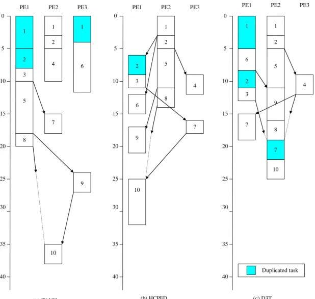
predecessors are selected first. The whole process steps are listed in Table 3-2. The scheduling results obtained from the TANH, HCPDF and D3T algorithms are shown in Fig 3-3.

Table 3-2 D3T scheduling steps

Steps Ready node Priority I Priority II CP node candidate Assigned PE Ect of the candidate Duplication task

1 1 42 1 1 P2 3 2 41 5 41 2 6 37 2 or 5 2 P2 5 5 41 6 37 3 36 3 4 32 5 5 P2 11 6 37 3 36 4 32 4 8 29 6 or 9 6 P1 8 1 3 36 4 32 8 29 5 9 34 3 3 P1 13 2 4 32 8 29 6 9 34 9 9 P2 16 4 32 4 7 8 29 -11 7or 10 4 P3 12 8 29 8 7 33 7or10 7 P1 19 9 8 29 -11 10 8 P2 19 10 10 31 10 10 P2 25 7

(a) TANH

PE1 PE2 PE3

4 1

2

2 5

(b) HCPFD

PE1 PE2 PE3

1 2 5 9 8 2 3 4 (c) D3T PE1 PE2 PE3

3 1 2 4 9 7 8 1 5 6 0 5 10 15 20 25 30 40 35 2 1 0 5 10 15 20 25 30 40 35 0 5 10 15 20 25 30 40 35 1 6 7 7 10 3 7 10 6 8 9 10 Duplicated task

Fig. 3-3 Scheduling results for different algorithms

In the D3T algorithm, the time complexity for calculating the b-level is O((|N|+|E|)|P|). The while loop is executed in O(|N|), finding ndtand its related PE is

O(|N||P|). Finding out the ndp needs O(|N|+|E|) steps. Therefore, the time

Dynamic Duplication of Dominate Tasks scheduling algorithm Input: a DAG G = (N, E, T, C), a DHC system M = (P, Q, A, B) Output: the minimal scheduled length

begin

initialization

let examined(ni)=false, ∀ni ∈ N

let

∑

_jP₌₁α(pj) P , and β(pi,pj)= p pj P pj P P

j i ∀ ∈

∑

=1β( , ) ,

using α(p_i)to compute the b-level bottom-up.

ready_list = ready_list + ni, ∀ni ∈N and pred(ni)=∅ while (ready_list ≠∅) {

let priority(n_i)=b_level(n_i)+τ_i×α(p(n_i))+u_level(n_i),∀ni ∈ready_list

andpartial_ready_list

let ndt = nk, where priority(nk)=max(priority(ni)) If ndt ∈partial_ready_list then

let priority(n_i)=b_level(n_i)−τ_i×α(p(n_i))−u_level(n_i),∀n_i∈ready_list

let ndt = nk, where priority(nk)=max(priority(ni))

End if

find 1. p(ndt), where ect(ndt) could be obtained;

2. ndp for ndt, and their data ready time drt(ndp).

If there is a enough free time slot from drt(ndp) to est(ndt) to schedule ndp to p(ndt),

then schedule the duplicated ndp to p(ndt) to advance the est(ndt) by insertion policy.

Allocate ndt to p(ndt).

ready_list = ready_list - ndt

let examined(ndt)=true

ready_list = ready_list + ni,

) ( _dt

i succ n

n ∈

∀ , if all n_k ∈pred(n_i)∋ _{examined(nk ) = true.}

partial_ready_list=partial_ready_list +nj.

∀n_j ∈succ(n_dt), if ∃nk ∈pred(ni) where examined(nk)= false

Re-compute u-level(ni), where ni ∈ ready_list. }

Chapter 4. Simulation Environment

In this chapter, the simulation environment is described, and five task graphs of the real applications for the simulation environment are introduced. Then the rest of this chapter presents the simulation environment and describes how to generate the system parameters.

To demonstrate the feasibility of the D3T algorithm, the experimental results by evaluating five practical applications are presented in this chapter. The five practical applications includes the Gauss-Jordan Elimination (GJE) (Wu & Gajski, 1990), the Fast Fourier Transformation (FFT) (Chung, Liu, & Liu, 1995), LU factoring (Lord, Kowalik, & Kumar, 1983), Fork trees, and Join trees, whose graph sizes vary from a minimal of 378 nodes to a maximum of 511 nodes. Their miniature examples are shown in Fig. 4-1. The computation/communication volumes required for each task node are pre-determined according to the program structures for different applications.

n1 n2 n5 n3 n9 n6 n7 n4 n8 n10 n11 n1 n2 n3 n5 n9 n6 n7 n4 n8 n10 n11 n2 n5 n3 n9 n6 n7 n4 n8 n12 n13 n14 n15 n1 n10 n11 n1 n2 n5 n3 n9 n6 n7 n4 n8 n12 n14 n13 n15 n10 n11 n1 n2 n3 n5 n9 n6 n7 n4 n8 n12 n13 n14 n15

(a) the LU-decomposition task graph

(b) the Gauss–Jordan Elimination task graph

(c) the Fast Fourier Transformation task graph

(d) the Fork task graph (e) the Join task graph

Fig. 4-1 Miniature examples of different task graphs.

The simulation environment includes three modules: the parameter generator, the task graph generator, and the simulation program with the scheduling algorithms. The simulation environment is illustrated in Fig. 4-2.

Task graph generator Simulation program with Scheduling algorithms Parameter generator Exprimental results

Fig. 4-2 Simulation environment

The parameter generator is for generating the hardware parameters like the computation rates of each node and communication rate of each channel. As mentioned above, a DHC system is represented as M = (P, Q, A, B), where P={pi|pi∈

P, i=1,..,|P|} is the set of heterogeneous PEs, A = {α(pi)|α(pi)∈A, i=1,..,|P|} is the set

of the execution rates for heterogeneous PEs, α(pi) is the execution rate for pi (i.e.,

the unit of the execution rate is time/volume, e.g., sec/byte), Q = {q(pi,pj)|q(pi,pj)∈Q, i,

j= 1..|P|} is the set of communication channels, q(pi,pj) is the communication channel

from pi to pj, and B = {β(pi,pj)| β(pi,pj) ∈B, i, j=1..|P|} is the set of the transferring

rates for communication channels from pi to pj (i.e., the unit of the transfer rate is

time/volume, e.g., sec/byte). This study adopts the consistent heterogeneity approach to model the system heterogeneity (i.e., when any task that runs on a PE faster than another PE implies that the execution time of every task on the previous PE is faster than the execution time on the last PE.). The number of PEs is set to 1, 2, 4, 8, 16, or

32. The variance of the execution rates, α(pi), of the heterogeneous PEs is defined as

the heterogeneity of the computational power. The thesis assumes that the distribution of the execution rate is normally distributed: its mean value is 10, and the variance may be 0.1, 0.3, 0.5, 0.7 or 0.9. The variance of the transfer rates, β(pi,pj),

for communication channels is defined as the heterogeneity of communication mechanisms. This thesis assumes that the distribution of the transfer rate is also normally distributed: its mean value is 10, and the variance may be 0.1, 0.3, 0.5, 0.7 or 0.9. As these variances increase, the system heterogeneities become more obvious. It has long been known that the system heterogeneity may affect the quality of the schedule produced by heuristics.

The task graph generator produces the task graphs for simulating. The simulation program is designed for simulating the scheduling algorithms. The inputs for the simulation program are the task graphs with different parameters in each task graph. The outputs of the simulation program are the schedule lengths obtained after simulating each scheduling algorithm that is executed. Four algorithms e.g., the CNPT algorithm, the HCPFD algorithm, the TANH algorithm, and the D3T algorithm, are included in simulation program.

Chapter 5. Experimental Results

In this chapter, three comparative algorithms, e.g., the CNPT algorithm (Hagras & Janecek, 2003), the TANH algorithm, and the HCPFD algorithm, are applied in the experiment. The CNPT algorithm is a list-based algorithm that schedules tasks according to the task’s priority. In order to demonstrate the differences between the list-based approach and the duplication-based approach, this thesis uses the CNPT and HCPFD algorithms for comparison. As follows, this chapter presents the experimental results to verify the preceding theoretical. Five practical applications are applied to be benchmarks, they are the fork task graph, the join task graph, the FFT task graph, the Gaussian-Jordan elimination task graph, and the LU-decomposition task graph. The comparisons are based on three parameters, e.g., the schedule lengths, the speedup, and the system utilization. In the following, section 5.1 presents the comparison metrics. In section 5.2, the influence factors of the benchmark are described. In section 5.3, the comparison results are illustrated.

5.1 Comparison Metrics

There are three metrics to demonstrate the scheduling performance. The main performance metric is the schedule length (makespan), which is the completion time of the exit node. The next metric is the speedup, which represents the ratio of the sequential execution time to the parallel execution time. The sequential execution

time could be obtained by assigning all tasks to a single PE. The speedup is defined as： makespan p p n speedup P n n i j i j i } )) ( ( min{

∑

_{∈ , ∈} × = α τ

The last metric is the system utilization. In order to consider the usage of the computation resources, the system utilization is defined as：

numbers PE makespan x tasks) duplicated the (include ime executin t tasks' all of sum = n utilizatio

5.2 Influence Factors

Before discussing the experimental results obtained by the simulation system, three dimensions would be focused in the data analysis. The Communication to Computation Ratio (CCR) represents the granularity of the DHC system. There are two types of the granularity. When the communication rate is higher than the computation rate, the granularity of the system is coarse grain. In other words, the value of CCR is bigger than one. In contrast, when the computation rate is higher than the communication rate, the granularity of the system is fine grain. Currently, the value of CCR is smaller than one.

The next influence factor is the number of the PEs. In general, more PEs produce lower makespans. The last influence factor is the processor heterogeneity, which is represented by pe_var. When the value of the distribution of the processor computing cost grows up, it means the execution time of a task that is much different

in each PE.

5.3 Comparison Results

This section discusses the experimental results in each graph to give the research a full view in different situation. The schedule lengths of the four algorithms with different influence factors are shown in the following.

50000 70000 90000 110000 130000 150000 170000 190000 2 4 8 16 32 S ch edul e le ngt h TANH CNPT HCPFD D3T PE #

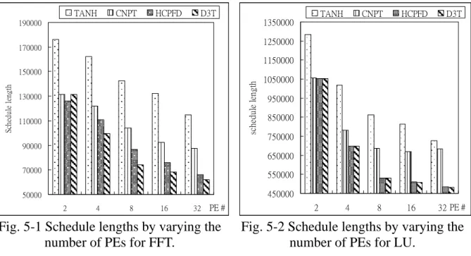
Fig. 5-1 Schedule lengths by varying the number of PEs for FFT.

450000 550000 650000 750000 850000 950000 1050000 1150000 1250000 1350000 2 4 8 16 32 sc hedul e le n gt h TANH CNPT HCPFD D3T PE #

Fig. 5-2 Schedule lengths by varying the number of PEs for LU.

Fig. 5-1~ Fig. 5-6 show that the average schedule lengths generated by the D3T algorithm is monotonically reduced when the number of PEs increases. In Fig. 5-1, the average schedule length obtained by the D3T algorithm is the only case, which generates the longer length than that generated by the HCPFD algorithm when the number of PE is 2. It indicates that the D3T algorithm needs more processors for performing the FFT application. The average schedule lengths obtained by the D3T algorithm are shorter than that obtained by the other three algorithms. In Fig. 5-2, the

average schedule lengths of the CNPT, the HCPFD, and the D3T algorithms are almost the same. This is because that the structure of the LU application has a heavy weight CP. Hence, the tasks in the CP would be allocated into the same processor and the schedule length is hardly changed.

20000 120000 220000 320000 420000 520000 620000 2 4 8 16 32 sc hd ul e le n gt h TANH CNPT HCPFD D3T PE #

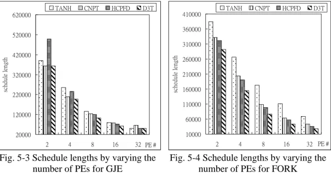
Fig. 5-3 Schedule lengths by varying the number of PEs for GJE

10000 60000 110000 160000 210000 260000 310000 360000 410000 2 4 8 16 32 sc he du le le ng th TANH CNPT HCPFD D3T PE #

Fig. 5-4 Schedule lengths by varying the number of PEs for FORK

In Fig. 5-3, the queer result is observed that the HCPFD algorithm generates the long schedule length when the number of PEs is 2 or 4. After tracing the scheduling position of each task assigned by the HCPFD algorithm, the experimental results show that the worse case with the Gaussian-Jordan elimination task graph is caused by assigning arbitrarily the predecessor of the CN. In Fig. 5-4, the scheduling performance of the D3T algorithm is better than that of the others.

0 50000 100000 150000 200000 250000 300000 350000 2 4 8 16 32 sc hed ul e le n gt h TANH CNPT HCPFD D3T PE #

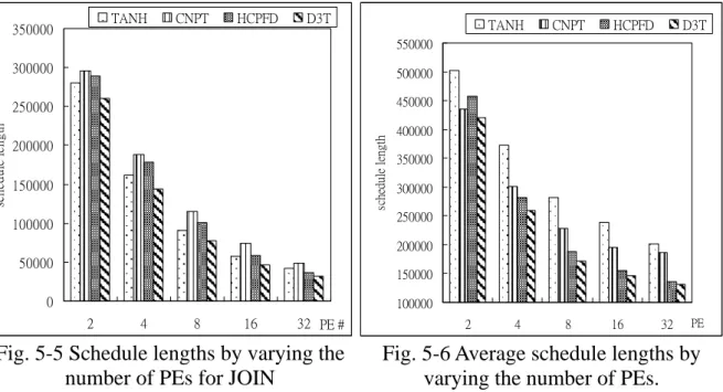
Fig. 5-5 Schedule lengths by varying the number of PEs for JOIN

100000 150000 200000 250000 300000 350000 400000 450000 500000 550000 2 4 8 16 32 sc he du le l eng th TANH CNPT HCPFD D3T PE

Fig. 5-6 Average schedule lengths by varying the number of PEs.

In Fig. 5-5, the scheduling performance of the TANH algorithm is better than that of the HCPFD and CNPT algorithms when the number of PEs is 2, 4, 8, or 16. As mentioned in chapter 2, the TANH algorithm allocates the shortest path to each cluster and the paths are generated by the bottom-up strategy. Fig. 5-5 shows that the TANH algorithm is good to aim at the join task graph. Finally, the experimental results show that the D3T algorithm is better than other algorithms and monotonically reduces the schedule length as the number of PEs increases.

As follows, Fig. 5-7~ Fig. 5-12 show the average schedule lengths by varying CCRs.

50000 70000 90000 110000 130000 150000 170000 190000 210000 230000 0.1 0.3 0.5 0.7 0.9 1 2 4 6 8 10 sc he dul e le ng th TANH CNPT HCPFD D3T CCR

Fig. 5-7 Schedule lengths by varying CCRs for FFT.

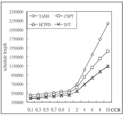
350000 550000 750000 950000 1150000 1350000 1550000 1750000 1950000 2150000 2350000 0.1 0.3 0.5 0.7 0.9 1 2 4 6 8 10 sc he dul e le ngt h TANH CNPT HCPFD D3T CCR

Fig. 5-8 Schedule lengths by varying CCRs for LU.

Fig. 5-7 and Fig. 5-8 demonstrate that the difference between the D3T and HCPFD algorithms is minor when the CCR is bigger than one.

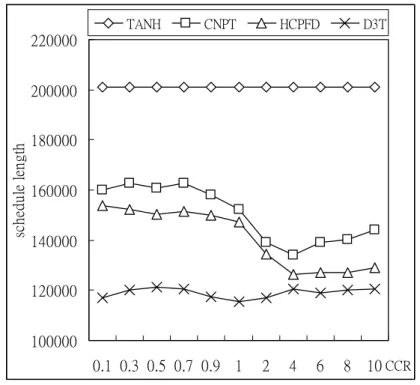
140000 150000 160000 170000 180000 190000 200000 210000 220000 0.1 0.3 0.5 0.7 0.9 1 2 4 6 8 10 sc he dul e le ngt h TANH CNPT HCPFD D3T CCR

Fig. 5-9 Schedule lengths by varying CCRs for GJE.

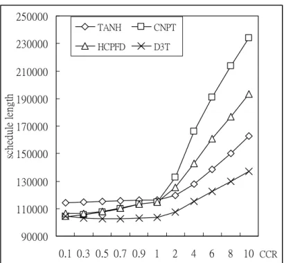
100000 120000 140000 160000 180000 200000 220000 0.1 0.3 0.5 0.7 0.9 1 2 4 6 8 10 sc he du le l en gt h TANH CNPT HCPFD D3T CCR

Fig. 5-10 Schedule lengths by varying CCRs for FORK.

As shown in Fig. 5-9 and Fig. 5-10, the average schedule length obtained by the D3T algorithm increases slightly. The experimental results of the Fig. 5-9 and Fig. 5-10 demonstrate that the D3T algorithm could get stable scheduling performance

regardless the CCRs among each machine. According to the comparison with the four algorithms presents the evident advantage of the D3T algorithm when the CCR is increasing. Besides, Fig. 5-10 shows that the average schedule lengths generated by the CNPT and HCPFD algorithm are decreasing when the CCR is bigger than 1. The main reason is that the CNPT and HCPFD algorithm do not assign the priority to the non-CN. The CNPT and HCPFD algorithm get worse scheduling performance when the CCR is smaller than 1. Therefore, Fig. 5-10 demonstrates that the order of allocating nodes to PEs affects the schedule lengths a lot. Otherwise, the average schedule lengths obtained by the TANH algorithm is also stable when the CCR are 0.1, 0.3, 0.5, 0.7, 0.9, 1, 2, 4, 6, 8, and 10. 90000 110000 130000 150000 170000 190000 210000 230000 250000 0.1 0.3 0.5 0.7 0.9 1 2 4 6 8 10 sc he dul e le ngt h TANH CNPT HCPFD D3T CCR

100000 150000 200000 250000 300000 350000 400000 450000 500000 550000 600000 0.1 0.3 0.5 0.7 0.9 1 2 4 6 8 10 sc hed ul e len gt h TANH CNPT HCPFD D3T CCR

Fig. 5-12 Average schedule lengths by varying CCRs.

Fig. 5-11 shows that the average schedule lengths generated by the TANH algorithm are smaller than that obtained by the HCPFD algorithm when the CCR is bigger than 1. The experimental results demonstrate that the D3T algorithm outperforms the other three algorithms as the CCR is increasing. Fig 5-12 shows the average schedule lengths obtained by the CNPT algorithm increase rapidly when the CCR is bigger than 4. It is reasonable that the longer average schedule lengths are caused by the communication overhead.

In the following, Fig. 5-13~ Fig. 5-18 show the average schedule lengths by the varying number of processor heterogeneities.

50000 70000 90000 110000 130000 150000 170000 190000 0.2 0.4 0.6 0.8 1 2 4 6 8 10 sc he dul e le n gt h TANH CNPT HCPFD D3T pe_var

Fig. 5-13 Schedule lengths by varying the number of pe_var for FFT.

500000 600000 700000 800000 900000 1000000 1100000 0.2 0.4 0.6 0.8 1 2 4 6 8 10 sc he dul e le ngt h TANH CNPT HCPFD D3T pe_var

Fig. 5-14 Schedule lengths by varying the number of pe_var for LU.

Fig. 5-13 and Fig. 5-14 show that the average schedule lengths obtained by the four algorithms are not stable when the number of pe_var is bigger than 2.

120000 140000 160000 180000 200000 220000 240000 0.2 0.4 0.6 0.8 1 2 4 6 8 10 sc he dul e le ngt h TANH CNPT HCPFD D3T pe_var

Fig. 5-15 Schedule lengths by varying the number of pe_var for GJE.

Fig. 5-15 shows that the average schedule lengths generated by the HCPFD and TANH algorithms are unstable when the number of pe_var is smaller than 2. As mentioned previously, the HCPFD algorithm has worse scheduling performances for performing the GJE application. Otherwise, according to the characteristic of the TANH algorithm, it would generate the same paths in each GJE task graph. It is reasonable that varying the number of pe_var affects the average schedule lengths obviously.

60000 80000 100000 120000 140000 160000 180000 200000 220000 240000 260000 0.2 0.4 0.6 0.8 1 2 4 6 8 10 sc he du le l eng th TANH CNPT HCPFD D3T pe_var

Fig. 5-16 Schedule lengths by varying the number of pe_var for FORK.

80000 90000 100000 110000 120000 130000 140000 150000 160000 170000 180000 0.2 0.4 0.6 0.8 1 2 4 6 8 10 sc he dul e le ngt h TANH CNPT HCPFD D3T pe_var

150000 200000 250000 300000 350000 400000 0.2 0.4 0.6 0.8 1 2 4 6 8 10 sc he dul e le ng th TANH CNPT HCPFD D3T pe_var

Fig. 5-18 Average schedule lengths by varying the number of pe_var.

Fig. 5-13~ Fig. 5-18 demonstrate that the average schedule lengths obtained by the four algorithms would be unstable when the number of pe_var is bigger than 2. However, the D3T algorithm outperforms the other three algorithms in terms of the average schedule length by varying the number of pe_var.

In the following, Fig. 5-19~ Fig. 5-24 show the average system utilization by varying the number of PEs.

0% 10% 20% 30% 40% 50% 60% 70% 80% 90% 2 4 8 16 32 u ti liz ati on TANH CNPT HCPFD D3T PE #

Fig. 5-19 Utilization by varying the number of PEs for FFT.

0% 10% 20% 30% 40% 50% 60% 70% 80% 90% 100% 2 4 8 16 32 ut ili za tio n TANH CNPT HCPFD D3T PE #

20% 30% 40% 50% 60% 70% 80% 90% 100% 2 4 8 16 32 uti liz at io n TANH CNPT HCPFD D3T PE #

Fig. 5-21 Utilization by varying the number of PEs for GJE.

20% 30% 40% 50% 60% 70% 80% 90% 100% 2 4 8 16 32 u ti liz ati on TANH CNPT HCPFD D3T PE #

20% 30% 40% 50% 60% 70% 80% 90% 100% 2 4 8 16 32 u til izat io n TANH CNPT HCPFD D3T PE #

Fig. 5-23 Utilization by varying the number of PEs for JOIN.

20% 30% 40% 50% 60% 70% 80% 90% 100% 2 4 8 16 32 ut ili za tio n TANH CNPT HCPFD D3T PE #

Fig. 5-24 Average utilization by varying the number of PEs.

Fig. 5-19~ Fig. 5-24 demonstrate that the average system utilization obtained by the CNPT, HCPFD, TANH, and D3T algorithms reduce monotonically as the numbers of PEs increases. It is reasonable that the system utilization reduces when the