A Hyperplane-Constrained Continuation
Method for Bound States of Coupled
Nonlinear Schr¨
odinger Equations
Yuen-Cheng Kuo
a, Wen-Wei Lin
b, Shih-Feng Shieh
c,
Weichung Wang
daDepartment of Applied Mathematics, National University of Kaohsiung,
Kaohsiung 811, Taiwan ([email protected]).
bDepartment of Mathematics, National Tsinghua University, Hsinchu 300, Taiwan
cDepartment of Mathematics, National Taiwan Normal University, Taipei 116,
Taiwan ([email protected]).
dDepartment of Mathematics, National Taiwan University, Taipei 106, Taiwan
Abstract
Time-independent m-coupled nonlinear Schr¨odinger equations (NLSEs) that can be used to model nonlinear optics are studied analytically and numerically in this article. Starting from a one-component discrete nonlinear Schr¨odinger equa-tion (DNLSE), we first propose and analyze an iterative method for finding the ground state solution. This solution is then used as the initial point of the primal stalk solution curve of the m-coupled DNLSEs in a continuation method framework. To overcome the stability and efficiency problems arising in standard continuation methods, we propose a hyperplane-constrained continuation method by adding ad-ditional constraints while following the solution curves. Furthermore, we analyze solution and bifurcation properties of the primal stalk solution curve correspond-ing to the 3-coupled DNLSEs. We also demonstrate computational positive bound states and bifurcation diagrams of the 3-coupled DNLSEs, including non-radially symmetric ground states that are tricky to find in NLSEs.
Key words: Hyperplane-constrained continuation method, m-coupled nonlinear
Schr¨odinger equations, iterative method for one-component problem, primal stalk solutions, non-radially symmetric, ground states.
1 Introduction
In this article, we consider the following time-independent m-coupled nonlin-ear Schr¨odinger equations (NLSEs),
4φj − λjφj + µj|φj|2φj+ m X i6=j,i=1 βij|φi|2φj = 0, in Rn, (1a) φj > 0 in Rn, j = 1, . . . , m, (1b) φj(z) → 0, as |z| → ∞, (1c)
where λj, µj > 0 are positive constants, n ≤ 3, and βij = βji (i 6= j) are coupling coefficients. The NLSEs model a physical phenomenon in nonlinear optics [1], where the solution φj denotes the j-th component of the beam in Kerr-like photorefractive media. The positive constant µj is for self-focusing in the j-th component of the beam; and λj is referred to as the chemical potential. The coupling constant βij is the interaction between the i-th and j-th component of j-the beam. For βij > 0, the interaction is attractive; otherwise, the interaction is repulsive.
To solve Equations (1) numerically, the corresponding m-coupled discrete non-linear Schr¨odinger equations (DNLSEs) can be written as
Auj − λjuj+ µju°j2 ◦ uj + Pm i6=j,i=1βiju°i2 ◦ uj = 0, uj > 0, uj ∈ RN, for j = 1, . . . , m, (2) where uj ∈ RN denotes the approximation of φj(z), for j = 1, . . . , m. Here A ∈ RN ×N is the standard central finite difference discretization matrix of the Laplacian operator with the homogeneous Dirichlet boundary conditions. Additionally, it can be seen that A is an irreducible and symmetric negative definite matrix. The size of N depends on the approximation domain and grid sizes. For example, if a uniform grid size h is applied on a square finite domain [−d, d] × [−d, d] for n = 2, we have N = (2d
h − 1)2. For u = (u1, . . . , uN)>, v = (v1, . . . , vN)> ∈ RN, u ◦ v = (u1v1, . . . , uNvN)> denotes the Hadamard product of u and v and u°r = u◦· · ·◦u denotes the r-time Hadamard product
of u.
We thus study the m-coupled DNLSEs by conducting numerical analysis and developing efficient numerical schemes in the framework of continuation meth-ods. However, one particular characteristic of Equations (1) posts challenges for computing the numerical solutions. Since the solution domain is unbounded in (1), a shift of any solution of the system remains a solution of the system. Consequently, a small shift of a numerical solution of an m-coupled DNLSEs (on a bounded computational domain) can also be an approximate solution of another m-coupled DNLSEs with a small residual. This phenomenon prevents
classical continuation methods from being applicable or efficient for solving the target problem. First, the prediction directions may not be unique. Second, the Jacobian matrix may be nearly singular and the corresponding Newton’s correction process become inaccurate and inefficient. Third, the numerical singularity also makes detections of bifurcation points difficult. Finally, these improper search directions may result in undesired solution curves in contin-uation methods.
To compute positive bound state solutions of m-coupled DNLSEs, this article makes the following contributions:
• We first develop a globally convergent method for computing the positive ground state solution of one-component DNLSE. This ground state solution can be used to describe the primal stalk of the solution curve of m-coupled DNLSEs.
• Aiming at 3-coupled DNLSEs, we characterize the primal stalk solutions and prove that the primal stalk of the solution curve of 3-coupled DNLSEs has at least N − p bifurcation points at finite values of coupling constants β, where N is the number of grid points and p is the number of nonnegative eigenvalues of a particular matrix.
• In order to remedy the defectiveness mentioned above, we propose a hyperplane-constrained continuation method to compute all possible positive bound states of m-coupled DNLSEs by adding additional hyperplane constraints, so that the prediction directions can be uniquely determined and the cor-rection dicor-rections can be computed efficiently.
• By using the proposed hyperplane-constrained continuation method, we conduct numerical experiments to explore versatility of numerical solutions by presenting solution profiles, bifurcation diagrams, and corresponding en-ergies for various settings.
• We further develop a continuation scheme to qualitatively find the non-radially symmetric solution predicted in [20]. This asymmetric solution cannot be obtained by following solution curves straightforwardly. The pro-posed scheme verifies the existence of the solution numerically and visually. The target problem have been considered in several cases. For n = 1, i.e. the spatial dimension is one, the system (1) is integrable. Many analytical and numerical results on solitary wave solutions of m-coupled NLSEs were well-studied in, e.g., [10,14–16]. For n = 2 and m = 1, physical experi-ments in [21] observed 2-dimensional photorefractive screening solutions and a dimensional self-trapped beam. It is natural to believe that there are 2-dimensional m-component (m ≥ 2) solitons and self-trapped beams. A general theorem for the existence of high dimensional m-component solitons is firstly proved in [20]. The sign of coupling constants βij’s is crucial for the existence of ground state solutions. For m = 3, when all βij’s are positive, there exists a ground state solution which is radially symmetric. Furthermore, a positive
bound state solution which is non-radially symmetric is also found. See [20] for details.
It is worth mentioning that if the NLSEs are equipped with trap potentials, the difficulties resulting from solution shifting no longer exist and following numerical methods can be used to solve the equations. Bao proposed a normal-ized gradient flow method [4,5] and a time-splitting sine-spectral method [4]. For time-independent case, a Gauss-Seidel-type iteration has been proposed in [9]. Furthermore, a continuation BSOR-Lanczos-Galerkin method has been developed in [8,18]. More recently, the technique of Liapunov-Schmidt reduc-tion and continuareduc-tion method have been developed in [3].
This paper is organized as follows. In Section 2, we develop an iterative method to compute the positive ground state solution of one-component DNLSE and show that the iterative method is globally convergent. In Section 3, we develop a hyperplane-constrained continuation method to compute positive bound state solutions of m-coupled DNLSEs. In Section 4, we prove the existence of the bifurcation of a 3-coupled DNLSEs at finite values of the coupling con-stant β. Numerical results of positive bound states of some 3-coupled DNLSEs systems are presented in Section 5.
1.1 Definitions and notations
We now give the definition of the ground state solution of (1) to be used in the following study. In the case of one-component (m = 1), the solution of (1) can be obtained through the minimization problem
inf φ ≥ 0 φ ∈ H1(Rn) R Rn|∇φ|2+ λ R Rnφ2 (RRnφ4)1/2 (3)
with a suitable scaling. Another equivalent formulation of (3) is to consider the following minimization problem
inf φ∈N1 E(φ) (4a) where N1 = ½ φ ∈ H1(Rn)| φ ≥ 0, φ ≡/ 0, Z Rn|∇φ| 2+ λZ Rnφ 2 = µZ Rnφ 4 ¾ (4b) and E(φ) = 1 2 Z Rn|∇φ| 2+λ 2 Z Rnφ 2− µ 4 Z Rnφ 4. (4c)
If φ solves the optimization problem defined in (4), φ is called a ground state solution. Hereafter, we extend the definition of the ground state solution to m-component cases. We define
Nm = {φ = (φ1, φ2, . . . , φm) ∈ (H1(Rn))m| φj ≥ 0, φj ≡/ 0 and Z Rn|∇φj| 2 + λ j Z Rnφ 2 j = µj Z Rnφ 4 j + m X i6=j,i=1 βij Z Rnφ 2 iφ2j, j = 1, . . . , m} (5) and the energy functional
E(φ) = m X j=1 Ã 1 2 Z Rn|∇φj| 2+λj 2 Z Rnφ 2 j − µj 4 Z Rnφ 4 j ! − 1 4 m X i, j = 1 i 6= j βij Z Rnφ 2 iφ2j, (6) where φ = (φ1, . . . , φm) ∈ (H1(Rn))m. Then, we consider the minimization problem
inf φ∈Nm
E(φ). (7)
If φ = (φ1, . . . , φm) ∈ Nm has the following properties:
(i) φj > 0 for all j and φ satisfy (1);
(ii) E(φ) ≤ E(ψ) for any other solution ψ of (1), then φ is called a ground state solution of (1).
We define the corresponding energy functional for the m-coupled DNLSEs (2) as follows. The energy functional E(φ) in (6) becomes
E(x) = m X j=1 Ã −1 2u > jAuj+ λj 2u > j uj − µj 4u °2> j u° 2 j ! − 1 4 m X i, j = 1 i 6= j βiju°i2>u° 2 j , (8)
where the vector x = (u>
1, . . . , u>m)>∈ RN m is in Nm = {(u>1, . . . , u>m)>∈ RN m| uj ≥ 0, uj ≡/ 0 and −u> j Auj+ λju>juj = µju°j2>u° 2 j + m X i6=j,i=1 βiju°i2>u° 2 j , j = 1, . . . , m}. (9) Throughout this paper, we use bold face letters or symbols to denote a matrix or a vector. For u = (u1, . . . , uN)>, [[u]] := diag(u) denotes the diagonal
matrix of u and kuk4 = (u°2>u°2)1/4. For A ∈ RN ×N, A > 0 (≥ 0) denotes
a positive (nonnegative) matrix with positive (nonnegative) entries, A Â 0 (with A> = A) denotes a symmetric positive definite matrix, σ(A) denotes the spectrum of A, and N (A) and R(A) denote the null and range spaces of A, respectively.
2 Iterative method for one-component DNLSE
To solve the m-coupled NLSEs (1) numerically, we adopt the framework of continuation methods (e.g. [2,17]) by varying βij’s. We start the discussion of numerical schemes and the corresponding analyses for solving the m-coupled DNLSEs from the simplest case of m = 1, which can be viewed as the de-coupled equation in which all βij’s are equal to zero. An iterative method is developed and analyzed for computing the ground state solution of this one-component DNLSE. Furthermore, the solution is then used as the initial solution of the primal stalk solution curve of the m-coupled DNLSEs.
The one-component DNLSE is described by Au − λu + µu°2 ◦ u = 0, u > 0, uj ∈ RN, (10) where λ and µ are positive constants. The discretization of the minimization problem (3) can be formulated by
inf u≥0 b E(u), (11a) where b
E(u) = −u>Au + λu>u
(u°2>u°2 )1/2 . (11b)
From (4), the equivalent formulation of (11) becomes inf u∈N1 E(u), (12a) where E(u) = −1 2 u >Au + λ 2u >u − µ 4u °2>u°2 (12b) and N1 = n
[Fixed Point Iteration] (i) Let ¯A ∈ RN ×N, u
0 > 0 with ku0k4 = 1, and i = 0;
(ii) Solve the linear system
¯
Aui+1= u°i3. Compute ui+1 = ui+1/kui+1k4.
(iii) If convergence, then u∗ ← u
i+1, stop; else i ← i + 1, go to (ii).
It is easily seen that any solution u ∈ RN of (10) is a local minimum or a saddle point of (12).
Next we develop a numerical algorithm for finding the global minimum of (12), i.e., the ground state solution of the one-component DNLSE (10). The ma-trix A in (10) is generically diagonal dominant with nonnegative off-diagonal entries. That is, −A is an irreducible M-matrix. Let
¯
A = λI − A. (13)
Then ¯A is an irreducible M-matrix because λ > 0. It follows that ¯A−1 is positive definite with positive entries (i.e., ¯A−1 Â 0 and ¯A−1 > 0). We define the set M =nu ∈ RN| kuk 4 = 1, u ≥ 0 o , ◦
M =nu ∈ RN| u belongs to the interior of Mo. (14) It is easy to verify that if u ∈ M, then
¯
A−1u = (λI − A)−1u > 0. (15)
We now define a map f : M → M by
f(u) = A¯−1u°
3
k ¯A−1u°3 k 4
. (16)
Since the map f is well-defined by (15) and (16), we can use f to define the fixed point iteration ui+1= f(ui) as the following algorithm.
2.1 Analysis of the iterative algorithm
In this section, we analyze the convergence behavior of Algorithm 2. First, we show that the map f has a fixed point and then we build up the connection between the fixed point and the one-component DNLSE.
Furthermore, the vector ¯ u(µ) = 1 µ1/2k ¯A −1u∗°3 k−1/2 4 u∗ ∈ N1 (17)
solves the one-component DNLSE (10).
Proof. Equations (15) and (16) imply that f is continuous on M. By the definition of (14), M is homeomorphic to an (N − 1)-dimensional standard simplex which is convex and compact. Applying the Schauder fixed point theorem to f, we can see that there is a point u∗ ∈ M satisfying
f(u∗) = u∗. (18)
The fixed point u∗ ∈M follows from the fact that the function f in (16) maps◦
M into M. From (13), (16) and (18), we have◦
k ¯A−1u∗°3 k−1
4 u∗°3 = (λI − A)u∗. (19)
Multiplying (19) by 1
µ1/2k ¯A−1u∗° 3k−1/2
4 from the left and setting
¯ u(µ) = 1 µ1/2k ¯A −1u∗°3 k−1/2 4 u∗, we obtain
A¯u(µ) − λ¯u(µ) + µ¯u(µ)°3 = 0.
It is easy to verify that ¯u(µ) belongs to N1. This completes the proof. 2
Theorem 1 suggests that the one-component DNLSE (10) has a solution ¯u(µ) that can be computed by using the fixed point of f. Furthermore, since the one component NLSE (1) has a unique solution [19], the solution ¯u(µ) is expected to be the unique (and thus the ground state) solution of the one-component DNLSE (10), although a strict proof is absent.
We have suggested solving the one-component DNLSE (10) by Algorithm 2. The following theorems further discuss how the solution sequence generated by Algorithm 2 converges to a fixed point of f. In Theorem 2 below, we first show that the energy sequence corresponding to the iterates is decreasing and therefore a subsequence of the iterates converges to a fixed point in M of f. In Theorem 3 below, by making a mild assumption, we further show that the whole sequence {ui}∞i=0 generated by Algorithm 2 converges to u∗ ∈ M globally.
Theorem 2 (i) If u ∈ M and v = f(u), then E(v) ≤b E(u), whereb E(·)b is defined in (11b). The equality holds if and only if u is a fixed point of
f : M → M, i.e., f(u) = u.
(ii) For a sequence {ui}∞i=0generated by Algorithm 2, there exists a subsequence
{uni}∞i=0 such that
lim
i→∞uni = u
∗, (20)
where u∗ ∈ M is a fixed point of the function f defined in (16).
Proof. (i) Since u, v ∈ M, we have kuk4 = 1, kvk4 = 1 and
b
E(v) = v>(λI − A)v. (21)
Substituting v = f(u) = A¯ −1u°3 k ¯A−1u°3k 4 into (21), we get b
E(v) = v>(λI − A)v = 1
k ¯A−1u°3 k 4
v>u°3.
Letting c = 1
k ¯A−1u°3k4 and applying the H¨older inequality (|x>y| ≤ kxkpkykq
where 1
p + 1q = 1 and p > 1) with p = 4, q = 4/3, x = v and y = u°
3 , we
obtain
v>(λI − A)v ≤ ckvk
4kuk34 = c. (22)
Since kuk4 = 1, we have
c = u>A ¯¯A−1u° 3
k ¯A−1u°3 k 4
= u>(λI − A)v. (23)
Since λI − A is positive definite, it has the Cholesky factorization (λI − A) = L>L. Applying the Cauchy-Schwarz inequality to (23), we obtain
c = u>L>Lv ≤√u>L>Lu ·√v>L>Lv =
q
u>(λI − A)u ·qv>(λI − A)v. (24) From (22) and (24), it follows that
v>(λI − A)v ≤ c ≤qu>(λI − A)u ·qv>(λI − A)v (25) and therefore
q
v>(λI − A)v ≤qu>(λI − A)u. Using the fact that kvk4 = kuk4 = 1, we have
b E(v) = v >(λI − A)v kvk2 4 ≤ u >(λI − A)u kuk2 4 =E(u).b (26)
The equality in (26) holds if and only if the H¨older and Cauchy-Schwarz inequalities in (22) and (23), respectively, become equalities. Furthermore, both inequalities hold if and only if the vectors v and u are linearly dependent, i.e., v = au for some a ∈ R. Since v > 0, u > 0 with kvk4 = kuk4 = 1, we
have v = u. Hence, the equality in (26) holds if and only if u is a fixed point of f.
(ii) Since the sequence {ui}∞i=0 ⊂ M is bounded, there exists a convergent subsequence {uni}
∞
i=0 and a u∗ ∈ M such that lim i→∞uni = u ∗. Consequently, we have lim i→∞ b E(uni) =E(ub ∗) and lim i→∞ b E(f(uni)) =E(f(ub ∗)), (27)
as f andE are continuous. Furthermore, since the cost functionb E(·) in (11b)b is continuous on the compact set M, the function E(·) : M → Rb + attains
its minimum value on M. From part (i) of this theorem, it can be easily seen that the sequence {E(ub i)}∞i=1converges to a certain positive numberEb∗. That is,
lim i→∞
b
E(ui) = Eb∗. (28)
By Equations (27), (28), and the fact that {E(ub ni)}∞i=0 and {E(f(ub ni))}∞i=0
are subsequences of {E(ub i)}∞i=0, we see that the three sequences converge to the same value. Consequently, we have
b
E(f(u∗)) =E(ub ∗). By part (i) of this theorem, we conclude that
f(u∗) = u∗.
2
The following corollary can be easily obtained by applying Theorem 2. Theorem 1 If the minimization problem (11) has a unique global minimizer u∗ ∈ M, then there exists a neighborhood R
u∗ of u∗ such that the fixed point
iteration converges to u∗ for any initial vector u
0 ∈ Ru∗. In addition, ¯u(µ),
defined in (17), is a global minimizer of (12).
We have proved that there is a subsequence converging to a fixed point. Now we discuss how Algorithm 2 converges entirely. To do so, we first define the
¯
A-norm of u by kukA¯ =
√
u>Au and introduce the following lemma. Note¯ that the definition of ¯A-norm is well-defined as ¯A is positive definite.
Theorem 1 Let {ui}∞i=0 be the sequence generated by Algorithm 2. We have lim
i→∞kui+1− uikA¯ = 0. (29)
Proof. By definition,
kui+1− uik2A¯ = (ui+1− ui)>A(u¯ i+1− ui) = u>
i+1Au¯ i+1+ u>i Au¯ i− 2u>i+1Au¯ i
=E(ub i+1) +E(ub i) − 2u>i+1Au¯ i. (30) From (22), (23) and (25), we have
b
E(ui+1) ≤ u>i+1Au¯ i ≤ q b E(ui+1) q b E(ui). (31) Furthermore, by (30) and (31), it follows that
kui+1− uikA¯ ≤
q b
E(ui) −E(ub i+1), (32) or equivalently, limi→∞kui+1− uikA¯ = 0. 2
Theorem 3 (Existence of globally convergent sequence) If u∗given in (20) is a strictly local minimum of (11), then the sequence {ui}∞i=0 generated
by Algorithm 2 converges to u∗ ∈ M.
Proof. Since u∗ is a strictly local minimum of the optimization problem (11), the Hessian matrix H(u∗) of E(u) is positive definite. Therefore, there is ab δ > 0 such that H(u) is positive definite, i.e.,E(u) is convex, for u ∈ M andb ku − u∗k
¯ A < δ.
For any positive number 0 < ε < δ/2, we let b Eε= min ku−u∗k¯ A=ε b E(u) >Eb∗, (33)
where Eb∗ is given by (28), and define
B(u∗,Eb ε) = n u ∈ M¯¯¯ku − u∗k ¯ A < ε, E(u) <b Ebε o . (34) From (20) and (29), there exists N0 ∈ N such that
unj ∈ B(u
∗,Eb
ε) and kui+1− uikA¯ < ε for nj, i > N0. (35)
Since 2ε < δ, if ui ∈ B(u∗,Ebε) and kui+1− uikA¯ < ε, then kui+1− u∗kA¯ < 2ε.
On the other hand, using the fact that E(ub i+1) ≤ E(ub i) < Ebε and E(u) isb convex on ku − u∗k¯
A < δ it holds that ui+1∈ B(u∗,Ebε). Thus, we have
This completes the proof. 2
In Theorem 3, we have shown that if a limit point u∗ of {u
i}∞i=0 is a strictly local minimum of (11), then {ui}∞i=0generated by Algorithm 2 converges glob-ally to u∗ ∈M and u◦ ∗ satisfies
(λI − A)u∗ = τ u∗°3 where τ = k ¯A−1u∗°3k
4. (36)
We can then compute ¯u(µ) by (17) to find the ground state solution of the one-component DNLSE (10). Although the assumption of a strictly local min-imum is needed to prove the global convergence in Theorem 3, numerical experience shows that the fixed point iteration (Algorithm 2) converges glob-ally to the global minimizer of (11) for any arbitrary initial positive vector u0
with ku0k4 = 1.
3 Hyperplane-constrained continuation method for the DNLSEs In this section, we develop a hyperplane-constrained continuation method to solve the m-coupled DNLSEs (2). We assume the variable βij is changeable and introduce the continuation method parameter β ≥ 0 into Equation (2) by rewriting
βij = δijβ (37)
for i, j = 1, . . . , m and i 6= j. Here δij’s are nonzero constants and δij = δji. If
δij > 0, the interaction between the i-th and the j-th components is attractive; if δij < 0, the interaction is repulsive. Furthermore, to fit the framework of a continuation method better, we rewrite the m-coupled DNLSEs (2) as
G(x, β) = 0, (38a)
where x = (u>
1, . . . , u>m)> ∈ RN m and G = (G1, . . . , Gm) : RN m× R → RN m is a smooth mapping with
Gj(x, β) = Auj− λjuj + µju°j2 ◦ uj+ β m X i6=j,i=1 δiju°i2 ◦ uj, j = 1, . . . , m. (38b) We let DG denote the Jacobian matrix of G; in particular,
DG = [Gx, Gβ] ∈ RM ×(M +1), where M = Nm. We define the solution curve of (2) as
Here we assume a parametrization via arc-length s is available on C. By dif-ferentiating Equation (38) with respect to s, we obtain
DG(y(s)) ˙y(s) = 0, (40) where ˙y(s) = ( ˙x(s)>, ˙β(s))> is a tangent vector of C at y(s).
Equation (40) suggests that the tangent vector to C at y(s) is the natural nontrivial solution of the M × (M + 1) homogeneous system DG(y(s))w = 0, when DG(y(s)) is of full row rank. However, if DG(y(s)) is not of full rank at a certain s, then the the continuation algorithm is not well-defined. In this case, typical continuation methods may not follow the solution curve successfully. The motivation of our hyperplane-constrained continuation method can be straightforwardly illustrated from the observation on the NLSEs for n = 1. Based on the observation, we then return to the DNLSEs for n = 2. Afterward we discuss how we may circumvent the obstacle for general cases in Section 3.1. Considering the 2-coupled NLSEs (1) with n = 1 and a fixed β12, we
differen-tiate sides of (1a) with respect to x and obtain
Gx(y(s)) φ 0 1 φ02 = L1 2β12φ1φ2 2β12φ1φ2 L2 φ 0 1 φ02 = 0, (41) where L1 = d 2 dx2 − λ1 + 3µ1φ21 + β12φ22 and L2 = d 2 dx2 − λ2 + 3µ2φ22 + β12φ21.
Equation (41) implies that the matrix Gx(y(s)) is actually singular with the
corresponding singular vector [ φ0
1, φ
0
2]>. Furthermore, there exists a one
di-mensional solution set of (1) for a fixed β12
{φr(x)|φr(x) = (φ1(x − r), φ2(x − r)), r ∈ R} (42)
that contains all the translation solutions. These characters post the following two difficulties that may be encountered by a standard continuation method. First, the singularity may cause accuracy and efficiency problems while solving the resulting linear system. Second, a continuation method may be trapped or hard to keep moving ahead due to the translation solutions described in (42). Similar problems can be observed in the m-coupled DNLSEs (2) with n = 2. We consider a bounded domain [−d, d]×[−d, d], where the size d is sufficiently
large and the uniform grid size h is sufficiently small. Let D = 1 2h 0 1 0 −1 . .. ... . .. ... 1 0 −1 0 ∈ R√N ×√N
be the central difference operator. We define c
Dx = D>⊗ I√N, cDy = I√N ⊗ D ∈ RN ×N
as the discretization matrices of the differential operators ∂
∂x and ∂y∂, respec-tively. Then one can check that, similar to the operator d
dx in (41),
K0 = span{Dxx(s), Dyx(s)} (43)
forms a numerical null space of Gx(x(s), β(s)), where
Dx = diag{cDx, . . . ,cDx}, Dy = diag{cDy, . . . ,cDy} ∈ RN m×N m. (44) In practice, if we use p ≡ a[(Dxx(s))>, 0]>+ b[(Dyx(s))>, 0]> (a2+ b2 = 1) as the prediction direction, then, numerically, the “new solution” x(˜s) (˜s ≈ s) computed by the continuation method is a small shift of x(s) in the p-direction. These new solutions generally have very small residual kG(x(s), β(s))k < ε and are called “ε-solutions”. Since the domain of (2) is bounded, the residual gets larger if we keep shifting x(s) along the p-direction, where (x(s), β(s)) is the solution of G(y(s)) = 0. These ε-solutions further result in the following challenges to the prediction-correction scheme of the continuation method.
(1) In the prediction step, we cannot compute a unique prediction direction by solving (40).
(2) In the correction step, since the Jacobian matrix Gx is nearly singular,
Newton’s correction will lose quadratic convergence and its accuracy. (3) The numerical singularity of the Jacobian matrix can make detections of
bifurcation points difficult.
(4) Since the solution manifold C in (39) contains a 2-dimensional ε-solution set and the “good” prediction direction is not unique, the solutions com-puted by the continuation method may appear to be random or trapped in the ε-solution set. That is, we can not follow the desired solution curve C in (39) efficiently by the continuation method.
To overcome these difficulties, we develop a hyperplane-constrained continua-tion method for solving (38) in the following subseccontinua-tions.
3.1 Prediction and correction
Let yi = (x>i , βi)> ∈ RM +1 be a point that has been accepted as an ap-proximation point for the solution curve C. A “good” prediction direction ˙yi = ( ˙x>i , ˙βi)> should satisfy (40) and the vector ˙x>i should be in K0⊥, where
K0 is given in (43). It follows that the prediction direction ˙yi ∈ RM +1 should satisfy the bordered linear system
Gx Gβ a> x 0 a> y 0 c> i ci ˙yi = 0 0 0 1 , (45)
where ax = Dxxi, ay = Dyxi, and (c>i , ci)> ∈ RM +1 is a suitable constant vector. Note that Equation (45) can be interpreted geometrically as follows. The next solution yi+1 must pass through the two hyperplanes whose normal vectors are ax and ay. In other word, we first use the Euler predictor
yi+1,1 = yi+ hi˙yi
to predict a new point yi+1,1, where hi > 0 is the step length and ˙yi is the unit tangent vector at yi that is obtained by normalizing the solution of the bordered linear system (45).
Now the solution curve C is determined by the underlying system of equations G(x, β) = 0, a> xx = 0, a> yx = 0, ˙x> i x + ˙βiβ = 0.
Starting from the predictor, the accuracy of the approximation yi+1,1 to the solution curve C can be improved by a correction process. Typically, Newton’s method is chosen as a corrector. By setting yi+1,l+1 = yi+1,l+δlfor l = 1, 2, . . ., we solve the bordered linear system
Gx(yi+1,l) Gβ(yi+1,l) a> x 0 a> y 0 ˙x> i ˙βi δl= − G(yi+1,l) ρx,l ρy,l ρl , (46)
[Mixed Block Elimination]. (i) Solve ξ>B = g>, (ii) Compute δ1 = γ − ξ>f, σ = (ρ − ξ>q)/δ1, (iii) Solve Bv = f, (iv) Compute δ = γ − g>v, q 1 = q − fσ, ρ1 = ρ − γσ, (v) Solve Bw = q1, (vi) Compute σ1 = (ρ1− ξ>w)/δ, (vii) Compute x = w − vσ1, σ = σ + σ1.
with ρx,l = a>xxi+1,l, ρy,l = a>yxi+1,l, and ρl = ˙y>i yi+1,l. If {yi+1,l} converges until l = l∞, then we accept yi+1 = yi+1,l∞ as a new approximation to the
solution curve C.
The two linear systems (45) and (46) are overdetermined systems and can be solved by least squares method with very small minimal residual. Another efficient way to solve (45) and (46) is to rewrite them in the form
B f g> γ x σ = q ρ , x(M + 1) = x(M + 2) = 0, (47) where B = Gx ax ay a> x 0 0 a> y 0 0 ∈ R(M +2)×(M +2) (48)
is symmetric and f, g, q ∈ R(M +2). The linear system (47) can be easily solved
by the well-known block elimination (BE) algorithm (see e.g. [17]) when B is well-conditioned. However, near turning points or branch points, B in (47) be-comes nearly singular, i.e., B is ill-conditioned. Then the linear system should be solved by the deflated block elimination (DBE) algorithm by Chan [7], or the more efficient, backward stable, mixed block elimination (BEM) algorithm proposed by Govaerts [12,11] as shown below.
Remarks. (i) The main step in Algorithm 3.1 is to solve the linear system of the form Bξ = g.
(ii) Since linear systems (45) and (46) have very small minimal residuals, Equa-tion (47) is nearly consistent. Thus, the soluEqua-tion x solved by Algorithm 3.1 satisfies x(M + 1) ≈ x(M + 2) ≈ 0 automatically.
3.2 Testing for Bifurcation
Let C be the solution curve defined in (39), y(s) ∈ C and
J(s) = Gx(y(s)) Gβ(y(s)) a> x 0 a> y 0 ∈ R(M +2)×(M +1), (49a) J(s) = Gx(y(s)) a> x a> y ∈ R(M +2)×M. (49b)
As described in [2,13,17], a point y(s) ∈ C is said to be a regular point if rank(J(s)) = M (i.e., dim N (J(s)) = 1) and is a singular point if rank(J(s)) ≤ M − 1 (i.e., dim N (J(s)) ≥ 2). For a regular point y(s), the tangent vector
˙y(s) is uniquely determined by the linear system (45).
Now our task is to design algorithms to detect singular points of the solu-tion curve C and to compute tangent vectors if y(s) is a singular point. For simplicity, here we only consider the case
[Gβ(y(s))>, 0, 0]>∈ R(J(s)) for each singular points y(s) ∈ C, (50)
i.e., dim N (J(s)) = dim N (J(s)) − 1 and dim N (J(s)) ≥ 2. This case shows that the tangent vector at a singular point has a nonzero component at ˙β(s) and can be expected to appear in the solution curve C of (38). We denote B(s) as the matrix B given by (47) at the point y(s) ∈ C.
Based on the method of [17, p.88-99], we first propose Algorithm 3.2 for find-ing the tangent vectors at sfind-ingularity.
Algorithm 3.2 Tangent Vectors at Singularity. (I) For dimN (J(s∗)) = 1 :
(i) Compute the unit right null vector φ = ( ¯φ>, 0, 0)> of B(s∗), and solve J(s∗) ¯φ
0 = −[Gβ(s∗)>, 0, 0]> with ¯φ>φ¯0 = 0, by using sparse
SVDPACK [6] (or another suitable package); (ii) Form φ1 = ¯ φ 0 and φ2 = ¯ φ0 1 ;
(iii) Solve the real vector roots {(ˆµk, ˆνk)}2k=1 of a11µ2 + 2a12µν + a22ν2
with
a11= ¯φ>Gxx(s∗) ¯φ ¯φ, a12= ¯φ>[Gxx(s∗) ¯φ0+ Gxβ] ¯φ,
a22 = ¯φ>[Gxx(s∗) ¯φ0φ¯0+ 2Gxβ(s∗) ¯φ0+ Gββ(s∗)];
(iv) Form tangent vectors ˙yk(s∗) = ˆµkφ1+ ˆνkφ2, k = 1, 2.
(II) For dimN (J(s∗)) = ` ≥ 2:
(i) Compute the unit right null vectors φ(1), . . . , φ(`)of B(s∗) with φ(k) =
( ¯φ(k)>, 0, 0)>, k = 1, . . . , ` and solve J(s∗) ¯φ
0 = −[Gβ(s∗)>, 0, 0]> with ¯φ(k)>φ¯0 = 0, k = 1, . . . , `, by using sparse SVDPACK [6] (or another suitable package);
(ii) Form φk = ¯ φ(k) 0 , k = 1, . . . , ` and φ`+1 = ¯ φ0 1 ;
(iii) Form trial tangent vectors ˙yk(s∗) = φk, k = 1, . . . , ` and ˙y`+1(s∗) =
φ`+1.
It is worth noting that detecting the singular point of the solution curve C is equivalent to finding the null vector of symmetric matrix B in (47) by the following theorem.
Theorem 4 If the condition (50) holds, then the following statements are equivalent: (i) rank(J(s)) ≤ M − 1, (ii) N (J(s)) 6= {0}, (iii) B(s) is singular and there is a nonzero vector z ∈ RM such that [z>, 0, 0]> ∈ N (B(s)).
Algorithm 3.3 Inverse Power Method. (i) Given a unit vector ζ0 ∈ R(M +2) and l = 1,
(ii) Repeat l: until convergence,
Solve Bζbl = ζl−1, where B is given in (48). Set ζl=ζbl/kζblk2, µ(l)= ζ>l Bζl;
(iii) If convergence, then µ(s) ← µ(l); else l ← l + 1, go to (ii).
Now we describe how we detect singularity of C. Let s1 < s2 be two
consec-utive continuation method parameters and µ(s1) and µ(s2) be the smallest
eigenvalues in modulus of B(s1) and B(s2), respectively. It is clear that if
µ(s1) > 0 and µ(s2) < 0, then there is a s∗ ∈ (s1, s2) such that B(s∗) is
sin-gular. We use the secant method to refine the interval (s1, s2). In the secant
method loop, we use the inverse power method (Algorithm 3.3) to compute the smallest eigenvalues. After convergence, we use Algorithm 3.2 to compute the tangent vectors at the singularity. To conclude this section, the following
algorithm summarizes how we detect the singular point s∗ of C.
Algorithm 3.4 Detection of Singularity of C.
(i) Given µ(si) the smallest eigenvalue in modulus of B(si), i = 1, 2, where
µ(s1) > 0, µ(s2) < 0, e.g., |µ(s1)| ≈ |µ(s2)| ≈ 10−4.
(ii) Do Secant Method: until convergence, (a) Compute y1(s0) := y(s0) = y(s1) +
tµ(s1)
µ(s2) − µ(s1)
, where t = y(s1) − y(s2),
(b) Perform Newton Correction (46): until convergence (i.e., ` = `∞), Solve Gx(y`(s0)) Gβ(y`(s0)) a> x 0 a> y 0 t> δ` = −G(y`(s0)) ρx,` ρy,` ρ` with ρ` = t>(y`(s0) − y1(s0)), set y`+1(s0) = y`(s0) + δ`, ` ← ` + 1, Go to (b).
(c) Compute µ(s0) of B(s0) with y(s0) = y`∞(s0) using Algorithm 3.2,
(d) If |µ(s0)| <Tol, then perform (iii)
(e) If µ(s0) > 0, s1 ← s0, else s2 ← s0, go to (ii);
(iii) Use Algorithm 3.2 to compute the desired tangent vectors with y(s∗) = y
`∞(s0).
We have proposed a continuation method for solving general m-coupled DNLSEs. In the next sections, we focus on the 3-coupled cases in both theoretical and numerical aspects. The results not only characterize the solutions of DNLSEs analytically, but demonstrate the bifurcation diagrams and visualize the the-oretical predictions in Sections 4 and [20]
4 The 3-coupled discrete nonlinear Schr¨odinger equations
Aiming at the 3-coupled discrete nonlinear Schr¨odinger equations, we first theoretically determine the primal stalk solution curve and then conduct a bifurcation analysis in this section.
solutions in [20]. Denoting βij = δijβ (see (37)) and letting Σ = 1 |β12| |β13| |β12| 1 |β23| |β13| |β23| 1 ,
some of their results regarding the 3-coupled NLSEs are categorized as follows. Case 1 (all interactions are repulsive). If δ12 < 0, δ13 < 0 and δ23 < 0,
then the ground state solution does not exist.
Case 2 (all interactions are attractive). If δ12 > 0, δ13 > 0, δ23 > 0 and
Σ is positive definite, then the ground state solution exists.
Case 3 (two repulsive and one attractive interactions). If δ12< 0, δ13 <
0, δ23 > 0 and Σ is positive definite, then the ground state solution does
not exist.
Case 4 (two attractive and one repulsive interactions). If δ12> 0, δ13 >
0, δ23< 0, β ¿ 1 and the ground state solution exists, then it must be
non-radially symmetric.
Now we use the same categories of δij’s and consider the solution curve C of (2) by letting
m = 3 and λ1 = λ2 = λ3 = µ1 = µ2 = µ3 = 1.
In such a case, the 3-coupled DNLSEs in (38) becomes
Au1− u1+ u°13 + βδ12u2°2u1+ βδ13u°32u1 = 0, (51a)
Au2− u2+ u°23 + βδ12u1°2u2+ βδ23u°32u2 = 0, (51b)
Au3− u3+ u°33 + βδ13u1°2u3+ βδ23u°22u3 = 0. (51c)
As Cases 1 and 2 are straightforward, we focus on the following two particular settings of Cases 3 and 4:
δ12 = δ13 = −1, δ23 = 1, (52a)
δ12 = δ13 = 1, δ23 = −1. (52b)
In (52a), the 3-coupled DNLSEs of (38) becomes
Au1− u1+ u°13 − βu2°2u1− βu°32u1 = 0, (53a)
Au2− u2+ u°23 − βu° 2 1 u2+ βu°32u2 = 0, (53b) Au3− u3+ u°33 − βu° 2 1 u3+ βu°22u3 = 0, (53c)
where β > 0. It is clear that if we set β := −β, then (53) describes the 3-coupled DNLSEs for the case (52b). Therefore, to investigate these two cases, we only need to consider 3-coupled DNLSEs (53) for β ∈ R.
In the following two theorems, we first explicitly determine the solutions lo-cated on the primal stalk and then discuss how other solution curves bifurcate from the primal stalk.
Theorem 5 The primal stalk of the solution curve
C = {y(s) = (x>(s), β(s))>| G(y(s)) = 0 is given in (53) and s ∈ R}, (54)
for −1
3 ≤ β < 1, has the forms
u1 = Ãs 1 + 3β 1 + β − 2β2 ! u∗ and u2 = u3 = Ãs 1 + β 1 + β − 2β2 ! u∗, (55) where x(s) = (u> 1(s), u>2(s), u>3(s))> and u∗ is given by (61). Proof. By letting u2 = u3 = κu1 with κ > 0, (56)
it follows that equations (53b) and (53c) are identical. Thus, equations in (53) can be reduced to Au1− u1+ (1 − 2βκ2)u°13 = 0, Au1− u1+ (κ2− β + βκ2)u°13 = 0. (57)
From Theorem 1, equations in (57) have a positive solution u1, if 1 − 2βκ2 =
κ2− β + βκ2. This implies that
κ = s
1 + β
1 + 3β. (58)
Substituting κ in (58) into the first equation of (57) we have Au1− u1+ 1 + β − 2β
2
1 + 3β u °3
1 = 0. (59)
It can be easily verified that if u∗ is a solution of Au − u + u°3 = 0, then
u1 =
s
1 + 3β
1 + β − 2β2u∗ ≡ ηu∗ (60)
solves (59). By Theorem 1, u∗ is given by
u∗ ≡ ¯u(1) = k ¯A−1u∗°3 k−1/24 u∗, (61)
The applicable range of β is determined by the following facts. Since κ →q1 2
as β → 1− (by (58)), we have
u2 = u3 = κu1 → ∞ (62)
by (56) and (60). On the other hand, since u1 → 0 as β → − 1 3 − (63) (by (60)), we have u2 = u3 → s 3 2u∗ by (53b) and (53c). 2
Theorem 6 The primal stalk described by (55) undergoes at least N − p bi-furcation points at finite values 0 < β = β∗
q < 1, q = 1, . . . , N − p, where p is
the number of nonnegative eigenvalues of A − I + 3[[u°2
∗ ]].
Proof. Since (53) has a positive solution curve u2(β) = u3(β) = κu1(β), for
0 < β < 1, where κ is defined in (58), the Jacobian matrix of (53) with respect to u is of the form Gu(y(β)) = B1 E1 E1 E1 B2 E2 E1 E2 B2 (64) where B1 = A − I + [[3u°12 − 2βu° 2 2 ]], (65a) B2 = A − I + [[(3 + β)u°22 − βu° 2 1 ]], (65b) E1 = −2β[[u1◦ u2]], (65c) E2 = 2β[[u°22]]. (65d)
From (56), (58) and (60), we have
u2 = u3 = s 1 + β 1 + 3βu1 = s 1 + β 1 + β − 2β2u∗, (66)
where u∗ is given by (61). Substituting (60) and (66) into (65), we get B1 = A − I + 3 + 7β − 2β 2 1 + β − 2β2 [[u °2 ∗ ]], (67a) B2 = A − I + 3 + 3β − 2β2 1 + β − 2β2 [[u °2 ∗ ]], (67b) E1 = −2β q (1 + β)(1 + 3β) 1 + β − 2β2 [[u °2 ∗ ]], (67c) E2 = 2β + 2β2 1 + β − 2β2[[u °2 ∗ ]]. (67d) Let Q = I 0 0 0 I I 0 0 I . Then QGu(y(β))Q−1 = B1 E1 0 2E1 B2+ E2 0 E1 E2 B2− E2 . (68) Hence σ(Gu(y(β))) = σ B1 E1 2E1 B2+ E2 ∪ σ(B2− E2). (69)
On the other hand, B1 E1 2E1 B2+ E2 = B1 0 0 B1 − 2β 0 κη 2[[u°2 ∗ ]] 2κη2[[u°2 ∗ ]] 2β+11 [[u° 2 ∗ ]] = 1 0 0 1 ⊗ B1− 0 1 2 1 (2β+1)κη2 ⊗ 2βκη2[[u°∗2]] = 1 0 0 1 ⊗ B1− 0 1 2 a ⊗ 2βκη2[[u°∗2]] (70)
where κ and η are given by (58) and (60), respectively, and a = 1
(2β + 1)κη2 =
1 − β q
Since a+√a2+8 2 and a− √ a2+8 2 are eigenvalues of 0 1 2 a , from (67), (69), and (70), it follows that σ(Gu(y(β))) = Λ1(β) ∪ Λ2(β) ∪ Λ3(β), (72) where Λ1(β) = σ Ã A − I + 4β + 3 2β + 1[[u °2 ∗ ]] ! , (73a) Λ2(β) = σ Ã A − I + " 3 + 7β − 2β2 1 + β − 2β2 − (a + √ a2+ 8)βκη2 # [[u°2 ∗ ]] ! , (73b) Λ3(β) = σ Ã A − I + " 3 + 7β − 2β2 1 + β − 2β2 − (a − √ a2+ 8)βκη2 # [[u°2 ∗ ]] ! . (73c) Since (a +√a2+ 8)βκη2 = (a + √ a2+ 8)βq(1 + β)(1 + 3β) 1 + β − 2β2 = β(1 − β) + β q (1 − β)2+ 8(1 + 3β)(1 + β) 1 + β − 2β2 = 4β 2 + 4β 1 + β − 2β2 = −3 + 3 + 7β − 2β2 1 + β − 2β2 , it holds that Λ2(β) = σ(A − I + 3[[u°∗2]]). (74) Hence σ(Gu(y(β)))|β=0 = Λ1(0) ∪ Λ2(0) ∪ Λ3(0) = σ(A − I + 3[[u°2
∗ ]]) ∪ σ(A − I + 3[[u°∗2]]) ∪ σ(A − I + 3[[u°∗2 ]]). (75) As β → 1−, we have that Λ1(β) → σ(A − I + 7 3[[u °2 ∗ ]]) (76) and 3+7β−2β1+β−2β22 − (a − √
a2+ 8)βκη2 → ∞. So there exists a β∗ with 0 < β∗ < 1 such that
If the number of nonnegative eigenvalues of Λ3(0) = σ(A − I + 3[[u°∗2 ]]) is p, then from (74)-(77) we see that the primal stalk of the solution curve C of (54) undergoes at least N − p bifurcation points at finite values 0 < β∗
q < 1,
q = 1, . . . , N − p. 2
5 Numerical results
In this section we study numerical results of positive bound state solutions for 3-coupled DNLSEs (51) with λ1 = λ2 = λ3 = µ1 = µ2 = µ3 = 1 by using
the hyperplane-constrained continuation method developed in Section 3. The initial point on the primal stalk of the solution curve C of (51) (i.e., the ground state solution of the one-component DNLSE) is computed by the fixed point iteration method described in Algorithm 2.
The results are summarized in the following three simulations. In Simulation 1, we assume that one attractive and two repulsive interactions occur among the components. This setting corresponds to Case 3 in Section 4. In Simula-tions 2 and 3, we assume that one repulsive and two attractive interacSimula-tions occur among the components (i.e. Case 4 in Section 4). The results in these three simulations demonstrate the versatility of the numerical solutions that can not be obtained by analytical methods. Specifically, in Simulations 1 and 2, we present the solution profiles, bifurcation diagrams, and corresponding energies for the particular settings. In Simulation 3, we develop a scheme to find the non-radially symmetric solution that is predicted in [20] qualitatively. This asymmetric solution cannot be obtained by following solution curves straightforwardly in the continuation method. The proposed scheme verifies the existence of the solution numerically and visually.
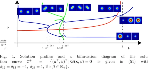
0.237 0.253 0.385 0.387 β v 1 PSfrag replacements R3N β
Fig. 1. Solution profiles and a bifurcation diagram of the solu-tion curve C+ = ©(x>, β)>| G(x, β) = 0 is given in (51) with
δ12= δ13= −1, δ23= 1, for β ∈ R+}.
Simulation 1: We consider the case in which δ12 = δ13 = −1 and δ23= 1, as
0 0.2 0.4 0.6 0.8 1 15 20 25 30 35 40 e b PSfrag replacements E(x) β
Fig. 2. Energy curve of C+.
and denoted by the set of solution curves
C+=n(x>, β)>| G(x, β) = 0 is given in (51) with (78) δ12= δ13 = −1, δ23= 1, for β ∈ R+} .
A squared domain [−5, 5] × [−5, 5] with the grid size h = 0.2 is used in the computations. In Figures 1 and 2, we plot the bifurcation diagram of the solution curve and the energy curve, respectively, for β ∈ [0, 1.2]. In figure 1, the nodal domains of positive bound state solutions are attached near the solution curve, where the left, middle and right figures are the level set of u1,
u2 and u3, respectively. In figure 2, the nodal domains of u1, u2 and u3 are
attached near the energy curve.
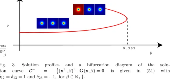
0.333 β v PSfrag replacements R3N β
Fig. 3. Solution profiles and a bifurcation diagram of the solu-tion curve C− = ©(x>, β)>| G(x, β) = 0 is given in (51) with
δ12= δ13= 1 and δ23 = −1, for β ∈ R+}.
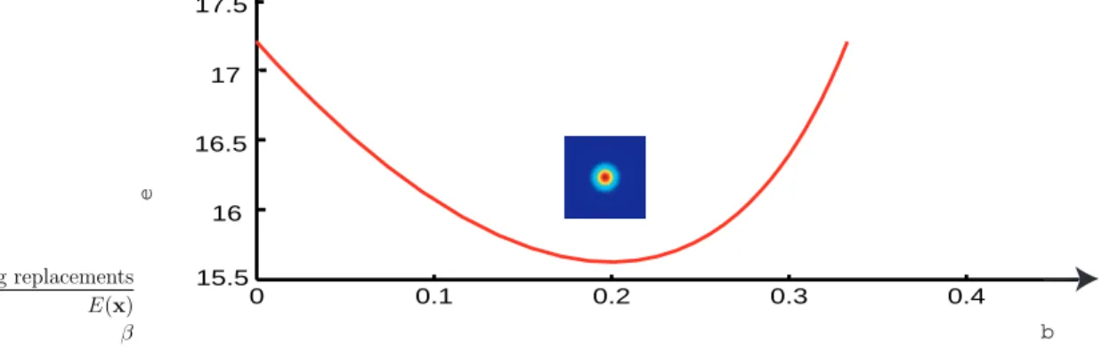
0 0.1 0.2 0.3 0.4 15.5 16 16.5 17 17.5 b e PSfrag replacements E(x) β
Fig. 4. Energy curve of C−.
described in (52b), by computing the set of solution curves
C− =n(x>, β)>| G(x, β) = 0 is given in (51) with (79) δ12 = δ13 = 1 and δ23= −1, for β ∈ R+}
of positive bound state solutions of (51) on a squared domain [−5, 5] × [−5, 5] with grid size h = 0.2. In Figures 3 and 4, we plot the bifurcation diagram of the solution curve and the energy curve, respectively, for β ∈ [0, 0.5]. Similar to the results reported for Simulation 1, nodal domains of positive bound state solutions are attached near the solution curve and the energy curve.
We highlight following observations from Simulations 1 and 2 that are consis-tent with the solution characters shown in Theorem 5.
• In Figure 1 of Simulation 1, the β’s in the primal stalk keeps approaching, but never reach, 1. In contrast, Figure 3 of Simulation 2 shows that a turning point is observed on the primal stalk at β = 0.333, which corresponds to the case of β = −1
3 in Theorem 5.
• As shown in Figure 2, the primal stalk energy curve (plotted in red) keeps rising as β increases. This phenomenon is in line with (62).
• The computed solution profiles of C− not only have the property as shown
in (63), but Figure 3 further shows that the u1 turns to negative side after
passing the turning point.
• As Theorem 6 discusses the number of bifurcation points, we note that it is proved in [20, Lemma 1] that the number of nonnegative eigenvalues of
4φ − φ + 3ω2 ∗φ = λφ, φ ∈ H2(Rn),
is n + 1, where ω∗ is the unique solution of 4φ − φ + φ3 = 0, φ > 0 in Rn, ω(x) → 0 as |x| → ∞.
In the 3-coupled DNLSEs (53) with a squared domain (n = 2), we can verify numerically that the number of nonnegative eigenvalues of Λ1(0) =
σ(A − I + 3[[u°2
∗ ]]) is 3, where u∗ is given in (61).
Simulation 3: If δ12 = δ13= 1, δ23= −1 (the same assumption in Simulation
2) and β is sufficiently small, it can be shown that there exists a non-radially symmetric positive solution and the corresponding energy is smaller than the energy of the positive solution given in (55) [20]. However, only radially sym-metric solutions are found for small β’s in Simulation 2 as shown in Figure 3. To compute the non-radially symmetric positive solution described in [20], we suggest the following procedures.
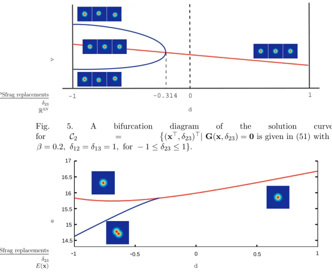
0 1 -1 v d -0.314 PSfrag replacements δ23 R3N
Fig. 5. A bifurcation diagram of the solution curve
for C2 = © (x>, δ 23)>| G(x, δ23) = 0 is given in (51) with β = 0.2, δ12= δ13= 1, for − 1 ≤ δ23≤ 1}. -1 -0.5 0 0.5 1 14.5 15 15.5 16 16.5 17 d e PSfrag replacements δ23 E(x)
0.969 b v PSfrag replacements β R3N
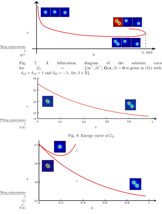
Fig. 7. A bifurcation diagram of the solution curve
for C3 = ©(x>, β)>| G(x, β) = 0 is given in (51) with δ12= δ13= 1 and δ23= −1, for β ∈ R}. 0 0.2 0.4 0.6 0.8 1 11 12 14 16 18 e b PSfrag replacements β E(x)
Fig. 8. Energy curve of C3.
0 0.2 0.4 0.6 0.8 1 11 13 15 17 e b n c PSfrag replacements β C3 C− E(x)
Fig. 9. Comparing with C−, the solution curve C
3 has lower energies.
Step 1. Let
C1 =
n
(x>, β)>| G(x, β) = 0 is given in (51) with (80)
We trace the solution curve in β from 0 to 0.2 by the hyperplane-constrained continuation method.
Step 2. For fixed β = 0.2, we trace the solution curve C2 =
n
(x>, δ23)>| G(x, δ23) = 0 is given in (51) with (81)
β = 0.2, δ12 = δ13 = 1, for − 1 ≤ δ23≤ 1}
in δ23 from +1 to −1 by the hyperplane-constrained continuation method.
Step 3. For fixed δ23 = −1, we trace the solution curve
C3 =
n
(x>, β)>| G(x, β) = 0 is given in (51) with (82) δ12= δ13= 1 and δ23 = −1, for β ∈ R}
in β from 0.2 to 0 and 0.2 to 1 by the hyperplane-constrained continuation method.
We compute the solution curves by following the previous steps on a squared domain [−5, 5] × [−5, 5] with grid size h = 0.2. In Figures 5 and 6 (7 and 8), we plot the bifurcation diagram and the corresponding energy curves of C2 (C3), respectively. Nodal domains of the positive bound state solutions are
attached near the solution curve and the energy curves. The motivation of the above procedure and some observations are highlighted as follows.
(1) The continuation path is followed by increasing β’s from zero to a certain value, which is 0.2 in our experiment specifically. We consider these in-termediate solutions as all ground state solutions corresponding to each of the β’s, as suggested by the following observations. First, since all the interactions are attractive (i.e. δ12, δ13, δ23 > 0), the three components
tend to gather together and concentrate at the center of the domain. Such solution profiles are similar to the ones of the initial solution obtained by letting β = 0. Second, since there is no bifurcation found for 0 ≤ β ≤ 0.2, the states of the solutions are thus unchanged. Furthermore, the solution corresponding to β = 0 is actually the ground state solution according to Section 2, and it is likely that all the computed solutions remain the ground state solutions for 0 ≤ β ≤ 0.2.
(2) The curve C2 acts as a “bridge” connecting the two settings used in Step
1 (three attractive interactions) and 3 (one repulsive and two attractive interactions). Therefore, β is fixed and δ23 is changed from 1 to −1.
Fig-ure 5 shows that there is only one bifurcation point in C2. If we trace the
primal stalk of C2 (the red line), the terminal point attains the primal
stalk of C− in Simulation 2. However, if we trace the bifurcation branch bifurcated at δ23 = −0.231, new solution forms are observed.
Further-more, as shown in Figure 6, the solutions of this bifurcation branch have lower energies compared with the ones on the primal stalk.
interactions are assumed. In this setting, a non-radially symmetric ground state solution exists for β sufficiently small [20]. To obtain this particular solution, we trace C3 by starting from a C2 bifurcation branch solution
that δ12 = 1, δ13 = 1, δ23 = −1 and decreasing β’s from 0.2 to 0. As
shown in Figure 7, non-radially symmetric solutions can be obtained while β’s approach zero. Furthermore, it is worth noting that another type of non-radially symmetric positive solution can be found by increasing β’s from 0.2 to 1. This type of solutions is shown in Figure 7 for β ≈ 0.969. (4) In Figure 9, we compare energy curves of C3 and C−. It shows that the
energy curve of C3 is lower than that of C−. This result is obviously
consistent with the consequence reported in [20]. Besides, the two types of non-radially symmetric positive solutions shown in Figures 7 and 8 are expected to be the ground state solutions of (51), as we start from the ground state solution in C1 for β = 0 and then trace the path with lower
energy solutions in C2 whenever bifurcation occurs.
Acknowledgments
This work is partially supported by the National Science Council and the National Center for Theoretical Sciences in Taiwan.
References
[1] N. Akhmediev and A. Ankiewicz. Partially coherent solitons on a finite background. Phys. Rev. Lett., 82:2661–2664, 1999.
[2] E. L. Allgother and K. Gerog. Numerical path following. In P. G. Ciarlet and J. L. Lions, editors, Handbook of Nemerical Analysis, volume V. Elsevier, 1997. [3] S. L. Chang amd C. S. Chien and B.W. Jeng. Liapunov-schmidt reduction and continuation for nonlinear Schr¨odinger equations. SIAM J. Sci. Comput., 27:729–755, 2007.
[4] W. Z. Bao. Ground states and dynamics of multi-component Bose-Einstein condensates. SIAM Multiscale Modeling and Simulation, 2(2):210–236, 2004. [5] W. Z. Bao and Q. Du. Computing the ground state solution of Bose-Einstein
condensates by a normalized gradient flow. SIAM J. Sci. Comput., 25(5):1674– 1697, 2004.
[6] M. Berry. Large scale singular value computations. Internat. J. Supercomputer
Appl., 6(1):13–49, 1992.
[7] T. F. Chan. Deflation techniques and block-elimination algorithm for solving bordered singular systems. SIAM J. Sci. Stat. Compu., 5:121–134, 1984.
[8] S. M. Chang, Y. C. Kuo, W. W. Lin, and S. F. Shieh. A continuation BSOR-Lanczos-Galerkin method for positive bound states of a multi-component Bose-Einstein condensate. J. Comp. Phys., 210:439–458, 2005.
[9] S. M. Chang, W. W. Lin, and S. F. Shieh. Gauss-Seidel-type methods for energy states of a multi-component Bose-Einstein condensate. J. Comp. Phy., 202:367–390, 2005.
[10] K. W. Chow. Periodic solutions for a system of four coupled nonlinear Schr¨odinger equations. Phys. Lett. A, 285:319–326, 2001.
[11] W. Govaerts. Stable solvers and block elimination for bordered systems. SIAM
J. Matrix Anal. Appl., 12:469–483, 1991.
[12] W. Govaerts and J.D. Pryce. Mixed block elimination for linear systems with wider borders. IMA J. Numer. Anal., 13:161–180, 1993.
[13] Willy J. F. Govaerts. Numerical methods for bifurcations of dynamical equilibria. SIAM, Philadelphia, 2000.
[14] F. T. Hioe. Solitary waves for n coupled nonlinear Schr¨odinger equations. Phys.
Rev. Lett., 82:1152–1155, 1999.
[15] F. T. Hioe and T. S. Salter. Special set and solutions of coupled nonlinear Schr¨odinger equations. J. Phys. A: Math. Gen., 35:8913–8928, 2002.
[16] T. Kanna and M. Lakshmanan. Exact soliton solutions, shape changing collisions, and partially coherent solitons in coupled nonlinear Schr¨odinger equations. Phys. Rev. Lett., 86:5043–5046, 2001.
[17] H. B. Keller. Lectures on Numerical Methods in Bifurcation Problems. Springer-Verlag, Berlin, 1987.
[18] Y. C. Kuo, W. W. Lin, and S. F. Shieh. Bifurcation analysis of a two-component Bose-Einstein condensate. Physica D, 211:311–346, 2005.
[19] M. K. Kwong. Uniqueness of positive solutions of ∆u − u + up = 0 in Rn. Arch. Rational Mech. Anal, 105(3):243–266, 1989.
[20] Tai-Chia Lin and Juncheng Wei. Ground state of n coupled nonlinear Schr¨odinger equations in Rn, n ≤ 3. Commun. Math. Phys., 255:629–653,
2005.
[21] M. Mitchell, Z. Chen, M. Shih, and M. Segev. Self-trapping of partially spatially incoherent light. Phys. Rev. Lett., 77:490–493, 1996.