Abstract—Nonlinearity and time-varying dynamics of fuel cell (FC) systems make it complex to design a controller for improving the output performance. This paper introduces an application of model reference adaptive control to a low power proton exchange membrane (PEM) FC system, which consists of three main components: a FC stack, an air pump to supply air, and a solenoid valve to adjust hydrogen flow. From the system perspective, the dynamic model of PEMFC can be expressed as a multivariable configuration of two inputs, hydrogen and air flow rates, and two outputs, cell voltage and current. The corresponding transfer function can be identified off-line to describe the linearized dynamics with a finite order at a certain operating point, and is written in a discrete-time auto-regression moving-average model for on-line estimation of parameters. This provides a basis of adaptive control strategy to improve the FC performance in terms of efficiency, transient and steady-state specifications. Experiments show that the proposed adaptive controller is robust to the variation of FC system dynamics and power request.
I. INTRODUCTION
ROTON exchange membrane FCs, also known as polymer
electrolyte membrane FCs, have the advantages of high power and energy density, long cell and stack life, low operation temperature, fast start-up, low corrosion, and higher efficiency, compared to most batteries and other FC technologies. FCs are subject to various situations of time-varying load, during which the air flow, gas pressure, temperature, humidity, membrane hydration must be controlled over a wide range of operation. A series of operations require prompt measurements of system states by a set of sensors, such as flowmeter, thermocouples, pressure transducer, voltmeter, hall sensor, hydrogen detector, etc. These signals are fed back to the microprocessor to calculate proper control actions executed by various actuators, such as air pump, humidifier, solenoid valves, fan motors and safety devices.
Manuscript received March 9, 2007. This work was supported in part by National Science Council of Republic of China under Contract NSC 94-2218-E-002-052.
Y. P. Yang is with the Department of Mechanical Engineering, National Taiwan University, No. 1Roosevelt Road, Taipei, Taiwan 10617, Republic of China. (phone: 886-2-3366-2682; fax: 886-2-2363-1755; e-mail: ypyang@ ntu.edu.tw).
Z. W. Liu is now with the Department of Mechanical Engineering, National Taiwan University, No. 1Roosevelt Road, Taipei, Taiwan 10617, Republic of China. (e-mail: [email protected]).
F. C. Wang is with the Department of Mechanical Engineering, National Taiwan University, No. 1Roosevelt Road, Taipei, Taiwan 10617, Republic of China. (phone: 886-2-3366-2680; fax: 886-2-2363-1755; e-mail: fcw@ ntu.edu.tw).
The complex, nonlinear dynamics of FC systems are usually approximately described by the principles of electrochemistry and thermodynamics; and in terms of physical parameters, material properties and universal constants under various assumptions and constraints. The voltage and current variations respond to the faster dynamics of FCs, involving reactant pressure and flow rate, while the slow dynamics of temperature regulation and heat dissipation dominate the steady state response. Many researchers have devoted themselves to the steady-state model of PEMFCs, describing the relationship between physical variables through Nernst equation, gas diffusion equation, concentration, etc. Most recently, an increasing number of researches have focused on dynamic models for describing the transient response of PEMFC systems. Pukrushpan et al. [1] modeled transient dynamics with a set of differential equations governing air compressor, mass transportation, energy conservation of the reactant flows and pressures in the cathode and anode. Ceraolo et al. [2] provided partial differential equations to describe both static and dynamic behaviors of the PEMFC, including gas diffusion, proton concentration, mass transportation, etc. In their spatial, time-dependent FC model, Golbert and Lewin [3] included dynamics of water condensation, evaporation and generation, as well as quasi-steady-state temperature profile. Pathapati et
al. [4] derived a dynamic model with the effects of charge
double-layer capacitance, dynamics of flow and pressure, and mass/heat transient features of FCs, which predicted the transient response of cell voltage, temperature, gas flow rates, pressures under sudden change in load current.
No matter how complex the FC dynamic model is, it never describes system responses precisely in terms of system parameters. The nonlinearity and time-varying characteristics inevitably pose difficult problems on system identification and control. Simplified models, either linear or nonlinear, with nominal parameters are usually valid within a linear range of operation. Such models are usually used to investigate stability, and controllability, before designing a controller. More practically, these parameters are varying with time and operating state, and are identified in real time to match system response with minimal errors. Therefore, adaptive control can serve as a feedback law to achieve control objectives subject to the variation of system parameters as well as external disturbances. Pukrushpan et al. [1] designed an observer- based feedback controller to protect the FC stack from oxygen starvation during changes of current command, using the linear quadratic technique based on the linearized state-space model. Paradkar et al. [5] integrated a linearized PEMFC model into a power plant, and
Model Reference Adaptive Control of a Low Power Proton Exchange
Membrane Fuel Cell
Yee-Pien Yang*, Member, IEEE, Zhao-Wei Liu, and Fu-Cheng Wang
simulated a load frequency control problem by an optimal controller based on the disturbance accommodation control theory. Schumacher et al. [6] employed a fuzzy controller for the humidity management by adjusting the fan voltage for the air supply to a miniature PEM. Jurado and Saenz [7] addressed that their proposed adaptive control strategy was able to stabilize a hybrid FC and turbine system subject to system parameter variations and external disturbances. Meyer and Revankar [8] surveyed the control-oriented models and control strategies of PEMFC systems. They indicated that future attempts to develop nonlinear multi-input multi-output (MIMO) systems, must be important over the entire operating range in order to seek reduced reactant usage under various power demands.
The authors have presented a preliminary study of system identification, robust and adaptive controls of a low power PEMFC [9, 10]. This paper extended the previous single-input single-output (SISO) adaptive control to a multivariable configuration of model reference adaptive control. Both the air and hydrogen flow rates are used to regulate cell voltage and current according to the update information of external load and system dynamics.
II. FCSYSTEM MODEL
In the papers mentioned above, the PEMFC is basically assembled from a series of cells, each of which is composed of an electrolyte sandwiched by anode and cathode electrodes, and each electrode consists of a catalyst and a gas diffusion layer. In order to develop the control strategy of a FC, its dynamic model from previous studies is adopted, describing Nernst equation, cathode gas diffusion, cathode kinetics, and proton concentration dynamics [2, 11-13].
From the system viewpoint, hydrogen is fed at an adjustable flow rate NH, which is regarded as an input
variable. On the other hand, air is often transported by air pump to provide oxygen to the cathode, as well as to the flow rate of air NA, which is also considered an input variable of the
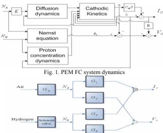
FC. The cell voltage and current are normally chosen as system outputs. From modern control theories [14], the control-oriented FC system block diagram can be approximated as a two-input two-output system as shown in Fig. 1. Equipped with additional balance of plant (BOP), such as air pump and solenoid valve, the FC system can be simply reduced to a standard block diagram in Fig. 2. These coupled blocks, denoted by Gi, i=1, 2, 3, 4, describe the relationships
between outputs, Ic and Vc, and inputs, NA and NH, where R
denotes the internal resistance of FC. Assuming that the FC is operated at a certain operating point, the four blocks can be linearized as transfer functions of finite orders and time-varying coefficients. More specifically, G1 is the transfer
function between Ic and NA, G2 between Vc and NA, G3
between Ic and NH, and G4 between Vc and NH. Therefore, the
FC stack model can be expresses as
VC = G2NA + G4NH - RIC (1)
IC = G1NA + G3NH (2)
This configuration is usually employed as the basis of system identification, as well as an adjustable model for designing the FC controller.
Fig. 1. PEM FC system dynamics
Fig. 2. Approximate FC system block diagram.
III. OFF-LINE SYSTEM IDENTIFICATION
The purpose of off-line system identification is to obtain transfer functions between system inputs and outputs at certain operating points. The information provided from transfer functions, such as system order, parameters, and time delay, must be used for the adaptive controller design. Many approaches are available, but the non-parametric system identification is one of the most effective to investigate the frequency response of FC stack. For a SISO example, the swept sinusoidal input r=γ ωcos texcites the system, and the output y is measured at N-sampled points such that the Dynamic Signal Analyzer (DSA) HP35670A provides the frequency response in terms of magnitude and phase as functions of frequency ω : γ ω) 2 2 2 ( ˆ c s N j I I G = + , (3) c s N N(j ) argGˆ (j ) arctan II ˆ ω = ω =− φ , (4) where 1 ()cos( ) 1 ∑ = = N t c N y t t I ω and 1 ()sin( ) 1 ∑ = = N t s yt t N I ω . The magnitude is usually well fitted by the DSA, but the phase is not due to insufficient information on time delay. Further modification can be achieved by introducing an additional term e ω−j T to the transfer function GˆN(jω) , where T denotes the time delay and is determined by minimizing the cost function
(
)
∑ − = = − n k jT k N k G j e k J 1 2 exp(ω ) arg ˆ ( ω ) ω φ (5)Where φexp(ω is obtained for each sweeping frequency ωk) k
and the resulting transfer function becomes sT N(s)e
Gˆ − .
The system identification is performed on a FC stack of 15 cells, each with an active area of 50 cm2. The cells are
connected with a pre-treated membrane (Nafion® 112) by hot press for optimum conditions, and are electrically connected in series. Platinum coating is about 0.2 mg.cm-2 at anode and
0.4 mg.cm-2 at cathode. The rated and peak power outputs are
117W at 9V and 124W at 7.9V, respectively. The maximum fuel-to-electricity efficiency that the FC can achieve is about 37% on a lower heating value (LHV) under dry H2/air and
humidification-free conditions. The flow rate of air is supplied by an air pump, while the flow rate of hydrogen is regulated by a solenoid valve. Either the cell voltage or current output can be tuned at a specific value with an electronic load meter. Each transfer function Gi is identified
by measuring the corresponding pair of input and output, while fixing the other pair of input and output at their nominal values.
When the cell voltage and hydrogen flow rate are fixed at their nominal values, the transfer function Ga1 between cell
current and air pump voltage, can be identified under certain operating conditions, as depicted in Table 1. It is noticed that the transfer function Ga1 has included the air pump dynamics
Ga implicitly such that Ga1= Ga G1. The flow rate of hydrogen
is fixed, but the output valve opens to purge chemical product for 2 seconds every 2 minutes. The cell voltage is set fixed by a load meter at 8.5, 9, or 9.5V, each with three times. The input voltage of air pump is a sinusoidal function r=
5+2cos(ω ), whose frequency sweeps from 0.05 to 10Hz. t
Then, the DSA takes the measurements of cell current and calculates the magnitude and phase of frequency response according to (3) and (4).
For better fitting to the experimental frequency response, the transfer functions have to be modified by introducing the time delay obtained from (5), and the resulting estimation of transfer function is expressed in different orders as follows:
First order approximation:
s 0703 . 0 1 a (s) 0.01444s s0.2290.08766 e G − + + = (6)
Second order approximation:
s 035 . 0 2 2 1 a e 1392 . 0 s 011 . 1 s 05606 . 0 s 1307 . 0 s 0004543 . 0 ) s ( G − + + + + = (7)
Third order approximation:
s 0475 . 0 2 3 2 3 1 a e 06131 . 0 s 4321 . 0 s 058 . 1 s 02382 . 0 s 06633 . 0 s 1356 . 0 s 002546 . 0 ) s ( G − + + + + + + = (8)
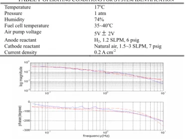
The corresponding frequency responses are shown in Fig. 3. The models do not have significant differences except at high frequencies. A second order transfer function may be sufficient to describe dominant dynamics of a PEMFC stack.
TABLEI OPERATING CONDITIONS FOR SYSTEM IDENTIFICATION
Fig. 3. Identified frequency responses of Ga1 (____experiment, - - - -1st
order, ._._._._.2nd order,···3rd order)
IV. ON-LINE PARAMETER ESTIMATION AND ADAPTIVE
CONTROL
PEMFCs have a number of attributes to make them promising candidates for the use in transportation applications and some domestic appliances. The power demand of automobiles depends on the driving conditions, and the provision of electricity from FC varies from its system states, such as reactant flow rates, cell temperature, humidity, pressure, etc. The relationship between FC output voltage and current is usually described by polarization curves, which also vary with cell temperature, pressure, humidity, and some other states. These time-varying and state-dependent properties are hardly depicted by simple mathematical models, but the system identification proves that it is possible to approximate the FC dynamics by transfer functions at a certain operating point. These transfer functions can be transformed to discrete-time parameter estimation models in the adaptive control loop of FC system subject to external disturbances as well as system parameter changes.
A. ARMA model and on-line parameter estimation
For on-line parameter estimation, the linear system model (1) and (2) is usually represented as a discrete-time equation, and leads to the following the ARMA model [15],
) ( ) , ( ) ( ) , (q k y k B q k u k A = (9) r r 1 1 0(k ) a (k)q a (k )q a ) k , q ( A = + − +" + − (10) r r 2 2 1 1(k)q b (k)q b (k)q b ) k , q ( B = − + − +"+ − (11)
where y denotes the system m-dimensional output vector, u represents the system n-dimensional input vector. The integer
k denotes the time instant of sampling, and r is the system
order. The frequency-dependent delay identified in (6)~(8) has been implicitly placed in the ARMAX model of one-step ahead structure. Without loss of generality, a0=c0=1. In a
succinct form, the term A(q,k)y(k) is the auto-regression part, where q-1 is a backward shift operator and q-hy(k) represents
the past output y(k-h); h=1,2,...r; B(q,k)u(k) denotes the moving average of past inputs, where q-hu(k)=u(k-h).
Therefore, the corresponding transfer function between outputs and inputs in the discrete-time form becomes
) t ( u ) q ( B ) t ( y ) q ( Ai = i . (12) The approach of recursive least square algorithm for system identification is to predict the system output according to the past information of input and output measurements, as well as the update set of system parameters. From (9)-(11), for a0=c0=1, the estimation of y(k) is expressed as
( )k (k 1) (ˆ k 1)
yˆ =φT − θ − (13)
where φT(k-1)=[-y(k-1).. -y(k-m) u(k-1)..u(k-n)] (14)
] cˆ ... cˆ bˆ ... bˆ aˆ ... aˆ [ ˆT = 1 r 1 r 1 r θ (15)
and the estimation error w(k) is defined as y(k)− yˆ(k). At step k, when the new output is measured, the update set of parameters are calculated by [15]
( )k ˆ(k 1) K( ) ( )k
[
yk (k 1) (ˆ k 1)]
ˆ =θ − + −φT − θ − θ (16) ( )k P(k 1) (k 1)[
T(k 1) (P k 1) (k 1)]
1 K = − φ − λ+φ − − φ − − (17) ( )k[
I K ( )k φ (k 1)]
P(k 1)/λ P = − T − − (18) Temperature 17oC Pressure 1 atm Humidity 74% Fuel cell temperature 35~40oCAir pump voltage 5V±2V
Anode reactant H2, 1.2 SLPM, 6 psig
Cathode reactant Natural air, 1.5~3 SLPM, 7 psig Current density 0.2 A cm-2
where the estimation gain K(k) update the parameter estimation, and the covariance matrix P(k) characterizes the difference between the estimated parameters and their true values. Initially, P(0) is chosen a large positive number, for example 103I, where I is an identity matrix, to render the
inaccurate initial guess θˆ(0) quickly negligible. The coefficient 0<λ <1 is called the forgetting factor, which places more importance on the new information for updating system parameters, and less attention on the past information.
B. Model reference adaptive control
Model reference adaptive control is one of the promising strategies for complex FC system. No matter how complicated the system is, its desired output can be designated to follow the output of a reference model with specified dynamics. The model reference adaptive control strategy includes the specification of reference model with desired dynamics, on-line parameter estimation and calculation of control gains. This adaptive control scenario is illustrated in Fig. 4.
Fig. 4. Model reference adaptive control scenario of fuel cell
When FC system is identified and approximated as a second-order model at an instant time t, the plant model is
A(q)y(t)=B(q)u(t) (19)
where A(q)=q2+a
1q+a2, and B(q)=b0q+b1. For a standard
feedback control law
R(q)u(t)=T(q)uc(t)+S(q)y(t), (20)
the closed-loop relationship between uc(t) and y(t) is
) t ( u BS AR BT ) t ( y = + c (21) in which the index q is omitted for simplicity. The desired closed-loop model is chosen as
( ) ( )
m m m c
A y t =B u t , (22) where Am(q)=q2+am1 q+am2 and Bm(q)=bm0 q+bm1, then a
perfect model-following condition becomes
m m
B B T
A R+ B S = A . (23) Under the conditions of compatibility and causality, the polynomials T and S are obtained by the Bezout equation
AR+BS = AmAo, (24) where R(q)=q+r1,S(q)=s0q+s1, and Ao(q)=q+ao is known as an observer polynomial, which is always cancelled in the transfer function from the reference signal to the output. When the unit steady state gain of Bm/Am is designed, and
Bm=β B is selected, the control polynomial T is simply β Ao.
In summary, the parameters of those control polynomials are calculated after system parameters ˆa1, ˆa2, ˆb0, andˆb1are
estimated: 2 1 0 2 0 2 2 1 0 1 2 1 1 1 ˆ (ˆ )ˆ ˆ ˆ ˆ ( ) / m m o m o m r a a b a a a a b b a a a b α ⎡ = ⎣ + − − ⎤ + + − ⎦ (25) 0 1 1 2 1 1 2 1 0 1 2 1 2 2 2 ˆ ( ˆ ˆ ˆ ) ˆ ˆ ˆ ˆ ˆ ( ) / o m m m o m o m o s b a a a a a a a a b a a a a a a a a α ⎡ =⎣ − − + − ⎤ + − − − ⎦ (26) 1 1 1 2 1 2 2 2 2 0 2 2 2 2 1 2 1 ˆ (ˆ ˆ ˆ ˆ ) ˆ ˆ ˆ ˆ ˆ ( ) / m o m o m o m o m s b a a a a a a a a b a a a a a a a a a α ⎡ = ⎣ − + − ⎤ + − − − ⎦ (27) 2 0 2 1 0 1 2 1 ˆ ˆ ˆ ˆ ˆ ˆ a b b a b b − + = α (28) ) ˆ ˆ /( ) (b0m +bm1 b0+b1 = β . (29) V. EXPERIMENTS
From the perspective of certainty equivalence principle in system identification and adaptive control theories, a linear model of reduced order with time-varying parameters is usually used to generate control law as if it were a true system. Three adaptive control scenarios are investigated: the regulation of cell current by air flow rate, the regulation of cell voltage by air flow rate, and the regulation of cell voltage both by air and hydrogen flow rates. The first two are SISO cases, while the last one pertains to the MIMO configuration.
A. Experimental setup
The experimental setup of FC stack and its peripheral devices are schemed in Fig. 5. The on-line parameter estimation and model reference adaptive control law are performed with Matlab on a laptop computer. The FC power is dissipated on an electronic load meter by which either cell current or cell voltage remains constant while the other is regulated. The air flow rate is controlled by an air pump, whose property is specified with the relationship of flow rate and air pressure at various driving voltages, as shown in Fig. 6. The hydrogen flow rate is kept constant of 1.2 standard liter per minute (SLPM) at 6 psig in the SISO cases, but is adaptively controlled by the solenoid valve at on-off sequences. Both the air and hydrogen are not humidified, and the cell temperature is monitored and sequentially controlled around 35~40C.
Fig. 5. Experimental setup of adaptive control of FC
Fig. 6. Air flow rate versus pressure of air pump
Reference Model System Identification and Adjustment Fuel Cell Controller Ru=Tuc-Sy m y c
u
u y θ0 50 100 150 200 250 300 -1 -0.5 0 0.5 Load 8V a1 b1 a2 b0 0 50 100 150 200 250 300 -0.8 -0.6 -0.4 -0.2 0 0.2 0.4 0.6 0.8 1 1.2 Load 4A time(s) a1 b1 a2 b0 0 100 200 300 400 500 600 -2 -1.5 -1 -0.5 0 0.5 1 Load 4A -> 3A -> 2A time(s) a1 b1 a2 b0 0 100 200 300 400 500 600 -1 -0.8 -0.6 -0.4 -0.2 0 0.2 0.4 0.6 0.8 time(s) Load 9V -> 8.5V ->8V a1 b1 a2 b0
B. Regulation of cell current by air flow rate
First, the adaptive control of FC current by the air flow rate is demonstrated. When the output voltage is fixed by the load meter and hydrogen is kept in a steady flow by the solenoid valve, the cell current is adaptively adjusted by the air flow rate or air pump voltage, on the demand of power consumption subject to plant variation. This SISO process is simply described by the transfer function Ga1 which is
transformed into a discrete-time model and easily written in the auto-regression moving-average model with time-varying parameters.
On the current demand of 2A, the load voltage is set at 8V and the hydrogen is supplied continuously with 1.2 SLPM at 7 psig. The time response of air pump voltage input and cell current output are shown in Fig. 7(a), while the corresponding variation of parameters estimated on-line is depicted in Fig. 7(b). It is found that the system parameters did not vary much, and the cell current was regulated within 2±0.02A rms by adjusting the air flow rate. When the cell voltage shifts from 9 through 8.5 to 8V, respectively, at 200 and 400 seconds, the current is regulated at 3A by adaptively adjusting the air pump voltage to change the air flow rate, as shown in Fig. 8(a). The parameter estimation is displayed in Fig. 8(b). Various settings of cell voltage mean different operating points, which result in different parameters in the second order transfer function. At the junctions of voltage change, the cell current experienced abrupt rise, but was immediately adapted to its desired value within ±0.02A rms.
(a)
(b)
Fig. 7. (a) Control of cell current (red) by air pump (green) under the cell voltage at 8V, and (b) the corresponding parameter estimation
(a)
(b)
Fig. 8. (a) Control of cell current (red) at 3A by air pump (green) for the cell voltage at 9, 8.5, and 8V, and (b) the corresponding parameter estimation
C. Regulation of cell voltage by air flow rate
In many applications, the power source has to be kept at a constant voltage, while the current is drawn on the demand of load. For example in Fig. 9, the FC has to supply power at a constant voltage 9V when the current of 4A is delivered. The
FC should be working around a certain operating point, but a slight variation of system parameters make the air pump change the air flow rate to keep the cell voltage constant.
In the situation as the power demand changes in Fig. 10, the voltage is well regulated at 8.5V while the cell current is drawn from 4 through 3 to 2A. The system parameters are varying but soon identified at different operating points, while the control law is adaptively changed to keep the cell voltage at constant.
(a)
(b)
Fig. 9. (a) Control of cell voltage (red) at 9V by air pump (green) under the load demand of 4A, and (b) the corresponding parameter estimation
D. Regulation of cell voltage both by air and hydrogen flow rates
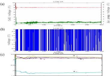
Due to the restriction of the existing component, the hydrogen valve can only be operated in the open and closed states. To make things easier, the air pump still follows the model reference adaptive control law to adjust air flow rate for the cell voltage remaining at constant. But, the hydrogen valve is open when the cell voltage is lower than that is desired, and closed when the cell voltage is higher than desired. The maximum switching frequency of hydrogen valve lies between 3 to 4 Hz, however, the on-off sequences are still oscillatory. The most benefit of the switching control on the hydrogen flow rate is the reduction of the consumption of hydrogen. For example, in Fig. 11(b), the on-off ratio of solenoid valve is about 65:35, meaning the hydrogen consumption is only 65% of that with the valve always on. From Fig. 11(a), the cell voltage is regulated at 8V both by air and hydrogen flow rates, with the stoichiometry of air around 3 and hydrogen around 1.5. During the operation, the parameters of the approximated second-order model Ga2
=GaG2 vary with time as shown in Fig. 11(c), to which,
though, the proposed model reference adaptive controller reveals its robustness.
(a)
(b)
Fig. 10. (a) Control of cell voltage (red) at 8.5V by air pump voltage (green) for the load demand of 4, 3, and 2A, and (b) the corresponding parameter estimation
0 50 100 150 200 250 300 -1.5 -1 -0.5 0 0.5 Load 2A time(s) a1 b1 a2 b0 0 100 200 300 400 500 600 -1 -0.8 -0.6 -0.4 -0.2 0 0.2 0.4 0.6 0.8 1 Load 4A -> 3A -> 2A time(s) b a a b 1 1 0 2 (a) (b) (c)
Fig. 11. (a) Control of cell voltage (red) at 8V both by air pump (green) and (b) solenoid valve switching under the load demand of 2A, and (c) the corresponding parameter estimation
In the situation that the load current demand varies from 4, 3, to 2A at 200 and 400 seconds, as shown in Fig. 12, the voltage is regulated well at 8V by both the air and hydrogen flow rates. The hydrogen flow rate, which is estimated from the on/off ratio in Fig. 12(b), is reduced to 59% with the on-off sequential control of solenoid valve. The multi-input single-output control with model reference adaptive strategy results in the robust performance to the parameter variation shown in Fig. 12(c) in different power demand.
(a)
(b)
(c)
Fig. 12. (a) Control of cell voltage (red) at 8V both by air pump (green) and (b) solenoid valve switching under the load demand from 4, 3, through 2A, and (c) the corresponding parameter estimation
VI. SUMMARY AND CONCLUSION
Model reference adaptive control has been successfully applied to a PEMFC. First, for the control-oriented purpose, the nonlinear, time-varying FC system of electrochemical reactions is approximated by a two-input two-output block system. These blocks describe the dynamic relationship between outputs of cell voltage and current and inputs of hydrogen and air flow rates. Their corresponding transfer function can be identified off-line at certain operating points via a non-parametric frequency domain method, and is reduced to an ARMA model for the on-line parameter estimation in an adaptive control loop. Experimental results
show that the adaptive control is very effective on the regulation of cell current and voltage by the air and hydrogen flow rates, subject to the variation of FC dynamics as well as external power demands. The on-off control of hydrogen valve reduces the fuel consumption. Better scheme on the hydrogen valve control is to be developed, such as fuzzy control, neural network control, etc. It is noteworthy that the successful regulation of cell voltage by air pump and hydrogen valve may relieve DC/DC converters of the effort on regulating the fluctuating cell voltage. Although, this paper has not fully explored the model reference adaptive control in a complete MIMO configuration, nor has been included thermal and water management; the proposed model reference adaptive control should become a promising solution to the FC control both for stationary and transportation power applications.
REFERENCES
[1] J. T. Pukrushpan, A. G. Stefannopoulou, and H. Peng, “Control of fuel cell breathing,” IEEE Control System Magazine, 2004, pp.30-46.
[2] M. Ceraolo, C. Miulli and A. Pozio, “Modelling static and dynamic behavior of proton exchange membrane fuel cells on the basis of electro-chemical description,” Journal of Power Sources, Vol. 113, 2003, pp.131-144.
[3] J. Golbert and D. R. Lewin, “Model-based control of fuel cells: (1) regulatory control,” Journal of Power Sources, Vol. 135, 2004, pp.135-151. [4] P. R. Pathapati, X. Xue and J. Tang, “A new dynamic model for predicting transient phenomena in a PEM fuel cell system,” Renewable Energy, Vol. 30, May 2005, pp. 1-22.
[5] A. Paradkar, A. Davari, A. Feliachi, T. Biswas, “Integration of a fuel cell into the power system using an optimal controller based on disturbance accommodation control theory,” Journal of Power Sources, Vol. 128, 2004, pp. 218-230.
[6] J. O. Schumacher, P. Gemmar, M. Denne, M. Zedda, M. Stueder, “Control of miniature proton exchange membrane fuel cells based on fuzzy logic,” Journal of Power Sources, Vol. 129, 2004, pp.143-151.
[7] F. Jurado and J. R. Saenz, “Adaptive control of a fuel cell-microturbine hybrid power plant,” IEEE Transactions on Energy Conversion, Vol. 18, No. 2, pp.342-347, June 2003.
[8] R. T. Meyer and S. Revankar, “A survey of PEM fuel cell system control models and control developments,” Proceedings of FuelCell06: The Fourth International Conference on Fuel Cell Science, Engineering and Technology, Irvine, California, June 19-21, 2006, Paper No. 97030.
[9] Yee-Pien Yang, Fu-Cheng Wang, Hsin-Ping Chang, Ying-Wei Ma, Chih-Wei Huang, Biing-Jyh Weng, “Low power proton exchange membrane fuel cell system identification and adaptive control,” Journal of Power Sources, Volume 164, Issue 2, 10 February 2007, pp. 761-771.
[10] Fu-Cheng Wang, Yee-Pien Yang, Chi-Wei Huang, Hsin-Ping Chang and Hsuan-Tsung Chen, “System identification and robust control of a portable proton exchange membrane full-cell system,” Journal of Power Sources, Volume 164, Issue 2, 10 February 2007, pp. 704-712.
[11] R. F. Mann, J. C. Amphlett, M. A. I. Hooper, H. M. Jensen, B. A. Peppley and P. R. Roberge, “Development and application of a generalized steady-state electrochemical model for a PEM fuel cell,” Journal of Power Sources, Vol. 86, 2000, pp.173-180.
[12] S. Yerramalla, A. Davari, A. Feliachi, T. Biswas, “Modeling and simulation of the dynamic behavior of a polymer electrolyte membrane fuel cell,” Journal of Power Sources, Vol. 124, 2003, pp.104-113.
[13] J. M. Correa, F. A. Farret, and L. N. Canha, “An analysis of the dynamic performance of proton exchange membrane fuel cells using an electrochemical model,” IECON’01, The 27th Annual Conference of the IEEE
Industrial Electronics Society, 2001, pp.141-146.
[14] G. F. Franklin, J. D. Powell, and A. Emami-Naeini, Feedback Control of Dynamic Systems, 5th edition, Pearson Prentice Hall, 2006.
[15] G. C. Goodwin and K. S. Sin, Adaptive Filtering Prediction and Control, Prentice-Hall, Englewood Cliffs, N.J., 1984.