國
立 交 通 大 學
電機與控制工程學系
博 士 論 文
以 Petri Net 設計之自動化程序遠端監控系統
Design of the Remote Supervision System for
Automated Processes via the Petri Net Approach
研 究 生 : 李 俊 賢
指導教授 : 徐 保 羅 博士
以 Petri Net 設計之自動化程序遠端監控系統
Design of the Remote Supervision System for
Automated Processes via the Petri Net Approach
研 究 生: 李 俊 賢
Student: Jin-Shyan Lee
指導教授: 徐 保 羅 博士
Advisor: Dr. Pau-Lo Hsu
國 立 交 通 大 學
電機與控制工程學系
博 士 論 文
A Dissertation
Submitted to Department of Electrical and Control Engineering College of Electrical Engineering and Computer Science
National Chiao-Tung University In Partial Fulfillment of the Requirements
For the Degree of Doctor of Philosophy
in
Electrical and Control Engineering July 2004
Hsinchu, Taiwan, Republic of China.
以 Petri Net 設計之自動化程序遠端監控系統
研究生:李俊賢
指導教授:徐保羅 博士
國立交通大學
電機與控制工程學系
摘
要
近年來,由於網際網路的快速發展,使得自動化程序之即時監控與管理不再受限於 局部的區域來執行。對於以網際網路為基礎的遠端製造系統,本文闡述其一系列以Petri net 為基礎,在程序控制,遠端監控,與網路管理系統上之設計與實現的方法,以達成 系統之正常安全與運作。 對於日益複雜的製造系統,傳統之階梯圖程序控制設計,不但變的相當複雜,而且 對於製程變動的彈性處理也更加困難。有鑑於此,本文先提出一套以法則為基礎的評估 方法,來驗證Petri net 在程序控制器設計上優於階梯圖的特性。之後,本文提出一套以 Petri net 為基礎,而以階梯圖實現之系統化設計方法,來發展製造系統之程序控制器。 在遠端監控系統中,本文提出一個以監督器 (supervisor) 監控人類行為的架構,來 預防與禁止不正當的遠端人為操作。本文使用Petri net 來塑造命令層中真實系統的抽像 模型,合成出監督器,並進一步使用 Java 技術將監督器實現成一智慧型代理人 (intelligent agent)。藉由遠端受控系統的狀態回饋,我們發展的監控代理人會防止在違反 安全規格下的命令,藉以降低及減少人為失誤所產生的影響。此外,在上述的監控系統 中,為了降低監控器的合成複雜度,我們提出一個階層式的遠端監控架構,使得監督器此外,對於大型遠端監控系統中各種不同的感測、致動、與控制元件,為了管理網
路中各元件所收發的大量監控訊息,本文整合Petri net 於統一建模語言(unified modeling language, UML)中,以系統化地從建模,設計,分析,驗證,來實現簡易網路管理協定 (simple network management protocol, SNMP) 代理人。本研究所提出之遠端網路管理方 法,已經成功地應用在台灣大哥大的行動交換機房之環境安全遠端監控系統上。
Design of the Remote Supervision System for
Automated Processes via the Petri Net Approach
Student: Jin-Shyan Lee
Advisor: Dr. Pau-Lo Hsu
Department of Electrical and Control Engineering
National Chiao-Tung University
ABSTRACT
Applications of the Internet technology become more popular in the modern industry. This thesis proposes the systematic design and implementation of remote supervision systems for automated processes via the Petri nets (PN) approach to achieve 1) the sequence controller, 2) the supervisor, and 3) the device management system, respectively.
As automated systems become more complex, traditional ladder logic diagram (LLD) design of sequence controllers becomes more difficult and inflexible. Thus, this thesis presents a rule-based evaluation to adequately compare the LLD and PN, and verify the superiority of PN. Then, since LLD is still widely used today in real industry, this thesis proposes a PN-based method systematically leading to the final LLD implementation for the sequence controller design.
In remote control systems, to prevent abnormal operations of humans, a remote supervisory scheme is proposed so that undesirable human operations are prohibited. PN is employed to synthesize both the remote supervisor and the local controller, and the Java
to the status feedback through the Internet, the developed supervisory agent provides allowable commands for operators and disables those operations that violate safety specifications. The possibility of human errors can be thus reduced. Moreover, to reduce the complexity of mentioned supervisory system design, this thesis further proposes a hierarchical structure with a smaller state-space size in supervisor synthesis so as to reduce the design complexity.
Furthermore, to integrate diverse network elements and construct a large-scale and distributed systems for remote supervision systems, this thesis integrates the PN into the unified modeling language (UML) to achieve modeling, design, analysis, verification, and implementation of simple network management protocol (SNMP) agents in the present framework. The developed management system has been successfully applied to a mobile switching center of Taiwan Cellular Corporation for the remote supervision and management of its various environmental devices.
ACKNOWLEDGMENT
博士論文的完成,首先要感謝的是指導教授,徐保羅博士在課業與研究上的
指導,以及生活態度上的相授,在此表達我最深誠的敬意與感謝。
謝謝 New Jersey Institute of Technology 的 Meng-Chu Zhou 教授,在我美國
訪問研究一年期間 (7/1/2003-6/30/2004) 的指導與照顧。感謝 NASA 系統工程
師 Peter Graube 在第二章上的建議,盟立自動化蔡宗憲博士在2001年暑期實習期
間的指導與照顧。感謝口試委員:鄭芳田教授 (成功大學製造工程所)、黃漢邦教
授 (台灣大學機械系)、傅立成教授 (台灣大學電機系)、鄭慕德教授 (台灣海洋大
學電機系)、梁高榮教授 (本校工業工程與管理系)、以及本系胡竹生教授等師長
在論文上的指導與建議。
感謝師門的學長、同學與學弟妹們,在生活及研究上的相互幫助及砥礪。工
研院的沈里正、葉賜旭、王安平,中科院的呂龍騰、黃財富、與中正理工的蒙天
德等學長。碩士班88同梯畢業的明潔、裕淵、永生、與建邦等同學。碩士班學弟
妹們:89梯的清穩、志銘、育憲與生虎,90梯的智迪、旭原、明炫、信宏、啟信
與宜霖,91梯的鎮洲、信銘、育修、正義與松德,92梯的豪聲與致成,93梯的政
衍、政宏與伊婷,94梯的景文、尚玲與議寬,以及現役博士班學弟鎮洲與琮政。
此外,謝謝系辦林滿足、李蜀梅、陳英芝小姐,及施德喜先生在事務上的幫忙。
感謝國科會千里馬計劃,在美國訪問研究上的支持,以及教育部在博士班期
間,出席國際會議上的補助。特別謝謝志剛立川夫婦、曉峰、景功、天志、叢哲
夫婦、梅梅夫婦等友人,以及NJIT台灣同學會,在我美國訪問期間生活上的照顧。
謹將此論文獻給我最敬愛的父親 李金柱先生與母親 陳玉雲女士,雅琪姐與
俊德弟,大姑姑 李金枝女士及其家人,以及貼心的女友彥蓉及其家人,因為有
您們的支持與關懷,我才能夠無後顧之憂地,繼續往前邁進。
TABLE OF CONTENTS
Page
ABSTRACT (CHINESE)
i
ABSTRACT (ENGLISH)
iii
ACKNOWLEDGMENT
v
TABLE OF CONTENTS
vi
LIST OF TABLES
ix
LIST OF FIGURES
x
CHAPTER 1
INTRODUCTION
1
1.1. General Review 2 1.2. Problem Statement 5 1.3. Proposed Approach 7 1.4. Organization of Thesis 8CHAPTER 2
EVALUATION OF LADDER LOGIC DIAGRAMS AND
PETRI NETS FOR SEQUENCE CONTROLLER DESIGN
9
2.1. Introduction of Petri Nets 10
2.2. The Rule-Based Comparison 13
2.3. Example: A Stamping Process 18
2.4. Discussions 28
CHAPTER 3
DESIGN OF THE SEQUENCE CONTROLLER IN
MANUFACTURING SYSTEMS
30
3.1. Simplified Petri Net Controller 30
3.2. The IDEF0/SPNC/TPL/LLD Approach 33
3.3. Example: A Stamping Process 41
3.4. Summary 42
CHAPTER 4
REMOTE SUPERVISION FOR
HUMAN-IN-THE-LOOP SYSTEMS
45
4.1. A Novel Supervisory Structure 45
4.2. Design of the Supervisor Using PN 46 4.3. Implementation of the Supervisor Using Java 50
4.4. Example: A Rapid Thermal Process 54
4.5. Summary 62
CHAPTER 5
HIERARCHICAL SUPERVISION FOR
MANUFACTURING SYSTEMS
63
5.1. Proposed Hierarchical Structure 63
5.2. Design of the Hierarchical Supervision System 65 5.3. Example: A Three-Recipe Flexible Manufacturing System 67
CHAPTER 6
SNMP-BASED MANAGEMENT SYSTEM
76
6.1. Integration of UML and PN 76
6.2. Requirements of SNMP Agents 78
6.3. UML-Based Modeling for SNMP Agents 81 6.4. Example: A Mobile Switching Center 85
6.5. PN Modeling and Analysis 89
6.6. Architecture Design and Implementation 93
6.7. Discussions 94 6.8. Summary 96
CHAPTER 7
CONCLUSIONS 97
7.1. Summary of Contributions 97 7.2. Future Research 98REFERENCES 101
VITA 110
PUBLICATION LIST
113
LIST OF TABLES
2.1. Basic elements in LLD and PN. 10
2.2. IF-THEN rules for LLD and PN. 15
2.3. Comparison of LLD and PN for the sequence: A+, A-. 17 2.4. IF-THEN formats of LLD and PN in Fig. 2.4-2.8. 26
3.1. Notations for the stamping process. 44
4.1. Notations for the PN of the RTP system in Fig. 4.6. 58 4.2. Notations for supervisory places of PN in Fig. 4.7. 59
5.1. Notations for the PN of the FMS in Fig. 5.3. 70 5.2. Notations for supervisory places of the PN in Fig. 5.4. 72 5.3. Comparison between the nonhierarchical and hierarchical schemes. 74
LIST OF FIGURES
1.1. Architecture of the proposed remote supervision system in this
thesis. 2
2.1. Basic PN models for (a) sequential, (b) concurrent, (c) cyclic,
(d) conflicting, and (e) mutually exclusive relations. 13 2.2. The LLD and PN for the sequence: A+, A-. 17
2.3. The stamping system. 19
2.4. LLD and PN for Sequence_1. 21
2.5. LLD and PN for Sequence_2. 22
2.6. LLD and PN for Sequence_3. 23
2.7. LLD and PN for Sequence_4. 24
2.8. LLD and PN for Sequence_5. 25
2.9. Required basic elements in the basic element approach. 27 2.10. Required rules and logical operators in the IF-THEN transformation. 27 2.11. The increase ratio for the basic element approach. 28 2.12. The increase ratio for the IF-THEN transformation. 28
3.1. The comparison between the PN and the SPNC via a simple
process. (a) Ordinary PN. (b) SPNC. (c) Comparison results. 31
3.2. The icon definition of the SPNC. 32
3.3. Design procedure of the IDEF0/SPNC/TPL/LLD approach. 34
3.5. The transformation from the IDEF0 to the SPNC. 37 3.6. The transformation from the SPNC to the TPL. 38 3.7. The transformation from the TPL to the LLD. 40 3.8. The transformations of the IDEF0/SPNC/TPL/LLD approach. 40
3.9. The stamping system. 41
3.10. Design of the sequence controller using IDEF0/SPNC/TPL/LLD approach. 43
4.1. (a) Typical remote control system with the human in the loop.
(b) The proposed remote supervisory control scheme. 46 4.2. (a) A general model for door and valve components. (b) The
mutual exclusion specification model. (c) The composed
supervisor for the door-valve system. 50
4.3. Implementation architecture of the remote supervisory control system. 52 4.4. Interactive modeling with sequence diagram for the remote
supervisory control system. 53
4.5. Schematic diagram of the RTP system. 55
4.6. The PN model for automatic control of the RTP system. 57 4.7. The composed PN model for manual control of the RTP system. 57 4.8. Interactive web page for remote control of the RTP system by a
Java applet (only Auto-Control button is admissible in the
automatic control mode). 60
4.9. Interactive web page in manual control mode at Step 3 of RTP
processing (seven buttons are enabled). 61
5.1. Proposed three-level architecture for hierarchical supervision. 64 5.2. Schematic diagram of the three-recipe FMS. 68 5.3. Preliminary PN model of the three-recipe FMS. 69 5.4. Composed PN model of the three-recipe FMS. 71 5.5. PN models of (a) loading, (b) conveying, and (c) processing
tasks for FMS. 72
5.6. Interactive Web page for remote supervision of the FMS by a
Java applet (only three buttons are admissible). 73
6.1. The systematic development procedure for SNMP agents. 79 6.2. The simple network management protocol (an extension of
Stallings, 1993). 80
6.3. Functional analysis with the use-case diagram. 82 6.4. Interaction analysis with the sequence diagrams for (a) the
Request scenario and (b) the Trap scenario. 83 6.5. The SNMP-based remote monitoring and control system. 86 6.6. The class diagram of the SNMP-based monitoring and control system. 88 6.7. The PNs of the SNMP-based monitoring and control system. 91 6.8. Architectural design with the deployment diagram. 95 6.9. The hardware setup during prototype development. 96
Chapter 1
Introduction
Recently, with the rapid development of information technology on industrial applications, remote monitoring, control, and management are critical to increase safety and flexibility of modern manufacturing processes in real operations. Some issues in e-automation are extensively discussed like: the integration of the high level message management and the fundamental layer sequence control, the effect of human errors in remote control, and the efficient message management among various devices on the networks, etc.
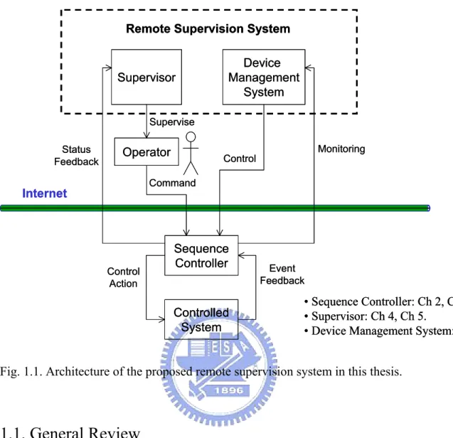
Generally, an automated system implements a sequence controller to regulate local processes. Also, a supervisor is required to assure normal operations, and a device management system is required to administer the various elements efficiently and flexibly. In this thesis, a remote supervision system will be developed for automated processes, as shown in Fig 1.1. The design goals of the present remote supervision system are as follows:
1) to develop the sequence controller to regulate the processes. 2) to develop the supervisor to monitor the human behaviors.
3) to develop the device management system to integrate diverse elements on networks.
The developed approaches in this thesis have been studied on a stamping process, a rapid thermal process in semiconductor manufacturing, a three-recipe flexible manufacturing system, and an environmental monitoring system in mobile switching centers, respectively.
Supervisor Event Feedback Control Action Internet Sequence Controller Device Management System Status Feedback Command Control Controlled System Operator Supervise Monitoring Remote Supervision System
• Sequence Controller: Ch 2, Ch 3. • Supervisor: Ch 4, Ch 5.
• Device Management System: Ch 6. Supervisor Event Feedback Control Action Internet Sequence Controller Device Management System Status Feedback Command Control Controlled System Operator Supervise Monitoring Remote Supervision System
• Sequence Controller: Ch 2, Ch 3. • Supervisor: Ch 4, Ch 5.
• Device Management System: Ch 6.
Fig. 1.1. Architecture of the proposed remote supervision system in this thesis.
1.1. General Review
Basically, an automated process is inherently a discrete event system (DES). The Petri net (PN) has been developed as a powerful tool for modeling, analysis, simulation, and control of DES. PN was named after Carl A. Petri (1962), who created a net-like mathematical tool for describing relations between the conditions and the events. PN was further developed to meet the need in specifying process synchronization, asynchronous events, concurrent operations, and conflicts or resource sharing for a variety of industrial automated systems at the discrete-event level. Starting in the late of 1970’s, researchers investigated possible industrial applications of PN in discrete-event systems and results can be found in the survey/tutorial papers of Murata (1989), Zurawski and Zhou (1994), David and Alla (1994), and Zhou and Jeng (1998).
1.1.1 Systematic design of sequence controllers
A sequence controller that deals with the discrete events plays an important role in automated manufacturing systems (Tilbury and Khargonekar, 2001; Frey and Litz, 2000). Basically, the ladder logic diagram (LLD) of the industrial standard IEC1131-3 (International Electrotechnical Commission, 1993) has been widely used in real applications to conduct the control sequences and usually implemented with a programmable logic controller (PLC). The PLC has the advantages of reliability, robustness, and direct programming. The I/O procedures of the PLC are specified by the LLD and automated machines thus perform repetitive operations in sequence. For some simple controlled systems, it is easy to program the LLD with heuristic approaches. However, as systems become more complex, the controller design and the LLD implementation become even more difficult. In addition, because the LLD is usually programmed only to control the process, corresponding qualitative analysis and performance characteristics of the PLC controlled processes are seldom discussed in practice. Since product specifications are varied frequently, LLD programs of machining processes need to be modified and maintained usually with significant efforts. Hence, researchers are pursuing a systematic and efficient approach for the design and implementation of the sequence controller. Based on the PN, Liang and Hong (1994) proposed a hierarchy transformation method to design and implement controllers on a G2 expert system. Uzam and Jones (1998) introduced an extended PN method to analyze a target system and then implemented it via LLD. Feldmann, et al. (1999a, 1999b) used the colored PN to form the structured text (ST) for PLC implementation. In the past few years, the PN approach still attracted more attentions as a potential tool for designing sequence controllers.
1.1.2 Development of supervisory systems
Recently, due to the rapid development of Internet technology, system monitoring and control no longer needs to be conducted within a local area. Several remote approaches have been proposed which allow people to monitor the automated processes from great distances (Weaver et al., 1999; Yang et al., 2002; Kress et al.,
2001; Huang and Mak, 2001; Batur et al., 2000). Practically, to perform maintenance functions in hazardous environments without their exposure to dangers is a unique application of the remote technology. By conducting remote access using IP-based networks, an entire Internet-based control system is inherently a DES and its state change is driven by occurrences of individual events. The supervisory control theory provides a suitable framework for analyzing DES (Ramadge and Wonham, 1987, 1989; Balemi et al., 1993) and most existing methods are based on automata models. The calculus of communicating systems (CCS), which was invented by Robin Milner (1989), is another classical formalism for representing systems of concurrent processes. However, these available methods often involve exhaustive searches of overall system behavior and result in state-space explosion design as system becomes more complex. On the other hand, PN is an efficient approach to model the DES and its models are normally more compact than the automata models. Also, PN is better suitable for modeling systems with parallel and concurrent activities. In addition, PN has an appealing graphical representation with a powerful algebraic formulation for supervisory control design (Giua and DiCesare, 1991; Moody and Antsaklis, 1998; Uzam et al., 2000).
1.1.3 Management of diverse elements on networks
For large-scale and long-distance distributed systems, a reliable management system for all devices and components on the network is crucial to guarantee normal operations. It allows for reliably monitoring the status of processes, correctly detecting abnormal conditions, efficiently activating emergency mechanisms, and proactively reporting alarms. In general, the components of remote management systems can be classified into 1) the agent side and 2) the manager side. Some vendors build their web server software into their agent-side devices and the manager-side users may thus directly monitor them using web browsers through the hypertext transfer protocol (HTTP). However, as numerous devices are networked in automated manufacturing systems, the massive monitoring and control messages from all devices becomes increasingly difficult to handle. In general, straightforward integration with all Web access points is apparently not efficient. One approach to
manage diverse network elements is to use the simple network management protocol (SNMP). It is a standard protocol now widely supported by most device vendors for their products such as routers, bridges, and printers (Stallings, 1993). Aicklen and Main (1995) used SNMP to manage a variety of network elements. Cardoso and Monteiro (1998) applied the SNMP to monitor and control the industrial network. Kunes and Sauter (2001) provided a modular and extendible gateway to connect the high-level Internet and low-level fieldbus for SNMP network management.
1.2. Problem Statement
Although a lot of efforts in the past two decades have been put on the development of sequence controllers, supervision systems, and management systems for automated manufacturing processes with Internet technology, some critical issues still exist in the remote supervision system as discussed in the following:
1. Requirement of adequate evaluation for sequence controller design
Although PN has been studied to design sequence controllers with a potential in its flexibility, it is still argued that whether the PN approach is superior to the traditional LLD design for industrial practitioners. Hence, an adequate comparison is required. In the past, the “basic element” approach was developed to compare the complexity and flexibility between LLD and PN designs (Venkatesh et al., 1994a; Zhou and Twiss, 1998). However, the basic elements of these two designs are inherently different and hence, it may lead to unreliable comparison results. 2. Requirement of systematic sequence controller implementation
In practice, PLC engineers still widely prefer to use LLD for real implementation. However, it is not straightforward to construct the LLD models from a given sequence. Some researchers have attempted to transform PN into LLD (Peng and Zhou, 2001). However, those resultant LLD are usually more complex as compared to that programmed directly by engineers. A systematic approach from a given specification to achieve the final LLD implementation is
thus required.
3. Requirement of supervisory systems for human error prevention
Typically, an Internet-based control system is a “human-in-the-loop” system. The human operator is involved in the loop and use a general web browser or specific software to monitor and control remotely located systems according to the observed status, usually displayed by the state and/or image feedback. However, human operators may send incorrect or improper commands during the operation and research results indicate that approximately 80% of industrial accidents are attributed to human errors, such as omitting a step, falling asleep and improper control of the system (Rasmussen et al., 1994). Therefore, solutions to reduce or eliminate the possibility of human errors are required in Internet-based control systems.
4. Requirement of reducing the complexity of supervisor synthesis
PN can represent the remote control system with a more compact model. However, during the synthesis of the supervisor, the complexity exponentially increases in the state-space size of the subsystems and specifications. This computational expense often makes the supervisor synthesis infeasible, especially for large-scale manufacturing systems.
5. Requirement of management for different networked devices
To design a remote monitoring and control structure through the network, efficient management to handle the massive information flow and represent data from different devices in a uniform format is required. Although using SNMP is a feasible approach to manage diverse network elements, in present industrial applications, many basic components such as sensors, actuators, and PLCs do not support SNMP for remote applications yet. Thus, for those without SNMP functions, a systematic approach to model and implementation SNMP function is required.
1.3. The Proposed Approach
To deal with the above problems, corresponding approaches are proposed in this thesis as follows.
1. Improved evaluation of LLD and PN
A rule-based approach for the LLD and PN evaluation via the IF-THEN transformation is proposed in this thesis. By converting both the LLD and PN into the same IF-THEN format, a unified comparison is then conducted with the same measure, which is the sum of 1) the number of IF-THEN rules, and 2) the number of logical operators, for both LLD and PN.
2. Systematic design of sequence controllers
A systematic approach to the LLD implementation of the sequence controller in manufacturing systems is introduced in this thesis. By defining the sensor state into the PN to form a simplified Petri net controller (SPNC), a more compact LLD structure through the token passing logic (TPL) is obtained. Typically, the sensor state is used to trigger sequences in manufacturing. The integration definition language 0 (IDEF0) can be used to obtain the SPNC model through the material flow diagrams and information flow diagrams in sequence. Thus, the proposed IDEF0/SPNC/TPL/LLD approach, including the IDEF0, SPNC, and TPL tools, leads to the LLD for general PLC implementation.
3. Supervisory control of human behaviors
In this thesis, a supervisory scheme is proposed for the remotely controlled, human-in-the-loop system. The role of a supervisory agent is to interact with the human operator and the controlled system so that the closed human-in-the-loop system meets the required specifications. In the supervision system, the supervisory agent acquires the system status and makes the decision to enable/disable associated events to meet the required safety specifications. The human operator is then only allowed to perform the enabled events to control the system, and hence, the supervisory agent guarantees that undesirable manually executions never occur.
4. Hierarchical supervision of processes
In the present design of supervisory systems, PN can be used to design both the supervisor at the upper level and the local controller at the lower level. This thesis proposes a hierarchical supervision system resulting in a smaller state-space size through the supervisory synthesis. The proposed design guarantees that remote commands meet resource constraints and deadlock-free specifications. Also, fewer request/response transmissions are required for Internet communication. As a result, the effects of time delays and packet losses could be moderated.
5. Modeling and implementation of SNMP agents
A new approach to the development of SNMP agents for managing diverse network elements in manufacturing processes is proposed. The unified modeling language (UML) is adopted for modeling the system, and then the PN model is applied to analyze the dynamic behaviors of the system. In real applications, the present design is implemented with Java and ladder diagrams on the industrial PLC.
1.4. Organization of Thesis
This thesis is organized as that: the improved evaluation of LLD and PN is presented in Chapter 2. Then, Chapter 3 introduces the IDEF0/SPNC/TPL/LLD approach for the sequence controller design. The basic supervisory control scheme for the remote-controlled processes is proposed in Chapter 4, and Chapter 5 extends it to a hierarchical scheme. For device management, Chapter 6 proposes an integrated approach including UML modeling and PN analysis to develop the SNMP agents. Finally, conclusions and recommendations for further research are provided in Chapter 7.
Chapter 2
Evaluation of Ladder Logic Diagrams and Petri Nets
for Sequence Controller Design
Sequence controller designs play a key role in advanced manufacturing systems. Traditionally, the ladder logic diagram (LLD) has been widely applied to programmable logic controllers (PLC), while recently the Petri net (PN) has emerged as an alternative tool for the sequence control of complex systems. The evaluation of both approaches has become crucial and has thus attracted attention.
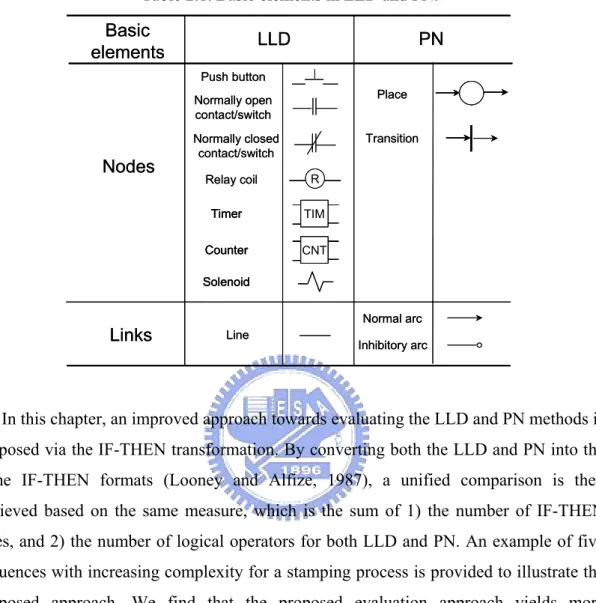
Practically, only a limited amount of research comparing these approaches has been reported, because suitable comparison criteria are difficult to identify. Boucher et al. (1990) studied the sequence control of a manufacturing system and reported that using PN makes the controller more tractable than using LLD. However, they have not formally quantified the comparison between LLD and PN to design sequence controllers. Venkatesh et al. (1994a, 1994b) proposed the number of “basic elements”, which are nodes and links in the LLD and PN, as a quantified measure to compare their design complexity and response time. They claimed that PN offers a better solution than LLD, especially in adaptability as specifications change. Based on the basic element approach, Zhou and Twiss (1995, 1998) further compared the LLD and PN in terms of the understandability, flexibility and the ability to perform correctness verification. They also reported that the PN displays better results. However, note that while basic elements in the LLD stand for push buttons, limited switches, relay coils, timers, counters, solenoids and lines, they are places, transitions and arcs in the PN. Since both nodes and links in the LLD and PN have different physical meaning, as shown in Table 2.1, analysis of LLDs and PNs simply by using the number of basic elements as the comparison measure may lead to an incoherent comparison.
Table 2.1. Basic elements in LLD and PN. Nodes PN LLD Basic elements Place Transition Push button Normally open contact/switch Timer TIM CNT Counter Solenoid Normally closed contact/switch
Links Line Normal arc
R Relay coil Inhibitory arc Nodes PN LLD Basic elements Place Transition Push button Normally open contact/switch Timer TIM CNT Counter Solenoid
Timer TIMTIM CNT CNT CNT Counter Solenoid Normally closed contact/switch
Links Line Normal arc
R R Relay coil
Inhibitory arc
In this chapter, an improved approach towards evaluating the LLD and PN methods is proposed via the IF-THEN transformation. By converting both the LLD and PN into the same IF-THEN formats (Looney and Alfize, 1987), a unified comparison is then achieved based on the same measure, which is the sum of 1) the number of IF-THEN rules, and 2) the number of logical operators for both LLD and PN. An example of five sequences with increasing complexity for a stamping process is provided to illustrate the proposed approach. We find that the proposed evaluation approach yields more reasonable results. Also, the realistic comparisons provided in this chapter support the superiority of the PN approach.
2.1. Introduction of Petri Nets
A PN is identified as a particular kind of bipartite directed graph populated by three types of objects. They are places, transitions, and directed arcs connecting places and transitions. Formally, a PN can be defined as
) , , , (P T I O G= , (2.1) where,
P = {p1, p2,…, pm} is a finite set of places, where m>0;
T = {t1, t2, …, tn} is a finite set of transitions with P∪T ≠∅ and P∩T =∅,
where n>0;
N T P
I: × → is an input function that defines a set of directed arcs from P to T, where N = {0, 1, 2, …};
N P T
O: × → is an output function that defines a set of directed arcs from T to P. A marked PN is denoted as (G, M0), where M0 : P → N is the initial marking. A
transition t is enabled if each input place p of t contains at least the number of tokens equal to the weight of the directed arc connecting p to t. When an enabled transition fires, it removes the tokens from its input places and deposits them on its output places. PN models are suitable to represent the systems that exhibit concurrency, conflict, and synchronization.
Some important PN properties in manufacturing systems include boundedness (no capacity overflow), liveness (freedom from deadlock), conservativeness (conservation of non-consumable resources), and reversibility (cyclic behavior). The concept of liveness is closely related to the complete absence of deadlocks. A PN is said to be live if, no matter what marking has been reached from the initial marking, it is possible to ultimately fire any transition of the net by progressing through some further firing sequences. This means that a live PN guarantees deadlock-free operation, no matter what firing sequence is chosen. Validation methods of these properties include reachability analysis, invariant analysis, reduction method, siphons/traps-based approach, and simulation (Zhou and Jeng, 1998).
2.1.1 Elementary PN Models
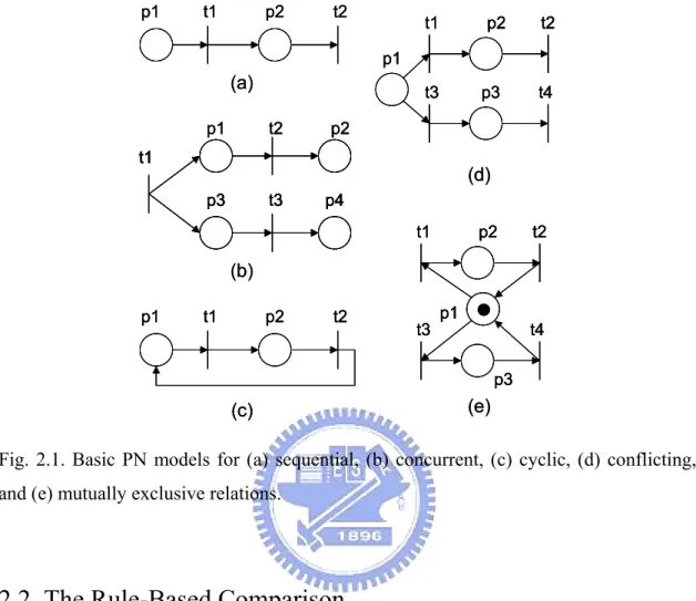
At the modeling stage, one needs to focus on the major operations and their sequential or precedent, concurrent, or conflicting relationships. The basic relations among these processes or operations can be classified as follows.
1) Sequential: As shown in Fig. 2.1 (a), if one operation follows the other, then the places and transitions representing them should form a cascade or sequential relation in PNs. 2) Concurrent: If two or more operations are initiated by an event, they form a parallel structure starting with a transition, i.e., two or more places are the outputs of a same transition. An example is shown in Fig. 2.1 (b). The pipeline concurrent operations can be represented with a sequentially-connected series of places/transitions in which multiple places can be marked simultaneously or multiple transitions are enabled at certain markings.
3) Cyclic: As shown in Fig. 2.1 (c), if a sequence of operations follow one after another and the completion of the last one initiates the first one, then a cyclic structure is formed among these operations.
4) Conflicting: As shown in Fig. 2.1 (d), if either of two or more operations can follow an operation, then two or more transitions form the outputs from the same place.
5) Mutually Exclusive: As shown in Fig. 2.1 (e), two processes are mutually exclusive if they cannot be performed at the same time due to constraints on the usage of shared resources. A structure to realize this is through a common place marked with one token plus multiple output and input arcs to activate these processes.
p2 t1 p1 t2 (a) p1 t2 p2 t1 t3 p3 p4 (b) t2 p1 t3 t1 p2 t4 p3 (d) p2 t1 p1 t2 (c) t2 t3 t1 p2 t4 p3 p1 (e) p2 t1 p1 t1 p2 t2 p1 t2 (a) p1 t2 p2 t1 t3 p3 p4 p1 t2 p2 t1 t3 p3 p4 t1 t3 p3 p4 (b) t2 p1 t3 t1 p2 t4 p3 t2 p1 t3 t1 p2 t4 p3 (d) p2 t1 p1 t1 p2 t2 p1 t2 (c) t2 t3 t1 p2 t4 p3 p1 t2 t3 t1 p2 t4 p3 p1 (e)
Fig. 2.1. Basic PN models for (a) sequential, (b) concurrent, (c) cyclic, (d) conflicting, and (e) mutually exclusive relations.
2.2. The Rule-Based Comparison
Two of major factors for comparison of LLD and PN for sequence control are identified as design complexity and response time (Venkatesh et al., 1994a). Design complexity is defined as the complexity associated in designing the control logic for a given specification. Response time is termed as the scan time in LLD or the execution time in PN. The major factor for design complexity is the physical size of the control logic model, whereas the response time is influenced by not only the physical size, but also the hardware of implementation. For simplicity, this chapter focuses on the comparison of the control logic models. The proposed approach includes two steps as follows:
operators.
In general, control models use smaller number of IF-THEN rules and logical operators are easier to understand, debug, check and maintain. Moreover, they may have a shorter response time. Thus, the proposed approach based on the unified rule-based format to compare the corresponding design complexity and response time for different LLD and PN structures.
2.2.1 IF-THEN Formats
Basically, compound IF-THEN rules, which involve both the conjunctive and disjunctive connectives in their antecedent or conclusion part, can be categorized into the following basic four types (Looney and Alfize, 1987).
Type 1: IF (A and B) THEN C, or expressed as (A∩B) →C, Type 2: IF A THEN (C and D), or expressed as A →(C∩D), Type 3: IF (A or B) THEN C, or expressed as (A∪B) →C, Type 4: IF A THEN (C or D), or expressed as. A →(C∪D).
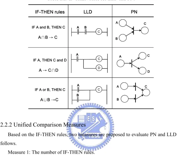
The Type 2 rule can be broken into two simple rules A→C and A→D. Similarly, the Type 3 rule is equivalent to the two simple rules A→C and B→C because the truth of either A or B (or both) implies the truth of C. In practice, since the Type 4 rule does not achieve the specific implication and often causes conflict problems, it is generally not suitable for real applications in the sequence control. The IF-THEN rules excluding Type 4 for the LLD and PN transformations are shown in Table 2.2. Note that the timers and counters can also be expressed in the basic rules. For example, the condition A may represent delaying the desired time units, and the status C may express that a counter increases or decreases one unit.
Table 2.2. IF-THEN rules for LLD and PN. IF A and B, THEN C A∩B → C IF A, THEN C and D A → C∩D IF A or B, THEN C A∪B →C A B C C D A A B C PN D C A B A C C B A LLD IF-THEN rules IF A and B, THEN C A∩B → C IF A, THEN C and D A → C∩D IF A or B, THEN C A∪B →C A B C A B C C D A C D A A B C A B C PN D C A B A C C B A LLD D C A D C A A B A C B B A A C C C B A C B B A A LLD IF-THEN rules
2.2.2 Unified Comparison Measures
Based on the IF-THEN rules, two measures are proposed to evaluate PN and LLD as follows.
Measure 1: The number of IF-THEN rules.
Measure 2: The number of logical operators, including the conjunction (AND), disjunction (OR), block and implication.
The summation of Measure 1 and Measure 2 can be recognized as a new measure for evaluating different structures. By transforming both the LLD and PN to the same IF-THEN formats, comparisons with a unified measure can then be made. Basically, models use smaller number of IF-THEN rules and logical operators are easier to understand, debug, check and maintain. Moreover, they often have a shorter response time. Therefore, the sum of Measure 1 and Measure 2 properly signifies the design complexity and response time for the process represented in either LLD or PN structures.
2.2.3 A Preliminary Comparison
A simple example we use to illustrate the proposed approach is shown in Fig. 2.2, which a piston performs a forward stroke and then retracts. In this figure, the specification A+ indicates a forward stroke and A- indicates return stroke sequentially. Both the LLD and PN controllers as shown in Fig. 2.2 can be either represented by the basic elements or transformed into the same IF-THEN format, as listed in Table 2.3. Results show that the number of basic elements for the LLD and PN are 34 and 22, respectively. However, the basic elements in LLD and PN are physically different, as mentioned before, and the comparison based simply on the number of basic elements for different structures is apparently inappropriate. On the other hand, the results obtained from the IF-THEN transformation indicate that the LLD programming needs 4 IF-THEN rules and 14 logical operators, while the PN only needs 5 IF-THEN rules and 6 logic operators. Therefore, the number of IF-THEN rules and logical operators for LLD and PN is 18 and 11, respectively. Although the results of both approaches indicate that the PN offers a better solution than LLD, the present IF-THEN transformation provides more reasonable results when evaluating different structures in sequence controller design. Furthermore, the degree of programming flexibility can be analyzed by observing the increase ratio of either the number of basic elements or the number of present rules/operators as sequences become more complex.
1. Pb → R1, 2. R1∩a0 → A+, 3. A+ → a1, 4. a1 → A-, 5. A- → a0. 1. ((Pb∩a0)∪R1)∩R2’ → R1, 2. R1 → A+, 3. ((R1∩a1)∪R2)∩a0’ → R2, 4. R2 → A-. R1 Pb a0 R1 R2 a1 R2 R2 a0 R1 A+ R2 A-R1 | a1 | a0 A+ A-Cylinder_A Specification : A+,
A-PN
LLD
IF-THEN formats
Pb Push Pb A+ End {A+} a1 A-Do {A+} a0 R1 Do {A-} End {A-}Comparison
1. Pb → R1, 2. R1∩a0 → A+, 3. A+ → a1, 4. a1 → A-, 5. A- → a0. 1. ((Pb∩a0)∪R1)∩R2’ → R1, 2. R1 → A+, 3. ((R1∩a1)∪R2)∩a0’ → R2, 4. R2 → A-. R1 Pb a0 R1 R2 a1 R2 R2 a0 R1 A+ R2 A-R1 | a1 | a0 A+ A-Cylinder_A Specification : A+,A-PN
LLD
IF-THEN formats
Pb Push Pb A+ End {A+} a1 A-Do {A+} a0 R1 Do {A-} End {A-}Comparison
Fig. 2.2. The LLD and PN for the sequence: A+, A-.
Table 2.3. Comparison of LLD and PN for the sequence: A+, A-.
Comparison measures LLD PN Push button 1 NO contact 7 NC contact 2 Relay 2 Solenoid 2 Line 20 Place 6 Transition 5 Normal Arc 11 Basic elements Total 34 Total 22 Rule 4 Operator 14 Rule 5 Operator 6 IF-THEN rules Total 18 Total 11 Comparison measures LLD PN Comparison measures LLD PN Push button 1 NO contact 7 NC contact 2 Relay 2 Solenoid 2 Line 20 Place 6 Transition 5 Normal Arc 11 Basic elements Total 34 Total 22 Rule 4 Operator 14 Rule 5 Operator 6 IF-THEN rules Total 18 Total 11
2.3. Example: A Stamping Process
To illustrate the proposed approach, we use an industrial process for automatic mark stamping and examine how the specifications change as we consider five increasingly complex sequences.
2.3.1 System Description
As shown in Fig. 2.3, a mark stamping system consists of three cylinders which are operated by four-port and two-way solenoid valves. Each cylinder has two normally open limit switches. For example, when the end of pusher_A contacts the limit switch a0, then a0 is closed, meaning that pusher_A is at the end of its return stoke. The whole system includes 7 input sensors corresponding to 6 limit switches and one push button for starting the system, and 6 output actuators corresponding to 6 solenoid valves. In the stamping process, pusher_A moves the workpiece from a store onto the worktable. Then, the workpiece is stamped by stamper_B and afterwards is ejected by thrower_C. The logical sequence of the stamping system is A+, B+, {A-, B-}, C+, and C-, where {A-, B-} represents two concurrent actions as the pistons of both pusher_A and stamper_B perform return stokes simultaneously. Five sequences with increasing complexity are considered here as follows:
Sequence_1: START, A+, B+, {A-, B-}, C+, C-
Sequence_2: START, A+, B+, 10 sec, {A-, B-}, C+, C- (Sequence_1 with one 10-sec timer added) Sequence_3: START, 3 [A+, B+, 10 sec, {A-, B-}, C+, C-]
(Sequence_2 with one 3-time counter added)
Sequence_4: START, 3 [A+, B+, 10 sec, {A-, B-}, C+, C-], 30 sec, 2 [A+, B+, 10 sec, {A-, B-}, C+, C-]
Sequence_5: Sequence_4 with one emergency stop added.
The complexity of these five sequences increases as specified above.
Stamper_B Thrower_C Pusher_A | a1 | a0 A+ A-Pusher_A | c0 | c1 C+ C-Thrower_C | b0 | b1 B+ B-Stamper_B Stamper_B Thrower_C Pusher_A Stamper_B Thrower_C Pusher_A | a1 | a0 A+ A-Pusher_A | c0 | c1 C+ C-Thrower_C | b0 | b1 B+ B-Stamper_B | a1 | a0 A+ A-Pusher_A | a0 A+ A-Pusher_A | c0 | c1 C+ C-Thrower_C | b0 | b1 B+ B-Stamper_B
Fig. 2.3. The stamping system.
2.3.2 Sequence Controller Design
In order to solve the interlock problem, the LLD programs are usually developed with the assistance of the cascaded method which divides the required sequence into groups (Pessen, 1989). Possible contradictory solenoid signals can be thus avoided. On the other hand, since PN is a concurrent operation, it can be verified to avoid the interlock logic problem via the simulation (Zhou and Venkatesh, 1998). The LLD and PN for the Sequence_1-Sequence_5 are shown in Fig. 2.4-2.8. Although the sequences compared here only consider a typical cylinder-actuating system, similar analysis can be extended to general industrial applications such as motors, pumps, heaters and conveyors.
2.3.3 Comparison of LLD and PN
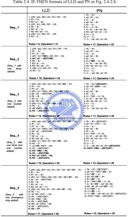
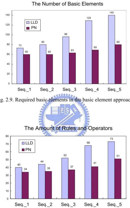
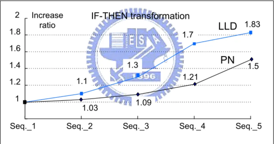
Table 2.4 shows the IF-THEN formats of the LLD and PN in Fig. 2.4-2.8. The required basic elements in the basic element approach, and the required rules and logical operators in the IF-THEN transformation for the five sequences are shown in Fig. 2.9-2.10, separately. For these five sequences, the increase ratio, which is the normalized measure based on Sequence_1 corresponding to the increasing sequence complexity, is also shown in Fig. 2.11-2.12 for the two approaches. In general, a larger ratio indicates that the design is less flexible when subjected to changes in sequence control. All results indicate that the PN is superior to LLD in terms of design simplicity, response time and flexibility responding to the specification changes.
R1 R1 R2 Pb a0 R3c0 R1 a1 A+ B+ R2 R3 b1 R1 R2 R2 a1 b0 a0 B- A-C+ R3 R3 R1 R2c1 R3 C-LLD (a) (b) Sequence_1:
START, A+, B+, {A-, B-}, C+,
C-PN Pb Push Pb A+ End {A+} a1 B+ b1 Do {A+} A- B-R2 b0 a0 Do {C+} C+ End {C+} End {C-} Do {C-} c1 c0 R1 Do {B+} End {B+} Do {A-,B-} End {A-,B-}
Basic element: Nodes = 30, Links = 43 Basic element: Nodes = 26, Links = 34
LLD PN Sequence_2:
START, A+, B+, 10 sec, {A-, B-}, C+, C-(Sequence_1 with one 10-sec timer added)
R1 R1 R2 Pb a0 R3 c0 R1 a1 A+ B+ R2 R3 b1 R1 b0 c0 10 secTIM1 R2 R2 a1 b0 a0 B- A-C+ R3 R3 R1 R2 c1 R3 C-Pb Push Pb A+ End {A+} a1 B+ b1 Do {A+} A- B-R2 b0 a0 Do {C+} C+ End {C+} End {C-} Do {C-} c1 c0 R1 Do {B+} End {B+} End {A-,B-} TIM1, 10sec Do {A-,B-} (a) (b)
Basic element: Nodes = 33, Links = 47 Basic element: Nodes = 26, Links = 34
R1 R1 R2R4 Pb a0 R3c0 R1 a1 A+ B+ R2 R3R4 b1 R1 b0 c0 10 secTIM1 R2 R2 a1 b0 a0 B- A-C+ R3 R3 R1R4 R2c1 R4 c0 Pb 3 timesCNT1 R3 C-LLD Sequence_3:
START, 3 [A+, B+, 10 sec, {A-, B-}, C+, C-] (Sequence_2 with one 3-time counter added)
PN Pb Push Pb A+ End {A+} a1 B+ b1 Do {A+} A- B-R2 b0 a0 Do {C+} C+ End {C+} End {C-} Do {C-} c1 c0 R1 Do {B+} End {B+} TIM1, 10sec Do {A-,B-} End {A-,B-} 3 CNT1 (a) (b)
Basic element: Nodes = 40, Links = 56 Basic element: Nodes = 27, Links = 36
R1 R5 R1 R6 R2R4 Pb a0 R3c0 R1 a1 R2 R6 R3R4 b1 R1 b0 c0 10 secTIM1 R2 R2 a1 b0 a0 A+ B+ B- A-C+ R3 R3 R6 R1R4 R2c1 R4 R5 c0 Pb 3 timesCNT1 R3 C-R5 R4 Pb 30 secTIM2 R6 c0 R5 R5 2 timesCNT2 LLD Sequence_4:
START, 3 [A+, B+, 10 sec, {A-, B-}, C+, C-], 30 sec, 2 [A+, B+, 10 sec, {A-, B-}, C+, C-] (Sequence_3 with one 30-sec timer and one
2-time counter added)
PN Pb Push Pb A+ End {A+} a1 B+ b1 Do {A+} A- B-R2 b0 a0 Do {C+} C+ End {C+} End {C-} Do {C-} c1 c0 R1 Do {B+} End {B+} End {A-,B-} 3 CNT1 2 CNT2 3 Delay TIM2, 30sec TIM1, 10sec Do {A-,B-} (a) (b)
Basic element: Nodes = 54, Links = 75 Basic element: Nodes = 29, Links = 40
R1 R5 R1 R7 R6 R2R4 Pb a0 R3c0 R1 a1 R2 R7 R6 R3R4 b1 R1 b0 c0 10 secTIM1 R2 R2 a1 b0 a0 A+ B+ B- A-C+ R3 R3 R7 R6 R1R4 R2c1 R4 R5 c0 Pb 3 timesCNT1 R3 C-R5 R4 Pb 30 secTIM2 R6 c0 R5 R5 2 timesCNT2 Es R7 LLD PN Sequence_5:
Sequence_4 with one emergency stop added.
CNT2 Pb Push Pb A+ End {A+} a1 B+ b1 Do {A+} A- B-R2 b0 a0 Do {C+} C+ End {C+} End {C-} Do {C-} c1 c0 R1 Do {B+} End {B+} End {A-,B-} 3 CNT1 2 3 Es Ti Ti = T2 to T11 T2 T3 T4 T5 T6 T7 T8 T9 T10 T11 Delay TIM2, 30sec TIM1, 10sec Do {A-,B-} (a) (b)
Basic element: Nodes = 59, Links = 81 Basic element: Nodes = 30, Links = 50
Table 2.4. IF-THEN formats of LLD and PN in Fig. 2.4-2.8. 1. ((Pb∩a0)∪(R3∩c0)∪R1)∩R2’ → R1, 2. R1 → A+, 3. R1∩a1 → B+, 4. ((R1∩b1)∪R2)∩R3’ → R2, 5. R2 → B-, 6. R2∩a1 → A-, 7. R2∩b0∩a0 → C+, 8. ((R2∩c1)∪R3)∩R1’ → R3, 9. R3 → C-. Rules = 9, Operators = 31 1. Pb → R1, 2. a0∩R1 → A+, 3. A+ → a1, 4. a0∩b0 → B+, 5. B+ → b1, 6. b1 → A-∩B-, 7. A-∩B- → a0∩b0∩R2, 8. R2∩a0∩b0∩c0 → C+, 9. C+ → c1, 10. c1 → C-, 11. C- → a0∩b0∩c0∩R1. Rules = 11, Operators = 23 1. ((Pb∩a0)∪(R3∩c0)∪R1)∩R2’ → R1, 2. R1 → A+, 3. R1∩a1 → B+, 4. ((R1∩b1∩TIM1)∪R2)∩R3’ → R2, 5. b0’∩c0’ → (RST)TIM1, 6. R2 → B-, 7. R2∩a1 → A-, 8. R2∩b0∩a0 → C+, 9. ((R2∩c1)∪R3)∩R1’ → R3, 10. R3 → C-. Rules = 10, Operators = 34 1. Pb → R1, 2. a0∩R1 → A+, 3. A+ → a1, 4. a0∩b0 → B+, 5. B+ → b1, 6. b1∩TIM1 → A-∩B-, 7. A-∩B- → a0∩b0∩R2, 8. R2∩a0∩b0∩c0 → C+, 9. C+ → c1, 10. c1 → C-, 11. C- → a0∩b0∩c0∩R1. Rules = 11, Operators = 24 1. ((Pb∩a0)∪(R3∩c0)∪R1)∩R2’∩R4’ → R1, 2. R1 → A+, 3. R1∩a1 → B+, 4. ((R1∩b1∩TIM1)∪R2)∩R3’∩R4’ → R2, 5. b0’∩c0’ → (RST)TIM1, 6. R2 → B-, 7. R2∩a1 → A-, 8. R2∩b0∩a0 → C+, 9. ((R2∩c1)∪R3)∩R1’∩R4’ → R3, 10. R3 → C-, 11. c0∩CNT1 → R4, 12. Pb’ → (RST)CNT1. Rules = 12, Operators = 40 1. Pb → R1∩(SET)CNT1 , 2. a0∩R1∩CNT1 → A+, 3. A+ → a1, 4. a0∩b0 → B+, 5. B+ → b1, 6. b1∩TIM1 → A-∩B-, 7. A-∩B- → a0∩b0∩R2, 8. R2∩a0∩b0∩c0 → C+, 9. C+ → c1, 10. c1 → C-, 11. C- → a0∩b0∩c0∩R1. Rules = 11, Operators = 26 1. ((Pb∩a0)∪(R3∩c0)∪R1)∩R2’∩R4’∩R6’ → R1, 2. R1 → A+, 3. R1∩a1 → B+, 4. ((R1∩b1∩TIM1)∪R2)∩R3’∩R4’∩R6’ → R2, 5. b0’∩c0’ → (RST)TIM1, 6. R2 → B-, 7. R2∩a1 → A-, 8. R2∩b0∩a0 → C+, 9. ((R2∩c1)∪R3)∩R1’∩R4’∩R6’ → R3, 10. R3 → C-, 11. c0∩R5∩CNT1 → R4, 12. Pb’ → (RST)CNT1, 13. R4∩TIM2 → R5, 14. Pb’ → (RST)TIM2, 15. R5∩c0∩CNT2 → R6, 16. R5’ → (RST)CNT2. Rules = 16, Operators = 52 1. Pb → R1∩(SET)CNT1 , 2. a0∩R1∩CNT1 → A+, 3. A+ → a1, 4. a0∩b0 → B+, 5. B+ → b1, 6. b1∩TIM1 → A-∩B-, 7. A-∩B- → a0∩b0∩R2, 8. R2∩a0∩b0∩c0 → C+, 9. C+ → c1, 10. c1 → C-, 11. C- → a0∩b0∩c0∩R1∩(SET)CNT2, 12. CNT2∩TIM2 → (SET)CNT1. Rules = 12, Operators = 29 1. ((Pb∩a0)∪(R3∩c0)∪R1)∩R2’∩R4’∩R6’∩R7’ → R1, 2. R1 → A+, 3. R1∩a1 → B+, 4. ((R1∩b1∩TIM1)∪R2)∩R3’∩R4’∩R6’∩R7’ → R2, 5. b0’∩c0’ → (RST)TIM1, 6. R2 → B-, 7. R2∩a1 → A-, 8. R2∩b0∩a0 → C+, 9. ((R2∩c1)∪R3)∩R1’∩R4’∩R6’∩R7’ → R3, 10. R3 → C-, 11. c0∩R5∩CNT1 → R4, 12. Pb’ → (RST)CNT1, 13. R4∩TIM2 → R5, 14. Pb’ → (RST)TIM2, 15. R5∩c0∩CNT2 → R6, 16. R5’ → (RST)CNT2, 17. ES → R7. Rules = 17, Operators = 56 1. Pb → R1∩(SET)CNT1 , 2. a0∩R1∩CNT1∩ES’→ A+, 3. A+∩ES’ → a1, 4. a0∩b0∩ES’ → B+, 5. B+∩ES’ → b1, 6. b1∩TIM1∩ES’ → A-∩B-, 7. A-∩B-∩ES’ → a0∩b0∩R2, 8. R2∩a0∩b0∩c0∩ES’ → C+, 9. C+∩ES’ → c1, 10. c1∩ES’ → C-, 11. C-∩ES’ → a0∩b0∩c0∩R1∩(SET)CNT2, 12. CNT2∩TIM2 → (SET)CNT1. Rules = 12, Operators = 39 LLD PN Seq._1 Seq._4 (Seq._3 with one timer and one counter added) Seq._2 (Seq._1 with one timer added) Seq._5 (Seq._4 with one emergency stop added) Seq._3 (Seq._2 with one counter added) 1. ((Pb∩a0)∪(R3∩c0)∪R1)∩R2’ → R1, 2. R1 → A+, 3. R1∩a1 → B+, 4. ((R1∩b1)∪R2)∩R3’ → R2, 5. R2 → B-, 6. R2∩a1 → A-, 7. R2∩b0∩a0 → C+, 8. ((R2∩c1)∪R3)∩R1’ → R3, 9. R3 → C-. Rules = 9, Operators = 31 1. Pb → R1, 2. a0∩R1 → A+, 3. A+ → a1, 4. a0∩b0 → B+, 5. B+ → b1, 6. b1 → A-∩B-, 7. A-∩B- → a0∩b0∩R2, 8. R2∩a0∩b0∩c0 → C+, 9. C+ → c1, 10. c1 → C-, 11. C- → a0∩b0∩c0∩R1. Rules = 11, Operators = 23 1. ((Pb∩a0)∪(R3∩c0)∪R1)∩R2’ → R1, 2. R1 → A+, 3. R1∩a1 → B+, 4. ((R1∩b1∩TIM1)∪R2)∩R3’ → R2, 5. b0’∩c0’ → (RST)TIM1, 6. R2 → B-, 7. R2∩a1 → A-, 8. R2∩b0∩a0 → C+, 9. ((R2∩c1)∪R3)∩R1’ → R3, 10. R3 → C-. Rules = 10, Operators = 34 1. Pb → R1, 2. a0∩R1 → A+, 3. A+ → a1, 4. a0∩b0 → B+, 5. B+ → b1, 6. b1∩TIM1 → A-∩B-, 7. A-∩B- → a0∩b0∩R2, 8. R2∩a0∩b0∩c0 → C+, 9. C+ → c1, 10. c1 → C-, 11. C- → a0∩b0∩c0∩R1. Rules = 11, Operators = 24 1. ((Pb∩a0)∪(R3∩c0)∪R1)∩R2’∩R4’ → R1, 2. R1 → A+, 3. R1∩a1 → B+, 4. ((R1∩b1∩TIM1)∪R2)∩R3’∩R4’ → R2, 5. b0’∩c0’ → (RST)TIM1, 6. R2 → B-, 7. R2∩a1 → A-, 8. R2∩b0∩a0 → C+, 9. ((R2∩c1)∪R3)∩R1’∩R4’ → R3, 10. R3 → C-, 11. c0∩CNT1 → R4, 12. Pb’ → (RST)CNT1. Rules = 12, Operators = 40 1. Pb → R1∩(SET)CNT1 , 2. a0∩R1∩CNT1 → A+, 3. A+ → a1, 4. a0∩b0 → B+, 5. B+ → b1, 6. b1∩TIM1 → A-∩B-, 7. A-∩B- → a0∩b0∩R2, 8. R2∩a0∩b0∩c0 → C+, 9. C+ → c1, 10. c1 → C-, 11. C- → a0∩b0∩c0∩R1. Rules = 11, Operators = 26 1. ((Pb∩a0)∪(R3∩c0)∪R1)∩R2’∩R4’∩R6’ → R1, 2. R1 → A+, 3. R1∩a1 → B+, 4. ((R1∩b1∩TIM1)∪R2)∩R3’∩R4’∩R6’ → R2, 5. b0’∩c0’ → (RST)TIM1, 6. R2 → B-, 7. R2∩a1 → A-, 8. R2∩b0∩a0 → C+, 9. ((R2∩c1)∪R3)∩R1’∩R4’∩R6’ → R3, 10. R3 → C-, 11. c0∩R5∩CNT1 → R4, 12. Pb’ → (RST)CNT1, 13. R4∩TIM2 → R5, 14. Pb’ → (RST)TIM2, 15. R5∩c0∩CNT2 → R6, 16. R5’ → (RST)CNT2. Rules = 16, Operators = 52 1. Pb → R1∩(SET)CNT1 , 2. a0∩R1∩CNT1 → A+, 3. A+ → a1, 4. a0∩b0 → B+, 5. B+ → b1, 6. b1∩TIM1 → A-∩B-, 7. A-∩B- → a0∩b0∩R2, 8. R2∩a0∩b0∩c0 → C+, 9. C+ → c1, 10. c1 → C-, 11. C- → a0∩b0∩c0∩R1∩(SET)CNT2, 12. CNT2∩TIM2 → (SET)CNT1. Rules = 12, Operators = 29 1. ((Pb∩a0)∪(R3∩c0)∪R1)∩R2’∩R4’∩R6’∩R7’ → R1, 2. R1 → A+, 3. R1∩a1 → B+, 4. ((R1∩b1∩TIM1)∪R2)∩R3’∩R4’∩R6’∩R7’ → R2, 5. b0’∩c0’ → (RST)TIM1, 6. R2 → B-, 7. R2∩a1 → A-, 8. R2∩b0∩a0 → C+, 9. ((R2∩c1)∪R3)∩R1’∩R4’∩R6’∩R7’ → R3, 10. R3 → C-, 11. c0∩R5∩CNT1 → R4, 12. Pb’ → (RST)CNT1, 13. R4∩TIM2 → R5, 14. Pb’ → (RST)TIM2, 15. R5∩c0∩CNT2 → R6, 16. R5’ → (RST)CNT2, 17. ES → R7. Rules = 17, Operators = 56 1. Pb → R1∩(SET)CNT1 , 2. a0∩R1∩CNT1∩ES’→ A+, 3. A+∩ES’ → a1, 4. a0∩b0∩ES’ → B+, 5. B+∩ES’ → b1, 6. b1∩TIM1∩ES’ → A-∩B-, 7. A-∩B-∩ES’ → a0∩b0∩R2, 8. R2∩a0∩b0∩c0∩ES’ → C+, 9. C+∩ES’ → c1, 10. c1∩ES’ → C-, 11. C-∩ES’ → a0∩b0∩c0∩R1∩(SET)CNT2, 12. CNT2∩TIM2 → (SET)CNT1. Rules = 12, Operators = 39 LLD PN Seq._1 Seq._4 (Seq._3 with one timer and one counter added) Seq._2 (Seq._1 with one timer added) Seq._5 (Seq._4 with one emergency stop added) Seq._3 (Seq._2 with one counter added)
The Number of Basic Elements 0 20 40 60 80 100 120 140 LLD PN
Seq._1 Seq._2 Seq._3 Seq._4 Seq._5
73 80 96 129 140 60 60 63 69 80
Fig. 2.9. Required basic elements in the basic element approach.
The Amount of Rules and Operators
40 44 52 68 73 34 35 37 41 51 0 10 20 30 40 50 60 70 80
Seq._1 Seq._2 Seq._3 Seq._4 Seq._5
LLD PN
1 1.05 1.15 1.33 1.1 1.32 1.77 1.92 1 1.2 1.4 1.6 1.8 2 PN LLD Increase
ratio Basic element approach
Seq._1 Seq._2 Seq._3 Seq._4 Seq._5
Fig. 2.11. The increase ratio for the basic element approach.
1.03 1.09 1.21 1.5 1.7 1.3 1.83 1 1.2 1.4 1.6 1.8 2
Seq._1 Seq._2 Seq._3 Seq._4 Seq._5
PN LLD Increase ratio 1.1 IF-THEN transformation
Fig. 2.12. The increase ratio for the IF-THEN transformation.
2.4. Discussions
This chapter presents a novel and unified approach for evaluating the computational burden and complexity subject of sequence programming for different structures. Because the basic elements for LLD and PN structures posses different physical meanings, results using the basic element approach are not adequate to conclude which design structure is more efficient. By applying the proposed IF-THEN transformation
approach, we obtain the same IF-THEN rules and logical operators for both LLD and PN structures, and thus the results in Fig. 2.10 show conclusively that the PN structure design is more efficient.
Furthermore, by applying the IF-THEN transformation, results indicate that the PN structure also leads to a lower increase ratio than the LLD structure, as shown in Fig. 2.12. Thus, design via the PN structure is more flexible when the specification changes. Similar trend can also be observed using the basic element approach as shown in Fig. 2.11. Therefore, the PN structure for sequence control design will become more valid for large-scale processes.
Although both the basic element approach and the IF-THEN transformation present similar results in terms of increase ratios for given sequence changes as shown in Fig. 2.11-2.12, a comparison indicates that the basic element approach overestimates the complexity of LLD, and underestimates that of PN. For example, comparing Sequence_1 with Sequence_2, which adds a timer to Sequence_1, results of the basic element approach indicate that both sequences require the same number of basic elements by using the PN, as shown in Fig. 2.9. This is obviously misleading. On the other hand, evaluation results with the present IF-THEN transformation properly indicate that the complexity of PN increases from 34 to 35, as shown in Fig. 2.10. Therefore, the proposed IF-THEN transformation is more realistic for evaluating sequence control design than the basic element approach.
2.5. Summary
In this chapter, we have proposed a unified comparison approach to adequately evaluate the LLD and PN by using the IF-THEN transformation. Thus, more realistic and reasonable results can be obtained to analyze the design complexity and flexibility to specification changes for different structures. Results show that the PN is simpler and more flexible than LLD in realization of sequence controllers. Hence, based on the given example, PN might be a promising solution for modern industrial control systems.
Chapter 3
Design of the Sequence Controller in Manufacturing
Systems
In the previous chapter, a comparison between the ladder logic diagram (LLD) and Petri net (PN) has been provided. However, in real industrial environments, most industrial PLC users still prefer to program in LLD. Hence, this chapter presents a systematic approach to the LLD implementation of the sequence controller in manufacturing systems. Basically, the simplified Petri net controller (SPNC) is employed in the present approach (Lee, 1999). By employing the IDEF0, the SPNC model can be built through the material flow diagram and the information flow diagram. Then, the LLD can be transformed from the SPNC through the token passing logic (TPL). The proposed approach, including the IDEF0, SPNC, and TPL tools, leads to the standard IEC1131-3 LLD for PLC implementation. Finally, an application of a stamping process is provided to illustrate the design procedure of the developed approach.
3.1. Simplified Petri Net Controller
In this section, we propose a simplified Petri net controller (SPNC) by introducing sensor states into the ordinary PN. The SPNC is applied to simulate the manufacturing system and to lead the IDEF0 to LLD in the proposed IDEF0/SPNC/TPL/LLD approach.
3.1.1 Formal Definition
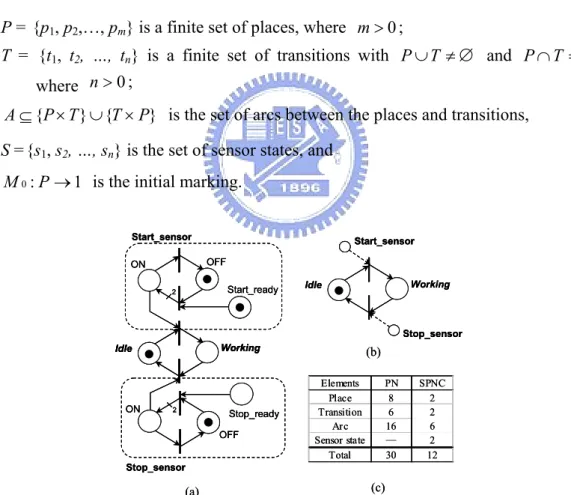
Fig. 3.1 (a) shows an ordinary PN model for pushing a button to trigger a process. By using the ordinary PN approach in controlling manufacturing processes, to deal with multiple sensor readings makes the net structure become more complicated and difficult to analyze. Therefore, by introducing the sensor state into the PN to form an SPNC, the
net structure becomes more simplified for implementation. From the control point of view, as shown in Fig. 3.1 (b), the sensor state in the SPNC replaces the reading sensor model such as push buttons or limit switches within the ordinary PN. Note that the condition of sensor states may change depending on the practical situation. Thus, as sensors increase in processes, the net structure of the SPNC is greatly simplified, as shown in Fig. 3.1 (c). Then, it becomes easy to model and implement the sequence controller through the SPNC defined as:
) , , , , ( SPNC= P T A S M0 (3.1) where,
P = {p1, p2,…, pm} is a finite set of places, where m>0;
T = {t1, t2, …, tn} is a finite set of transitions with P∪T ≠∅ and P∩T =∅,
where n>0; } { }
{P T T P
A⊆ × ∪ × is the set of arcs between the places and transitions,
S ={s1, s2, …, sn} is the set of sensor states, and
1 :
0 P→
M is the initial marking.
(a) Start_ready OFF ON 2 2 Working Idle OFF ON Stop_ready Start_sensor Stop_sensor Start_sensor Working Idle Stop_sensor (b) (c) Elements PN SPNC Place 8 2 Transition 6 2 Arc 16 6 Sensor state ― 2 Total 30 12 (a) Start_ready OFF ON 2 2 Working Idle OFF ON Stop_ready Start_sensor Stop_sensor Start_ready OFF ON 2 2 Working Idle Working Idle OFF ON Stop_ready Start_sensor Stop_sensor Start_sensor Working Idle Stop_sensor Start_sensor Working Idle Stop_sensor (b) (c) Elements PN SPNC Place 8 2 Transition 6 2 Arc 16 6 Sensor state ― 2 Total 30 12
Fig. 3.1. The comparison between the PN and the SPNC via a simple process. (a) Ordinary PN. (b) SPNC. (c) Comparison results.
3.1.2 Graphical Representation
As shown in Fig. 3.2, the SPNC consists of three kinds of nodes: 1) the place, drawn as a circle, 2) the transition, drawn as a bar, and 3) the sensor state, drawn as a smaller circle with a hidden arrow. The arcs, represented by directed arrows, are either from a place to a transition or from a transition to a place. In modeling, the marking conditions of places represent the status of the system and the transitions represent events. A transition has a set of input and output places, which represent the pre-conditions and post-conditions of the event, respectively. A sensor state, associated with its transitions, represents the sensor readings as a firing condition which triggers a manufacturing sequence. The sensor state is a Boolean variable that can be 0 in which case the related transition is not fired, or 1 in which case the related transition is fired if it is enabled. The marking of the SPNC is represented by the number of tokens in each place, drawn as black dots. The presence of a token in a given place means that the associated condition is true or that the actions associated with this place are taken.
Place Transition Token Arc Sensor state
Fig. 3.2. The icon definition of the SPNC.
3.1.3 Dynamic Behavior
The dynamic behavior of a system is simulated by the distribution of tokens in places as the enable transitions fire. The flow of tokens in the SPNC is governed according to the following rules:
1) Enabling rule:
A transition is said to be enabled, if all its input places are marked. 2) Firing rule:
Furthermore, the enabled transition is fired if all its sensor states are true. When an enabled transition fires, it removes one token from all its input places and deposits one token into all its output places at the same time.
3.1.4 Comparison with Other Models
The behavior of the proposed SPNC is similar to the sequential function chart (SFC). However, since SFC is derived from PN with some modifications and simplifications, theoretical results of PN cannot be directly applied to SFC (Miyazawa et al., 1997). Since the present SPNC is an extension of the PN by introducing sensor states, SPNC allows formal analysis of various properties, such as the safety, liveness, and reversibility for the process (David and Alla, 1994). Moreover, SFC only offers the method for depicting sequences of control system without providing any mechanisms to perform the functional analysis. Note that in the present IDEF0/SPNC/TPL/LLD approach, by applying the IDEF0 for functional analysis and information flow design, the SPNC model can be transformed from the information flow diagram.
Furthermore, compared with other extended PN applications such as Interpreted PN (Moalla, 1985), Automation PN (Uzam and Jones, 1998), or Signal Interpreted PN (Frey, 2000), which use external events to model sensor readings, the present SPNC simply applies the sensor states to model the firing conditions. Also, the present IDEF0/SPNC/TPL/LLD approach obtains the PLC programs systematically, from the design specifications through the SPNC, and to the final LLD. Since the PN model is inherently concurrent, whereas the LLD is typically scan-based, the sequential specification must be determinate and deterministic in the present approach. Also, the mono-marked restrictions design is required in the proposed SPNC to guarantee the safety of the sequence in practice.
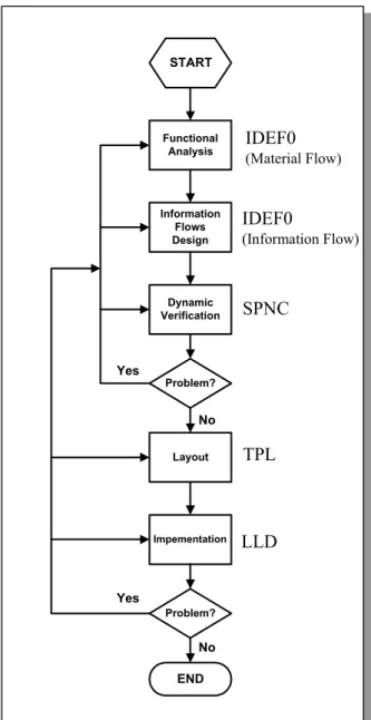
SPNC, and TPL tools, is proposed to systematically obtain the LLD for PLC implementation. The design procedure of the IDEF0/SPNC/TPL/LLD approach, depicted in Fig. 3.3, consist of five stages and each stage is described as follows.
Functional Analysis Information Flows Design END START Dynamic Verification Layout Impementation Problem? Yes No Problem? Yes No IDEF0 (Material Flow) IDEF0 (Information Flow) SPNC TPL LLD
3.2.1 Functional Analysis Stage: IDEF0
With the given specifications, the purpose of functional analysis is to realize the functions and operations of the system and then generate the control signals for the next stage. At this stage, each function of the manufacturing system has to be specified with a top-down hierarchically decomposing process by using the IDEF0 (Prabhaka, 1993). IDEF0 is an activity-oriented modeling approach and its representation of a manufacturing process consists of an ordered set of boxes representing activities performed by the system. The inputs are those items transformed by the activity and the outputs are the results of the activity, as shown in Fig. 3.4. The mechanisms, drawn as supporting arrows, represent resources such as machines, computers and operators, etc. The decomposition process continues until there is sufficient in detail on the basic activities to serve the purpose of sequence control. A functional model of the material flow diagram is obtained at this stage.
Activity Input Material/ Information flows Control Output Mechanism Material/ Information flows
Machines/ Computers/ Operators Parameters/ Rules
Fig. 3.4. The IDEF0 scheme.
3.2.2 Information Flow Design Stage: IDEF0
At this second stage, the information flow is used to control the material flow in a manufacturing system. The information flow diagram is constructed from the material flow diagram with static analysis, again using the IDEF0. In the information flow