Satellite Sensor Image Classification Using Cascaded
Architecture of Neural Fuzzy Network
Chin-Teng Lin, Yin-Cheung Lee, and Her-Chang Pu
Abstract—Satellite sensor images usually contain many
com-plex factors and mixed pixels, so a high classification accuracy is not easy to attain. Especially, for a nonhomogeneous region, gray values of satellite sensor images vary greatly and thus, direct statistic gray values fail to do the categorization task correctly. The goal of this paper is to develop a cascaded architecture of neural fuzzy networks with feature mapping (CNFM) to help the clustering of satellite sensor images. In the CNFM, a Kohonen’s self-organizing feature map (SOFM) is used as a preprocessing layer for the reduction of feature domain, which combines orig-inal multi-spectral gray values, structural measurements from co-occurrence matrices, and spectrum features from wavelet decomposition. In addition to the benefit of dimensional reduction of feature space, Kohonen’s SOFM can remove some noisy areas and prevent the following training process from being overor-iented to the training patterns. The condensed measurements are then forwarded into a neural fuzzy network, which performs supervised learning for pattern classification. The proposed cascaded approach is an appropriate technique for handling the classification problem in areas that exhibit large spatial variation and interclass heterogeneity (e.g., urban-rural infringing areas). The CNFM is a general and useful structure that can give us favorable results in terms of classification accuracy and learning speed. Experimental results indicate that our structure can retain high accuracy of classification (90% in average), while the training time is substantially reduced if our system is compared to the commonly used backpropagation network. The CNFM appears to be more reasonable and practical than the conventional implementation.
I. INTRODUCTION
S
ATELLITE sensor images for remote sensing usually con-tain large spatial variation and interclass heterogeneity, es-pecially in the applications of soils/cities distribution analysis (such as the urban-rural infringing areas) for the land devel-opment and the variation detection of clouds and volcano for weather forecasting and precaution. To tackle such sophisticated analysis and classification problems, it is important to combine different types of image features, including spectral and spa-tial data types and process these diverse features by an efficient data-fusion and classification scheme. The aim of this paper is to study various features of satellite sensor images and develop a nerual fuzzy network-based system that can assist us in ana-lyzing and classifying the information from satellite sensor im-ages automatically.Early investigations for satellite-sensor image classification have employed autocorrelation functions [1], power spectra,
rel-Manuscript received October 30, 1998; revised April 29, 1999.
The authors are with the Department of Electrical and Control En-gineering, National Chiao-Tung University, Hsinchu, Taiwan (e-mail: [email protected]).
Publisher Item Identifier S 0196-2892(00)02472-4.
ative frequencies of various gray levels on the unnormalized image [2], and the second-order gray level statistics method [3] to obtain texture features. These applications should be ex-tended to produce the classification with arbitrary patterns, not just targets of selected blocks with different textures. Others have applied Bayesian classifier [4] and Markov Random Field [5], [6] to obtain relative frequencies of individual and neighbors among a pixel. These structures are hard to obtain the required results when samples are insufficient. Moreover, the consump-tion of time to do the classificaconsump-tion should also be one of the considerations. Some researchers use neural networks [7]–[9] to produce the classification. The results show that the neural network is a feasible application to satellite sensor image clas-sification. However, since the satellite sensor images usually contain many complex factors and mixed pixels, a high clas-sification accuracy is not easy to attain. Especially for a nonho-mogeneous region, the gray values of its satellite sensor image vary greatly and thus, the direct statistic gray values fail to do the categorization task correctly. To handle complicated satellite sensor image classification problems accurately and efficiently, we first combine three types of features including original gray values, statistically structural measurements, and spectrum fea-tures as the inputs of a classification system. In this system, we develop a new cascaded architecture of neural fuzzy network with feature mapping (CNFM) to help the clustering of satellite sensor images. In the proposed classifier architecture, CNFM, the dimension of input feature space is first reduced by a neural network, and then these condensed measurements are forwarded into a neural fuzzy network for classification. The adoption of the neural network and fuzzy logic techniques in this work is based on the fact that the former is nonparametric and able to handle diverse data, and the latter is good at processing uncer-tain data and partially known information. Also, they are both fast in the classification process after being well trained.
In the proposed CNFM, the dimension of feature space is first reduced by the Kohonen’s self-organizing feature map (SOFM). No matter how many features and how many channels we used, each group of features in high dimension can be transformed into two-dimensional (2-D) coordinates by the 2-D Kohonen’s SOFM. Aside from the benefit of reduction in input dimension, SOFM can remove some noisy areas and can avoid the following training process being overoriented to the training patterns. After the inputs have been condensed by Kohonen’s SOFM, further classification will be performed by a neural fuzzy network (called SONFIN [12]). This cascaded architecture, named CNFM, is a general and effective structure that can give us favorable results in terms of classification accuracy and learning speed. Experimental result shows that 0196–2892/00$10.00 © 2000 IEEE
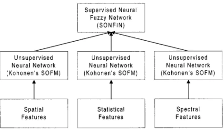
Fig. 1. Functional block diagram of the proposed CNFM.
the CNFM can reach the accuracy of 96.5% with respect to all domains of features based on the testing satellite sensor images that we had.
Fig. 1 shows the system architecture of CNFM. There are three types of inputs (features) that are spatial features of gray values, statistical features from a co-occurrence matrix, and spectral features from wavelet decomposition with channels. Suppose there are features in total. If we do not reduce our dimension of feature space, our network will need
input nodes. In the proposed CNFM, the input dimension is first reduced by the Kohonen’s SOFM and further classification is performed by a neural fuzzy network (SONFIN). In the next section, the acquirement, implementation, and modification of the three groups of features are given. In Section III, the integration of CNFM by cascading the Kohonen’s SOFM and SONFIN is modeled. Experimental results are shown in Section IV. Finally, some conclusions are made in Section V.
II. INPUTACQUISITION
The objective of this section is to clarify how the input tures are chosen and what they are actually for. These input fea-tures are gray values, statistical feafea-tures, and spectral feafea-tures. The varieties of different gray values among channels are char-acteristics that can be used to classify the ground cover types from data of multispectral spaces into desired clusters. How-ever, due to the complexities, mixed pixels, and diverse types of textures, we can make use of statistical features from a co-occur-rence matrix and spectral features from wavelet decomposition to improve the accuracy of classification.
A. Features from Spatial Domain by Multispectral Data Taking the advantage of multispectral data obtained from dif-ferent satellite sensors, we can classify the data as required. Here, we choose the gray values as our spatial features. Since the varieties of different gray values among channels can be served as characteristics, they can be used to classify the ground cover types in these multispectral spaces into desired clusters. In de-tails, the groups or clusters of pixel points are referred to as in-formation classes, since they are the actual classes of data that a computer can recognize.
B. Features from Statistical Domain
1) Co-occurrence matrix: Texture is a major distinguishing characteristic for the analysis of many types of images. On ac-count of the multispectral properties in satellite sensor image, texture also becomes an important characteristic for feature ex-traction. The gray-level co-occurrence matrices, proposed by Haralick et al. in 1973, constitute one of the basic approaches to the statistical analysis of texture [3] [14]. By computing a set of graytone spatial-dependence probability-distribution ma-trices for a given image block and extracting a set of textural features from each of these matrices, the basic model attempts to take the variation as a function of direction of spatial dis-tance [13]–[15]. We shall also develop some structural-statis-tical generalizations that apply the statisstructural-statis-tical techniques to ob-tain the structural features of satellite sensor images.
Consider the second-order histogram , where
, are gray values of pixels at distance apart and is the angle (usually every 45 ) of the line joining the centers of these
pixels. These matrices are symmetric (i.e.,
. From this matrix, a number of fea-tures can be computed. With gray levels in the image, the dimension of the matrix will be . The th element of this matrix is defined by [3]
(1)
where is the frequency of occurrence of gray levels and
separated by a distance and direction , , , .
The summation is over the total number of pixel pairs given , in the window.
We shall compute the following texture features from the co-occurrence matrix: angular second moment (ASM), contrast (CON), inverse difference moment (IDM), and entropy (ENT). These features are among the most commonly used co-occur-rence features [3], [13]–[15].
2) Simplification of Computations by Symmetric Linked-List (SLL): Since the number of operations required to compute any of the aforementioned features is proportional to the number of resolution cells (gray values being used) in the image block, co-occurrence matrices are time-consuming to compute and are memory-intensive as well. For a typical gray-valued image, as-suming that window size is and number of gray levels is (as usual, we set , and then the redundancy computation
is a factor of . To overcome this problem,
we use the full 256 (8 bits) dynamic range without compression and rely on efficiencies in our algorithm to overcome the com-putational demands of such large (256 256) matrices. This is in contrast to Haralick’s work in [14], where the number of gray levels was compressed to a more limited dynamic range. To take advantage of the characteristics of overlapped windows and symmetric property, we can construct a symmetric linked-list (SLL) [16], which is better suited for generating co-occurrence features than a matrix approach. Another advantage for using a gray-level co-occurrence linked list is efficiency, because it does not allocate storage for those gray-level pairs that have zero
TABLE I
ORDER OFCOMPLEXITY IN THE FIRST
COMPUTATION OFCO-OCCURRENCEMATRIX
TABLE II
ORDER OFCOMPLEXITYAFTER THEFIRSTCOMPUTATION OF
CO-OCCURRENCEMATRIX
probability. Each node in SLL consists of data , data , and a counter. Data and are indexes of the co-occurrence matrix, and the counter is used to count the frequency of occurrence of gray levels and . To increase the efficiency, each entry in SLL should be sorted. Since the co-occurrence matrix is symmetric, memory store can be reduced at least half.
The update procedure is as follows [13]–[16]. First, we con-struct a basic co-occurrence matrix at the left-top corner of the image and compute the required features from this matrix. Then, we subtract elements from the last column. Second, we move the window one column to the right. At the same time, we add elements from the new inserted column and compute the re-quired features. Repeat this process column by column. When the window reaches the end of the row, we slide down to the next row. Then, the window will move in a zigzag pattern until the entire image has been covered. Although it is not easy to design the SLL, it is the fastest method to calculate the co-occurrence matrix with full color range. Moreover, this update method can be usefully applied to other applications.
3) Order of Complexity: To calculate the order of com-plexity, we define N to be the size of neighborhood, G to be the number of gray levels, L1 to be the length of asymmetric linked-list, and L2 to be the length of symmetric linked-list. Since we use the full 256 (8 bits) dynamic range without compression in this work, the length of symmetric linked-list L2 is almost half (i.e., the nonredundant portion) of the length of asymmetric linked-list L1. Also, we define Co to be Co-occurrence matrix, Asym to be co-occurrence matrix with Asymmetric linked-list, and Sym to be co-occurrence matrix with Symmetric linked-list. Since the co-occurrence matrix is updated to calculate the order of complexity of subtraction and addition between rows (Horizontal), between columns (Vertical), and between slant of rows and of columns, we define H to be Horizontal, V to be Vertical, L to be slant toward Left, and R to be slant toward Right.
Tables I and II show the order of complexity of the first it-eration and each of the following itit-erations, respectively. Since there is no other consideration in overlapping area in Co, the
complexity of Table II is the same as that in Table I. However, for the linked-list format, the factor of is reduced to either L1 or L2, and the factor of is reduced to either 4 or 2, correspondingly. This is because we only need to update ei-ther two columns or two rows for the linked-list format. Furei-ther- Further-more, Since the length of L2 is almost half of the length of L1, the Symmetric format has the lowest computational complexity. 4) Global Texture Features from Second-Order Histogram Statistics: From the co-occurrence matrix, we can define the texture features as follows [3].
a) Entropy (ENT): The entropy computed from the second order histogram provides a standard measurement of homogeneity and is defined as
Entropy (2)
when stands for the total levels of gray value (i.e., in our
experiment, we set ). Higher values of
homo-geneity measures will indicate less structural variations, while lower values will be interpreted as a higher probability of tex-tural region.
b) Contrast (CON): The contrast feature is a difference moment of the matrix and is a standard measurement of the amount of local variations presented in an image. The contrast feature on the second-order histogram is defined as
Contrast (3)
The higher the values of the contrast are, the sharper the struc-tural variations in the image are.
c) Angular Second Moment (ASM): The angular second moment gives a strong measurement of uniformity and can be defined as
Angular Second Moment (4)
Higher nonuniformity values provide evidence of higher struc-tural variations.
d) Inverse Difference Moment (IDM): The inverse differ-ence moment is a measure of local homogeneity, and is defined as
Inverse Di erence Moment
(5) It is noticed that features such as correlation cannot be used, since if the variance becomes zero, the correlation will come to infinity.
C. Features from Spectrum Domain
The wavelet decomposition [10], [11] is a mathematical framework for constructing an orthonormal basis for the space of all finite energy signals. It can decompose input signals into multiscale details, describing their power at each scale and po-sition, so it can discriminate the local properties corresponding to smooth and textured areas. The framework of wavelet decomposition is based on the notion of a multiresolution analysis, which consists of a chain of approximation vector
spaces . In other words, just as sin and cos functions are orthogonal, so the set of scaled and dilated wavelets forms an orthonormal basis for [10], [11]. The first basis consists of a set of scaling functions [10]
(6) where is a scaling factor that forms an orthonormal basis for . Besides, there is a corresponding set of functions, a wavelet basis [10],
(7) that forms an orthonormal basis for . The spaces , are mutually orthogonal.
In practice, the approximation and detailed projection coef-ficients associated with and are computed from the ap-proximation coefficients at the next higher scale using a quadrature mirror filter pair (QMF) and a pyramidal sub-band coding scheme. The impulse responses of the QMF pair are
typ-ically denoted by and , where is formed from the
inner product between and , and is formed
from the inner product between and , i.e.,
and (8)
(9) The coefficients have to meet several conditions for the set of basis functions to be unique and orthonormal. It can be shown that a wavelet decomposition of a signal does not re-quire the explicit forms of and , but only depends on and sequences. Moreover, filtering operations use and coefficients as the impulse responses corsponding to low and high-pass operations, respectively. By re-peatedly convoluting each approximation signal with and , and decimating the outputs by a factor of two, the signal is decomposed into frequency bands whose bandwidths and center frequencies vary by octaves.
In this paper, we choose the quadratic spline function as the scaling function [11], i.e.,
(10)
The Fourier transform of its corresponding wavelet is
(11)
Then we can deduce the coefficients and as
fol-lows [11], [17]:
(12)
(13)
Fig. 2. Procedure of wavelet decomposition.
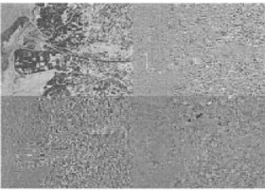
Fig. 3. Result of wavelet decomposition of a channel input, where the top left and bottom right are the result of wavelet decomposition from both low pass and from both high pass in columns and in rows, respectively. The top right image is from low pass in columns and high pass in rows. Conversely, the bottom left image is from high pass in columns and low pass in rows.
where can be selected as [17]
and for
The complete procedure is shown in Fig. 2. First, we select a point from the left-top of the image and obtain a block from the gray values of its neighbors. Second, we perform the wavelet de-composition row by row, including cases of low pass and high pass. Finally, we apply the same process column by column. This is the 2-D wavelet decomposition [17]. For the wavelet de-composition, we first extend the size of the selected block to be a square block. Then, we perform the convolution and down-sample the size of the block into half. Afterwards, we transpose the image for the next wavelet decomposition. As an illustrated example shown in Fig. 3, the left-top and right-bottom images are the result of wavelet decomposition from both low pass, and from both high pass in columns and in rows, respectively. The right-top image is from low pass in columns and high pass in rows. Conversely, the left-bottom image is from high pass in columns and low pass in rows.
III. CASCADEDARCHITECTURE OFNEURALFUZZYNETWORK WITHFEATUREMAPPING(CNFM)
After we have obtained the features from the spatial, statis-tical, and spectral domains, we proceed with the training of
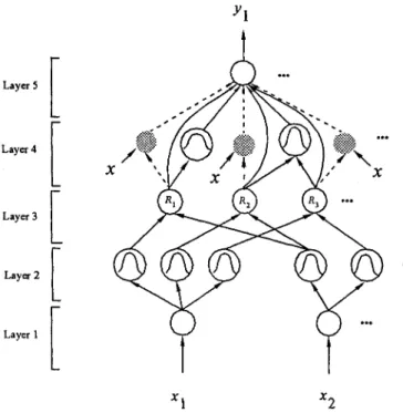
clas-Fig. 4. Structure of Self-Constructing Neural Fuzzy Inference Network (SONFIN).
sification by our system, CNFM. It is composed of two cascaded neural networks. The former one is the unsupervised Kohonen’s SOFM and the latter is the supervised neural fuzzy network (called SONFIN). From Fig. 4, we can see the detailed infor-mation of the architecture. For each channel, we obtain thirteen types of features as the inputs of Kohonen’s SOFM and get the individual outputs, where the output of each SOFM is the 2-D coordinates (on the x and y axes) in the map formed by the 2-D neurons (clustering units). In this way, we transform the thirteen statistic measurements into three 2-D coordinates for each channel. Next, we use the supervised neural fuzzy network, SONFIN, to produce a refined classification. This complemen-tary architecture can compensate the problems of inaccuracy and long training time of unsupervised and supervised neural networks, respectively. It is noticed that although the concept of cascading a supervised neural network by an unsupervised learning neural network is not an entirely new concept in the neural network realm for speeding up learning, the proposed ar-chitecture is a totally new combination. In addition to owning the advantage of speedy learning, more importantly, the pro-posed architecture provides a new efficient solution to the pat-tern recognition problems containing many diverse types of fea-tures, thus making a contribution to the domain of pattern recog-nition in general and remote sensing classification in particular. In more details, the most important contribution of this archi-tecture is to improve the method of input selection. Compared to the conventional trial and error approach, the input dimen-sion of our system is first reduced by the Kohonen’s SOFM, and then each group of features from a channel is transformed into 2-D coordinates. Consequently, with benefit of input dimension reduction, Kohonen’s SOFM unsupervised neural network also contributes to noise elimination. Next, we use SONFIN to over-come the inaccuracy due to Kohonen’s SOFM. Hence, no matter
how many features and how many channels that we use, the problem of big input space and long training time can be re-moved by the proposed mechanism.
A. Reduction of Input Dimension by Unsupervised Network This subsection introduces the 2-D Kohonen’s SOFM, which can map high-dimensional inputs onto a 2-D map and can filter out some noisy information [19]. In addition to mapping high-dimensional inputs onto a 2-D map, another major goal of Kohonen’s SOFM is to obtain a topology-preserving map that keeps the neighborhood relations of the input patterns. We shall also modify the Kohonen’s SOFM to make the input clusters be normally distributed. With the benefits of Kohonen’s SOFM, the system can be adapted to the change of increase of both features and channels easily. Also, it can filter out some noisy information. The most important merit is that we can avoid taking trial and error to remove redundancy, such as by genetic algorithm, KL expansion, and correlation
.
The 2-D SOFM, also called a topology-preserving map, as-sumes a topological structure among the cluster units. There are cluster units, arranged in a 2-D array in our application, the input signals are tuples. The weight vector for a cluster unit serves as an exemplar of the input patterns associated with that cluster. During the self-organization process, the cluster unit whose weight vector matches the input pattern most closely (typically, the square of the minimum Euclidean distance) is chosen as the winner. The winning unit and its neighboring units (in terms of the topology of the cluster units) update their weights. The 2-D coordinates (on the and axes) of the win-ning unit on the 2-D map of SOFM are viewed as the output of SOFM.
To make an unsupervised neural network utilize the informa-tion concerning the distribuinforma-tion of patterns, the patterns must be divided into clusters according to the occurrences of clus-ters. Therefore, clusters will be sufficient enough in a high-den-sity region, whereas the number of clusters will be reduced in a sparse region. We apply this conscience [18] into the update of the Kohonen’s SOFM. After the selection of a winner, i.e.,
if
otherwise,
(14)
where is the winner, is the current inputs, is the weight vector (cluster ), and instead of updating the weights as usual, we record the usage of each cluster, i.e.,
(15) where is the record of usage and is a step size. After the statistics are known, the selection of the winner will be rewritten as
if
otherwise,
(16)
where is an offset, and is a constant.
As the usage of cluster increases, its offset will de-crease. This reduces its competitive ability. In other words, its
conscience is increased and is persuaded to give opportunity to other clusters.
B. Classification by Supervised Network
After the transformation of input space using Kohonen’s SOFM has been completed, we then pass the newly composed inputs into a supervised neural network to produce a refined classification. This cascaded architecture has the ability to perform the classification of satellite sensor images even though there are very complex mixed pixels.
The neural fuzzy network that we used for satellite sensor image classification is called the self-constructing neural fuzzy inference network (SONFIN) that we proposed previously in [12]. It is worth mentioning that SONFIN is a brand new idea applied to satellite sensor image classification. The SONFIN is a general connectionist model of a fuzzy logic system, which can find its optimal structure and parameters automatically. The number of generated rules and membership functions is small even for modeling a sophisticated system. The SONFIN can always find itself an economic network size, and the learning speed as well as the modeling ability are all appreciated as com-pared to normal neural networks.
The structure of SONFIN is shown in Fig. 4. The five-layered network realizes a fuzzy model of the following form
Rule IF is and and is
THEN is
where is a fuzzy set, is the center of a symmetric mem-bership function on , and is a consequent parameter. It is noted that unlike the traditional TSK model [19], where all the input variables are used in the output linear equation, only the significant ones are used in the SONFIN (i.e., some ’s in the above fuzzy rules are zero). We shall next describe the functions of the nodes in each of the five layers of the SONFIN.
Layer 1: This layer is an input layer
(17) Layer 2: Each node in this layer corresponds to one lin-guistic label (small, large, etc.) of one of the input variables in Layer 1. With the use of the Gaussian membership function, the operations performed in this layer are
(18) where and are, respectively, the center (or mean) and the width (or variance) of the Gaussian membership function of the th term of the th input variable .
Layer 3: A node in this layer represents one fuzzy logic rule and performs precondition matching of a rule. Here, we use the following AND operation for each Layer-3 node
(19)
where is the number of Layer-2 nodes participating in the IF part of the rule.
Layer 4: This layer is called the consequent layer. Two types of nodes are used in this layer, and they are denoted as blank and shaded circles in Fig. 4, respectively. The node denoted by a blank circle (blank node) is the essential node representing a fuzzy set (described by a Gaussian membership function) of the output variable. The function of the blank node is
(20)
where the center of a Gaussian membership function. As to the shaded node, it is generated only when necessary. The shaded node function is
(21)
where the summation is over all the inputs, and is the cor-responding parameter. Combining these two types of nodes in Layer 4, we obtain the whole function performed by this layer for each rule as
(22)
Layer 5: Each node in this layer corresponds to one output variable. The node integrates all the actions recommended by Layers 3 and 4 and acts as a defuzzifier with
(23)
The SONFIN can be used for normal operation at any time during the learning process without repeated training on the input-output patterns when online operation is required. There are no rules (i.e., no nodes in the network except the input/output nodes) in the SONFIN initially. They are created dynamically as learning proceeds upon receiving online incoming training data by performing the following learning processes simultaneously:
1) input/output space partitioning; 2) construction of fuzzy rules; 3) consequent structure identification; 4) parameter identification.
Processes 1, 2, and 3 belong to the structure learning phase, and process 4 belongs to the parameter learning phase. The details of these learning processes can be found in [12].
C. Cascaded Architecture of Neural Fuzzy Network with Feature Mapping (CNFM)
This subsection gives the details of how to implement the cas-caded architecture of the unsupervised and supervised neural networks presented in Section III-A and III-B, respectively. The general architecture of CNFM is set up as follows. At first, we utilize (e.g., ), Kohonen’s SOFM’s to reduce the di-mensions of sets of inputs. The full (three) sets of inputs that we have here are gray values, statistical properties, and spec-trum features from wavelet decomposition. Instead of using all
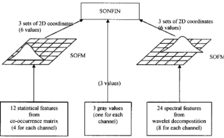
Fig. 5. System architecture of the CNFM used in our experiment.
sets of selected features as the inputs of a supervised neural net-work, the Kohonen’s SOFM can transform each set of features into 2-D coordinates and use these low-dimension data as the inputs of the supervised neural fuzzy network, SONFIN. Not only can we get a better representation, but we can also obtain a good meaning when the 2-D coordinates serve as the inputs of a supervised neural network.
To go into a little more detail, Fig. 5 shows the architecture of our system. The first set of inputs contains three gray values, each of which comes from one of three channels and repre-sents the features of spatial domain. The second set of inputs consists of angular second-moment, contrast, inverse difference moment, and entropy that come from co-occurrence matrices. This set of inputs represents the features of statistical domain. The last set of inputs includes energy and entropy that come from wavelet decomposition and represents the features of spec-tral domain. After the transformation of Kohonen’s SOFM’s, these three sets of inputs are reduced into 2-D coordinates. How-ever, we do not expand a gray value into 2-D coordinates be-cause its dimension is low enough in our test examples. Also, if we have transformed the gray values of all channels, we may re-move the information of differences among channels. Since the statistical and spectral features focus on local varieties, we can apply the transformation directly and do not need to care for the information of differences among channels. As a result, we re-duce the input dimension from 39 features (13 features/channel 3 channels) into 15 features (5 features/channel 3 chan-nels, where each channel has one gray value and two 2-D co-ordinates). As shown in Fig. 5, the three types of inputs are a gray value obtained from each channel, four statistical fea-tures from each channel, and eight spectral feafea-tures from each channel, where there are three channels totally. Hence, if we have not reduced our dimension of inputs, there are 39 inputs in total. It must be noted that if the number of features increase, the number of inputs will grow terribly.
After the feature domain has been reduced and transformed by the Kohonen’s SOFM, we pass the condensed measurements to a supervised neural fuzzy network SONFIN. This network can perform online input space partitioning, which creates only the significant membership functions on the universe of dis-course of each input variable by using a fuzzy measure algo-rithm [12] and the orthogonal least square (OLS) method [19]. Our objective is to use SONFIN to obtain lower mean square
error (MSE) and higher learning rate. The result will be com-pared to that of normally used statistics and backpropagation-network schemes in Section IV.
IV. EXPERIMENTALRESULTS
Our experiment makes use of the real High Resolution Vis-ible (SPOT HRV) satellite sensor images provided by the Earth Resource Satellite Receiving Station in R.O.C. The image size of each channel is 1024 1024, with full 256 gray levels. These images contain five classes, with respect to soil (Class 1), forest (Class 2), sea (Class 3), city 1—residential area (Class 4) and city 2—industrial area (Class 5). These five classes are defined entirely based on the ground truth obtained by onsite investi-gation. Due to the different properties of these five classes, we believe their morphologies also differ, giving them different tex-tures. We find that some of these classes are expected to be highly separable from each other (i.e., soil, forest, and sea), but the others (i.e., city 1 and city 2) are quite similar since both of them are urban, although city 1 is the residential area and city 2 is the industrial area. The requirement of distinguishing city 1 from city 2 makes this classification problem more difficult. Our experiment will demonstrate this phenomena and show the need for combining diverse types of features in the proposed CNFM. Our objective is to classify these classes from the three-channel satellite sensor images. The results show that when we try to use all features as inputs directly without any dimension reduction to perform the training of classification on either a SONFIN or a backpropagation (BP) network, the converged MSE is so large that we cannot reduce it. Hence, we must first apply the SOFM in our CNFM to reduce the dimension of inputs and then per-form the training of classification.
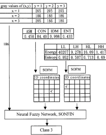
An illustrative example for classification of the features from a channel using CNFM is shown in Fig. 6, and it can give the de-tails of the proposed system. First, we obtain the gray value of a center-pixel, 186. From the neighborhood of this pixel, we then calculate the Angular Second Moment (ASM), Contrast (CON), Inverse Difference Moment (IDM), entropies and energies from the co-occurrence matrices and wavelet transformations with a neighborhood size . After we have acquired the input features, we pass each group of the features into a Kohonen’s SOFM. Then, each group of input features with high dimension is reduced to 2-D coordinates. Finally, we use these 2-D coor-dinates, combined with the coordinates from other channels, as the inputs of the neural fuzzy network SONFIN. The result we obtained is the desired cluster, and its name is Class 3. In our ex-periments, the learning parameters of SOFM, including neigh-borhood size, learning rate, and convergent rate are set as fol-lows:
1) neighborhood size: initial value is 100 and updated by (i.e., the shrinkage term)
neighborhood size epoch
2) learning rate: initial value is 0.9 and updated by
Fig. 6. Illustrative example for classification of the features from a channel using CNFM.
TABLE III
CLASSIFICATIONRESULT WITHALLTYPES OFFEATURES
3) convergent rate: convergent rate is updated by
number of training set total number of training set
In SONFIN, the learning rate , overlap degree
, similarity degree , forgetting factor
, threshold parameters , and are
chosen. After 50 000 time steps of training, 18 input clusters (rules) are generated. The final converged MSE is 12.74.
Tables III–V show the results of the classification using the proposed CNFM. Here we compared the classification accu-racies resulting from different types of inputs. Based on the satellite sensor images that we had, the result in Table III got the average classification accuracy of 96.5% and was the best among the others, because all information was used as inputs to CNFM in this case. Table IV shows the result of classifi-cation using only the information of gray levels and statistics
TABLE IV
CLASSIFICATIONRESULT WITHGRAYVALUES ANDSTATISTICSFEATURES
TABLE V
CLASSIFICATIONRESULT WITHGRAYVALUESONLY
and therefore, the average classification accuracy decreased to 94.9%. We can see that the classification accuracy decreased in each class. The last one is Table V, and the result was obtained with three gray values only. The average classification rate be-came 92.5%. Table V tells us that the gray levels alone are only good at distinguishing Class 3 (sea) from the others. By com-paring Tables IV and V, we find that the statistics features do en-hance the discriminative power of gray levels on Class 1 (soil) and Class 2 (forest), but not on Class 4 (city 1—residential area) and Class 5 (city 2—industrial area). By comparing Tables III and IV, we find that the spectrum features can further enhance the discrimination power of gray levels and statistics features on the two urban areas, Class 1 and Class 2. It can thus be seen that without sufficient information, classification is difficult to perform. Fig. 7 shows the ground truth of the satellite sensor image and the classified image using CNFM with three types of features. We see that CNFM can perform quite an accurate classification.
Table VI shows the classification results of the nearest-neighborhood (KNN) method [19], BP network [19], and the CNFM. The inputs of BP network and CNFM are first filtered by Kohonen’s SOFM, whereas KNN uses all features directly. In other words, the compared BP network is actually in the same structure as the CNFM, but the SONFIN in CNFM is replaced by a normal BP network. We had also tried to use the normal BP network by feeding all the 39 features (13 features for each channel) into it directly as inputs without going through Ko-honen’s SOFM for the reduction of feature space. However, the learning of this BP network appeared very slow, and the MSE was keeping at quite a high value. That is, it was stuck at a very bad local minimum, since the network was too big. Hence, we do not present the experimental results of this BP network here. The BP network used has two hidden layers with 30 hidden nodes in each layer, trained by the standard backpropagation learning rule with momentum term, where the learning rate was
Fig. 7. Ground truth of the satellite sensor image used in the experiment (top) and the classified result of CNFM (bottom), where industrial area, soil, sea, forest, residential area are all denoted, the areas enclosed by squares are training patterns, and the other areas are testing patterns.
TABLE VI
COMPARISON OF THECLASSIFICATIONRESULTSAMONGKNN, BP,ANDCNFM
set as 0.5, the momentum parameter was set as 0.9, and the training time was 2300 epochs (about 50 000 time steps). The network structure, as well as the learning constants, were de-termined after thorough trial-and-error testing for achieving the best performance (i.e., lowest MSE). The learning was stopped when the MSE almost kept constant. Table VI shows that the CNFM outperforms the KNN and BP network in average
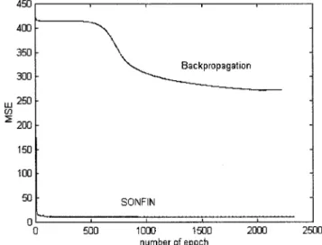
Fig. 8 shows the accuracy and MSE of BP network against SONFIN in our CNFM. We can conclude that the BP network is insufficient to reduce the MSE due to the complexity of the image sources, but our system can tackle this problem success-fully. From Tables III–VI of our experiments, we can summa-rize that not only the proposed diverse types of features, but also the cascaded model, CNFM, can enhance the classification ac-curacy of satellite sensor images of the traditional approaches. However, although the experiment based on our satellite sensor image shows that the accuracy improvement is somewhat signif-icant, the exact extent to which the classification accuracy can be increased by the proposed scheme depends on the particular satellite sensor images tested.
V. CONCLUSIONS
The major contribution of the proposed system is to pro-vide a good solution to the problem of scaling and selection of satellite sensor image features. Hence, in this paper, we provide some auxiliary information to handle problems of diverse types of textures and the varieties of neighborhood in the sophisti-cated satellite sensor image classification problems. However, the additional features will increase the computation complexity a great deal and mislead the training. To overcome this problem, we present a new cascaded system (called CNFM) that uses Kohonen’s self-organizing feature map as the reduction mecha-nism of input dimension. After we have obtained the condensed measurements, a fine classification on them is performed by a neural fuzzy network (called SONFIN).
The major contribution of the proposed system is to solve the problem of scaling and selection of image features well. Also, we extended the mechanism of Kohonen’s SOFM in the sense of reducing the high input dimension rather than filtering the training sets. Our CNFM, combining spatial, statistical, and spectral features into one system, generalizes well and can avoid the network parameters orienting to the training patterns. Furthermore, we improved the computation complexity of the co-occurrence matrix by the symmetric linked-list structure. Our future work is to enhance our cascaded system by using edge information. Edge information can be used as an outline of the distribution of clusters and to improve the classification accuracy.
REFERENCES
[1] H. Kaizer, “A quantification of textures on aerial photographs,” Boston Univ. Res. Lab., Boston University, Boston, MA, Technical note 121, AD 69484, 1955.
[2] E. M. Darling and R. D. Joseph, “Pattern recognition from satellite al-titudes,” IEEE Trans. Syst. Sci. Cybern., vol. SSC-4, pp. 38–47, Mar. 1968.
[3] R. M. Haralick, K. Shanmugam, and I. Dinstein, “Texture features for image classification,” IEEE Trans. Syst., Man, Cybern., vol. SMC-3, pp. 610–621, 1973.
[4] J. M. Boucher, P. Lena, and J. F. Marchand, “Application of local and global unsupervised Bayesian classification algorithms to the forest,”
IGARSS ’93, Better Understanding of Earth Environment (Cat. No. 93C3294-6), vol. 2, pp. 737–739, Aug. 1993.
[5] E. Rignot and R. Chellappa, “Segmentation of polarimetric synthetic aperture radar data,” IEEE Trans. Image Processing, vol. 1, pp. 281–299, July 1992.
[6] A. H. S. Solberg, T. Taxt, and A. K. Jain, “A Markov random field model for classification of multisource satellite imagery,” IEEE Trans. Geosci.
Remote Sensing, vol. 34, pp. 100–113, Jan. 1996.
[7] Y. Hara, G. Atkins, S. . Yueh, R. T. Shin, and J. A. Kong, “Application of neural networks to radar image classification,” IEEE Trans. Geosci.
Remote Sensing, vol. 32, pp. 100–109, Jan. 1994.
[8] Y. C. Tzeng, K. S. Chen, W. L. Kao, and A. K. Fung, “A dynamic learning neural network for remote sensing applications,” IEEE Trans.
Geosci. Remote Sensing, vol. 32, pp. 994–1102, Sept. 1994.
[9] Y. C. Tzeng and K. S. Chen, “AS fuzzy neurasl network to SAR image classification,” IEEE Trans. Geosci. Remote Sensing, vol. 36, pp. 301–307, Jan. 1998.
[10] I. Daubechies, “Orthonormal bases of compactly supported wavelets,”
Commun. Pure Appl. Math., vol. 41, pp. 909–996, Nov. 1988.
[11] S. G. Mallat, “Multiresolution approximation and wavelets orthonormal base of L (R),” Trans. Amer. Math. Soc. 1989, vol. 315, pp. 69–88, Sept. 1989.
[12] C. F. Juang and C. T. Lin, “An on-line self-constructing neural fuzzy inference network and its applications,” IEEE Trans. Fuzzy Syst., vol. 6, pp. 12–32, Feb. 1998.
[13] P. Gong, D. J. Marceau, and P. J. Howarth, “A comparison of spatial feature extraction algorithms for land-use classification with SPOT HRV data,” Remote Sens. Environ., vol. 40, pp. 137–151, May 1992. [14] R. M. Haralick, “Statistical and structural approaches to texture,” in
Proc. IEEE, vol. 67, May 1979, pp. 786–804.
[15] D. R. Peddle and S. E. Franklin, “Image texture processing and data in-tegration for surface pattern discrimination,” Photogramm. Eng. Remote
Sensing, vol. 57, no. 4, pp. 413–420, 1991.
[16] D. Clausi and M. Jernigan, “A fast method to determine co-occurrence texture features,” IEEE Trans. Geosci. Remote Sensing, vol. 36, no. 1, pp. 298–300, 1998.
[17] J. W. Hsieh, M. T. Ko, H. Y. Liao, and K. C. Fan, “A new wavelet-based edge detector via constrained optimization,” Image Vis. Comp., vol. 15, pp. 511–527, July 1997.
[18] D. DeSieno, “Adding a conscience to competitive learning,” in Proc.
IEEE ICNN, vol. 1, San Diego, July 1988, pp. 117–124.
[19] C. T. Lin and C. S. G. Lee, Neural Fuzzy Systems: A Neural-Fuzzy
Syn-ergism to Intelligent Systems (with disk). Englewood Cliffs, NJ: Pren-tice-Hall, 1996.
[20] P. L. Palmer and M. Petrou, “Locating boundaries of textured regions,”
IEEE Trans. Geosci. Remote Sensing, vol. 35, pp. 1367–1371, Sept.
1997.
Chin-Teng Lin received the B.S. degree in control engineering from the National Chiao-Tung Univer-sity (NCTU), Hsinchu, Taiwan, R.O.C., in 1986, and the M.S.E.E. and Ph.D. degrees in electrical engi-neering from Purdue University, West Lafayette, IN, in 1989 and 1992, respectively.
Since August 1992, he has been with the College of Electrical Engineering and Computer Science, NCTU, where he is currently a Professor of Elec-trical and Control Engineering. He has also served as the Deputy Dean of the Research and Development Office of NCTU since 1998. His current research interests are fuzzy systems, neural networks, intelligent control, human-machine interface, and video and audio processing. He is the co-author of Neural Fuzzy Systems—A Neuro-Fuzzy
Synergism to Intelligent Systems and the author of Neural Fuzzy Control Systems with Structure and Parameter Learning. He has published around 40
journal papers in the areas of neural networks and fuzzy systems.
Dr. Lin is a member of Tau Beta Pi and Eta Kappa Nu. He is also a member of the IEEE Computer Society, the IEEE Robotics and Automation Society, and the IEEE Systems, Man, and Cybernetics Society. He has been an Execu-tive Council Member of Chinese Fuzzy System Association (CFSA) since 1995 and the Supervisor of Chinese Automation Association since 1998. He was the Vice Chairman of IEEE Robotics and Automation, Taipei Chapter, in 1996 and 1997. He won the Outstanding Research Award granted by National Science Council (NSC), Taiwan, in 1997 and 1999, and the Outstanding Electrical En-gineering Professor Award granted by the Chinese Institute of Electrical Engi-neering (CIEE) in 1997.
Yin-Cheung Lee received the B.S. and M.S. degrees in electrical and control engineering from the National Chiao-Tung University, Hsinchu, Taiwan, R.O.C., in 1996 and 1998, respectively.
His current research interests include pattern recognition, neural networks, remote sensing, and image analysis. He is currently a System Researcher with Formosoft Software Inc., Taiwan.
Her-Chang Pu received the M.S. degree in automatic control engineering from Feng-Chia University, Taichung, Taiwan, R.O.C., in 1998. He is pursuing his Ph.D. degree in electrical and control engineering at National Chiao-Tung University, Hsinchu, Taiwan.
His current research interests are in the areas of ar-tificial neural networks, fuzzy systems, pattern recog-nition, and machine vision.